 Oleg Gaidai1
 Yihan Xing
 Shuaishuai Wang
- 1Shanghai Engineering Research Centre of Marine Renewable Energy, College of Engineering Science and Technology, Shanghai Ocean University, Shanghai, China
- 2Department of Mechanical and Structural Engineering and Materials Science, University of Stavanger, Stavanger, Norway
- 3Norwegian University of Science and Technology, Trondheim, Norway
Extreme value prediction of the load-effect responses of complex offshore structures such as the floating wind turbine (FWT) is crucial in ultimate limit state (ULS) design. This paper considers two cases to understand the feasibility of the bivariate correction on the extreme load and motion responses of a 10-MW semi-submersible type FWT. The empirical anchor tension force and surge motion used in this study are obtained from the FAST simulation tool (developed by the National Renewable Energy Laboratory) with the load cases stimulated at under-rated, rated and above rated speeds. Then, the bivariate correction method is applied to model FWT extreme response for a 5-years return period prediction with a 95% confidence interval (CI), based on just 2 min short response record. The proposed methodology permits accurate correction of the bivariate extreme value in case of, for example, corrupted measurement sensor data. Based on the proposed novel method’s performance, it is concluded that the bivariate correction method can offer better robust and precise bivariate predictions of coupled surge motion and anchor tension of the FWT.
1 Introduction
The environmental pollution caused by the massive use of fossil fuels has triggered the transformation of non-renewable energy to renewable energy. In 2020, global energy-related carbon dioxide emissions dropped by 5.8%, which reached the highest record of the percentage decrease since the second World War. Meanwhile, renewable energy reached 29%, the highest record share in global electricity (Secretariat, 2021). As one of the most promising renewable energy, wind energy has been evolving rapidly. 93 GW of new wind power installations was seen in 2020, which brought the global cumulative wind power capacity up to 743 GW (Council, 2021).
Although today’s wind generation is mainly onshore, a great prospect is predicted for floating offshore wind. This is because floating wind turbines (FWTs) could harvest vast wind resources over deep water, where the wind capacity is more than four times the bottom-fixed wind. However, the high cost is the main challenge with the floating wind turbines. This is mainly due to the small scale of the floating wind farms and the immaturity of the technology and supply chain. Significant technology improvement is a must to overcome the challenges and lower the levelized cost of energy (LCOE) of floating wind. Enhancing the insights into the loads and load effects of the FWTs will be an efficient solution to the successful deployment of floating wind. This is because a good understanding of the FWT dynamics can aid to reduce the risk and uncertainty associated with the wind turbine design and operating, thus reducing the turbine, foundation and operating expenses.
Mooring equipment is a crucial cost driver within the floating wind, while significant efforts need to be taken to develop a target safety level to realise a cost-effective design of mooring systems. Ultimate limit state (ULS) check serves as the main criteria for the mooring system design, which is performed based on extreme load effect analysis. The FWT is a complex combination with aerodynamics, hydrodynamics, control system and flexible structures and is subjected to various environmental conditions with wind, wave and currents. Determining the extreme values of the mooring system requires effective methods to deal with the extreme analysis problem.
Hsu et al. (Hsu et al., 2015) presented a comparative analysis in predicting the extreme mooring line tensions of an FWT exposed to a 100-years storm condition between model test and numerical simulations. The importance of the snap events to the mooring line tensions was investigated based on the exceedance probability analysis, and results showed that normalised snap loads tend to a constant 3, which can contribute to determining the safety factor of mooring lines. In the study of Hsu et al. (Hsu et al., 2017), a composite Weibull probability distribution was proposed for the mooring line dynamic tensions due to the effects of snap loads. The results showed that when the probability of the snap events is high, the developed composite Weibull distribution method could be effectively used to predict extreme tensions of FWT mooring systems. Xu et al. (Xu et al., 2019a) studied the influence of non-linear wave kinematics on fatigue damage and extreme responses of a 5MW semi-submersible FWT. Gumbel fitting and Average Conditional Exceedance Rate (ACER) methods were used to predict the extreme values of linear mooring tensions, and the results showed that the fully non-linear wave theory would lead to higher mooring line tensions than the linear wave theory. Cao et al. (Cao et al., 2020) investigated the extreme responses of a new concept of 10-MW semi-submersible FWT based on the experimental tests. The mean up-crossing rate method was used to estimate the extreme short-term values of the mooring linear tensions. The results showed that the extreme mooring line tensions are more likely to occur under harsh environmental conditions than operational conditions. Most of the previous studies predicting the extreme loads of mooring line tensions are based on the extreme value distribution models.
However, the extreme values predicted by this method depend on the tail of the probability distributions, which are pretty sensitive to uncertainties. The well developed ACER method can enhance the effectiveness and reliability in predicting the extreme values, but significant numerical or experimental efforts are needed to produce sufficient data for the ACER analysis. Motivated by this, it is essential to improve the method to predict extreme responses without devoting significant costs and efforts accurately.
This paper proposes a novel bivariate correction approach if the sensor malfunctions or the available data record is too short. The proposed method can more efficiently and reliably predict extreme loads in a 10 MW large floating wind turbine (FWT). More efficient and reliable estimations of extreme responses will better help predict the effects these loads have on the components allowing the development and implementation of a better design or control system for the FWT. Optimal wind turbine parameters would minimise potential FWT mechanical damage due to excessive environmental loadings (Xu et al., 2019a). Accurately predicted extreme loads will also allow the components to be more optimally sized. It contributes to more refined designs and lower failure rates, which is particularly important for the offshore wind industry as it advances the design, manufacturing and deployment of large FWTs (>10 MW) in the coming decade.
2 System Description
A 10-MW FWT system (Yu et al., 2017) is used in this work, and is illustrated in Figure 1. The FWT system will be expounded in two parts in the following sections. Firstly, the reference wind turbine will be described, then the properties of the semi-submersible floater and the mooring system will be introduced Figures 2 and 3.
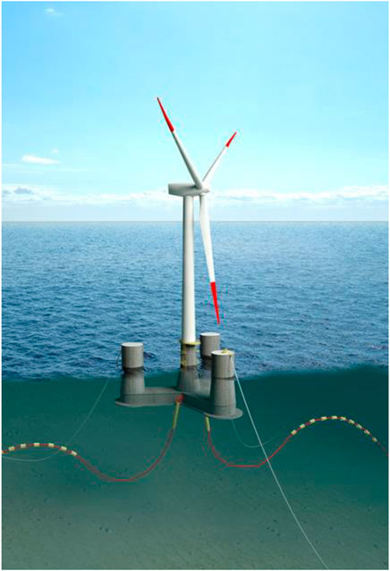
FIGURE 1. The 10-MW OO-Star floating wind turbine (Yu et al., 2017).
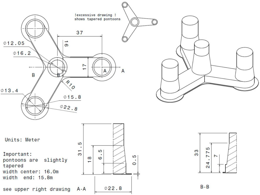
FIGURE 2. Main dimensions of the OO-Star floater of the 10-MW wind turbine.
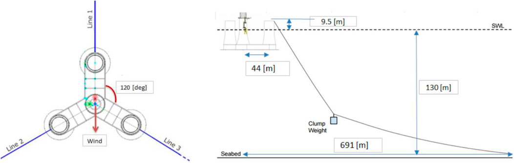
FIGURE 3. Sketch of the mooring system in the 10-MW FWT (left: top view; right: side view).
2.1 DTU 10-MW Reference Wind Turbine
The DTU 10-MW reference wind turbine (RWT) is used in this paper, designed from the NREL 5-MW RWT. The wind turbine was designed per the International Electrotechnical Commission (IEC) Class 1A wind regime and is a traditional three-bladed, clockwise rotation-upwind turbine equipping with a variable speed and collective pitch control system. The DTU 10-MW RWT numerical model has been successfully developed and studied in many academic works, e.g., (Hu et al., 2021; Muggiasca et al., 2021; Wang et al., 2022; Yu et al., 2022). The summary of the DTU 10-MW RWT is shown in Table 1.

TABLE 1. Key parameters of the DTU 10-MW reference wind turbine (Yu et al., 2017).
2.2 OO-Star Semi-Submersible Wind Floater and Mooring System
This work uses a semi-submersible floating structure to support the 10-MW RWT. It was introduced by Dr. techn. Olav Olsen AS in the LIFES 50 + project (Yu et al., 2017). The floater comprises post-tensioned concrete, hosting a central column with three outer columns. The four columns are mounted on a star-shaped pontoon, where a slab is attached at the bottom. Three catenary mooring lines are used to maintain the floater in position, and in each line, a clumped mass is attached, separating the line into two segments. Greater details of the OO-Star Wind Floater and the mooring system are shown in Table 2 and Table 3, respectively.
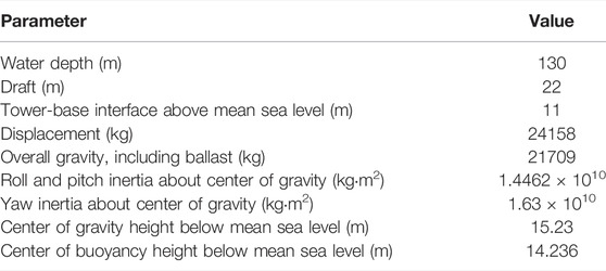
TABLE 2. The main properties for the 10-MW OO-Star wind floater.
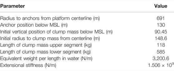
TABLE 3. The main properties for the mooring system of the 10-MW FWT.
3 Methodology
This section describes the methodology adopted by authors to address engineering challenges related to safe and reliable design of FWTs (floating wind turbines). Note that the proposed ACER (Average Conditional Exceedance Rate) method along with The FAST simulation tool was already recently successfully used by the authors, see, e.g., (Xu et al., 2020).
3.1z Aero-Hydro-Elastic-Servo Dynamic Analysis of the 10-MW FWT
FAST (Fatigue, Aerodynamics, Structures and Turbulence) (version8, v8.16.00a-bjj), an open-source WT simulation tool developed by the National Renewable Energy Laboratory (NREL), is utilised in this work for the fully coupled aero-hydro-elastic-servo dynamic analysis for the 10-MW FWT. The FAST code couples together five computer codes: AeroDyn (Moriarty and Hansen, 2005), HydroDyn (Jonkman et al., 2014), ServoDyn, and MoorDyn (Hall, 2015), to account for the aerodynamic loads on rotor blades, hydrodynamic loads on floaters, control dynamics, structural dynamics and mooring system dynamics. In addition, FAST provides the interface for reading the time-varying stochastic wind for time-domain simulations. The FAST simulation tool has been successfully used in other well-known projects such as OC3: Offshore Code Comparison Collaboration (Jonkman and Musial, 2010) and OC4: IEA Task Wind 30 (Robertson et al., 2014), and its modelling capability has been authenticated using multiple floating structures in the Netherlands (Coulling et al., 2013).
3.1.1 Aerodynamics
The blades aerodynamic loads are calculated based on the quasi-steady Blade Element Momentum (BEM) theory. BEM theory combines momentum theory and blade element theory. Various advanced corrections, including tip loss, hub loss, skewed inflow and dynamic stall corrections, are included in the BEM method. The Prandtl corrections are implemented to account for the hub and blade tip losses due to a finite number of blades. The Glauert correction is applied to account for the induction factors, while the Pitt and Peters' model accounts for the skewed inflow correction. The dynamic stall correction is employed in the Beddoes-Leishman model. More details about the aerodynamic load calculation in the FAST code can be seen in the AeroDyn theory manual (Moriarty and Hansen, 2005).
3.1.2 Hydrodynamics
Hydrodynamic loads acting on the semi-submersible floater are calculated based on potential flow theory with Morison’s drag term considered. It accounts for the wave pressures and viscous loads, respectively. Hydrodynamic coefficients, such as added mass and potential damping coefficients, and first-order wave excitation load transfer function are firstly estimated in the frequency domain by a panel code, WAMIT, according to the potential flow theory. These hydrodynamic coefficients are then transformed into the time domain using the convolution technique.
3.1.3 Structural Dynamics
A combined multi-body and modal structural approach is considered in the FAST code to account for the structural dynamics of the FWT. The blades, tower and driveshaft are considered flexible bodies, while the nacelle, hub and floater are rigid bodies. The inherent structural damping in the blades and tower are represented using the Rayleigh damping model. The structural dynamic responses in the time-domain are calculated by solving the equations of motion of the rigid-flexible coupled system derived by Kane’s approach, see (Kane and Levinson, 1983).
3.1.4 Control System Dynamics
The control system used in the 10-MW FWT is implemented in two operational modes: the below-rated and full-rated regions. The generator torque-speed curve regulates the rotor rotational speed with an optimal tip speed ratio in the below-rated region, achieving maximum power generation. A proportional-integral (PI) algorithm regulates the blade pitch angle to reduce the structural loading while keeping the rated power generation in the full-rated region. The PI parameters are modified from the land-based RWT to avoid the negative damping effects, which are essential in affecting the platform motions for FWTs.
3.2 ACER Method
Consider a long term global response process (such as anchor tension force or FWT surge motion) X (t) of the FWT, measured over a time interval
and
Where
The measured time series can be subdivided into K subsequent (short term) blocks such that
Where
In the above equations, an assumption of ergodicity has been used for each short term segment of the recorded time series in order to estimate the short term expected values by using observed values of the
Where
Where
As the order k increases, the accuracy of Eqn. 7 improves and
The
It is suggested to do the optimisation on the log-level by minimising the following mean square error function F with respect to the four arguments
Where
3.3 Bivariate Correction
As already mentioned, the method proposed in this paper will be based on the ACER methodology. This involves both the univariate ACER functions and the bivariate ACER functions. The unique feature of the ACER functions is that they provide the possibility to portray the exact extreme value distribution inherent in the data time series, both the univariate and the bivariate (Wang, 2001)- (Xu et al., 2019b). Hence, the ACER method is fundamentally different from the traditional approach relying on the fitting of hardly asymptotic data to asymptotic extreme value distributions, which are based on the assumption of stationary time series instead of the ACER method. The empirical ACER functions are represented in nonparametric numerical functions with uncertainty bounds. The accuracy obtained depends, of course, on the amount of data available to estimate these functions. It is also an essential feature of the ACER method that it is not limited to stationary time series. It is entirely valid for nonstationary time series as long as the measured data reflects this nonstationarity. For the sake of easy reference, the univariate ACER methodology has been briefly outlined below. The bivariate case follows quite closely the univariate case.
This section presents a statistical bivariate integral correction based on the bivariate ACER method coupled with the Gumbel logistic model (Gaidai et al., 2019a)- (Xu et al., 2019b). Note that this correction is not limited to only extreme value estimates. However, it can be applied with appropriate bivariate models for any statistical values of interest to improve their accuracy based on synchronously measured longer, highly correlated data records.
Let
Raw response time series with
with
In this model, it is seen that m = 1 corresponds to the case when
The numerical estimates
Note that all quantities on the right side of Eqn. 12 are known from the available time series of recorded data. The Gumbel copula parameter
4 Bivariate Correction Results
Three realistic mean wind velocities of 8, 12 and 16 m/s are studied in this paper. For the three environmental conditions, 20 different random samples of wind and wave are applied for each sea state. Each simulation lasts 4000s, where the first 400s is removed to reduce the transient effect induced by the wind turbine start-up. Therefore, 1-h data in each simulation is formed and is used for extreme value analysis in this work. The results shown in this work are based on the average of 20 1-h simulations to reduce the stochastic variability.
Simulated surge motion and anchor tension,
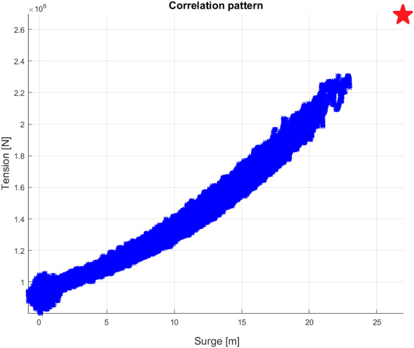
FIGURE 4. Phase space between simulated
Figure 5 shows the ACER functions for the more extended observation period
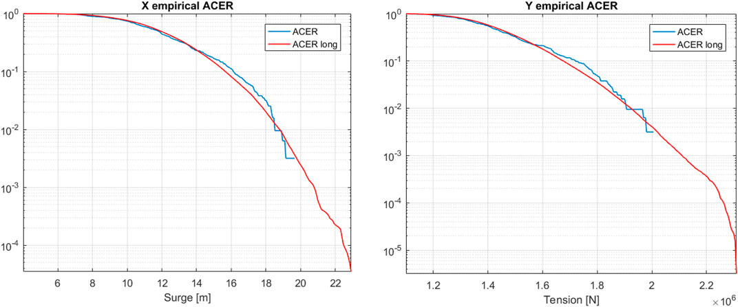
FIGURE 5. ACER functions for shorter and longer FWT response records:
The following results were obtained for the simulated FWT response motions bivariate correction.
Table 4 presents the correction results for the corrected FWT anchor

TABLE 4. Correction results for measured FWT response: 20 h (long) and 2 min (short). Five years return period prediction.
5 Conclusion
The FWT surge motion and anchor tension force due to environmental wind and wave loads were studied for three operating conditions of mean wind speeds of 8, 12 and 16 m/s. The bivariate correction method was briefly described and applied to account for the coupled load effects, namely surge motion and anchor tension force simulated synchronously in time.
This paper proposed using the bivariate correction method to investigate the extreme structural responses (motion surge and anchor tension force) during FWT realistic operation. High correlation between the two processes is the key requirement for the described correction to achieve improved prediction accuracy. As shown in the presented study, there is a practical advantage in applying the bivariate correction introduced in this paper, as it brings prediction based on short time series of data quite close to the prediction based on a much longer time series. Thus, a significant improvement in extreme value prediction accuracy is obtained. Some practical situations that may justify the above-mentioned analysis would be:
⁃ Another similar FWT is being designed for the same environmental condition, then data collected from one FWT may be useful for another.
⁃ Malfunctioning of one measuring sensor, while another is well-functioning.
This paper shows that applying the bivariate correction for the particular cases studied has increased extreme FWT response prediction accuracy. This improvement shows that the proposed correction method can be useful in engineering design in case of sensor malfunctioning or available data record is too short.
Data Availability Statement
The raw data supporting the conclusions of this article will be made available by the authors, without undue reservation.
Author Contributions
OG, Writing, Conceptualisation, Method, Analysis, Discussion. YX, Writing, Conceptualisation, Method, Analysis. FW, Funding, Review, Discussions. SW, Analysis, Writing. PY, Discussions. AN, Review, Discussions.
Conflict of Interest
The authors declare that the research was conducted in the absence of any commercial or financial relationships that could be construed as a potential conflict of interest.
Publisher’s Note
All claims expressed in this article are solely those of the authors and do not necessarily represent those of their affiliated organizations, or those of the publisher, the editors and the reviewers. Any product that may be evaluated in this article, or claim that may be made by its manufacturer, is not guaranteed or endorsed by the publisher.
References
Bak, C., Zahle, F., Bitsche, R., Kim, T., Yde, A., Henriksen, L. C., and Natarajan, A. (2013). “The DTU 10-MW Reference Wind Turbine,” in Danish Wind Power Research 2013.
Cao, Q., Xiao, L., Cheng, Z., Liu, M., and Wen, B. (2020). Operational and Extreme Responses of a New Concept of 10MW Semi-submersible Wind Turbine in Intermediate Water Depth: An Experimental Study. Ocean. Eng. 217, 108003. doi:10.1016/j.oceaneng.2020.108003
Coulling, A. J., Goupee, A. J., Robertson, A. N., Jonkman, J. M., and Dagher, H. J. (2013). Validation of a FAST Semi-submersible Floating Wind Turbine Numerical Model with DeepCwind Test Data. J. Renew. Sustain. Energy 5 (2), 023116. doi:10.1063/1.4796197
Council, G. W. E. (2021). GWEC| Global Wind Report 2021. Brussels, Belgium: Global Wind Energy Council.
Gaidai, O., Naess, A., Karpa, O., Xu, X., Cheng, Y., and Ye, R. (2019). Improving Extreme Wind Speed Prediction for North Sea Offshore Oil and Gas Fields. Appl. Ocean Res. 88, 63–70. doi:10.1016/j.apor.2019.04.024
Gaidai, O., Naess, A., Xu, X., and Cheng, Y. (2019). Improving Extreme Wind Speed Prediction Based on a Short Data Sample, Using a Highly Correlated Long Data Sample. J. Wind Eng. Industrial Aerodynamics 188, 102–109. doi:10.1016/j.jweia.2019.02.021
Gaidai, O., Storhaug, G., and Naess, A. (2016). Extreme Large Cargo Ship Panel Stresses by Bivariate ACER Method. Ocean. Eng. 123, 432–439. doi:10.1016/j.oceaneng.2016.06.048
Gaidai, O., Xu, X., Wang, J., Ye, R., Cheng, Y., and Karpa, O. (2020). SEM-REV Offshore Energy Site Wind-Wave Bivariate Statistics by Hindcast. Renew. Energy 156, 689–695. doi:10.1016/j.renene.2020.04.113
Hall, M. (2015). MoorDyn User’s Guide, 15. Orono, ME, USA: Department of Mechanical Engineering, University of Maine.
Hsu, W.-t., Thiagarajan, K. P., and Manuel, L. (2017). Extreme Mooring Tensions Due to Snap Loads on a Floating Offshore Wind Turbine System. Mar. Struct. 55, 182–199. doi:10.1016/j.marstruc.2017.05.005
Hsu, W. T., Thiagarajan, K. P., MacNicoll, M., and Akers, R. (2015).Prediction of Extreme Tensions in Mooring Lines of a Floating Offshore Wind Turbine in a 100-year Storm, Int. Conf. Offshore Mech. Arct. Eng., 56574. V009T09A050. doi:10.1115/omae2015-42015
Hu, R., Le, C., Gao, Z., Ding, H., and Zhang, P. (2021). Implementation and Evaluation of Control Strategies Based on an Open Controller for a 10 MW Floating Wind Turbine. Renew. Energy 179, 1751–1766. doi:10.1016/j.renene.2021.07.117
Jian, Z., Gaidai, O., and Gao, J. (2018). Bivariate Extreme Value Statistics of Offshore Jacket Support Stresses in Bohai Bay. J. Offshore Mech. Arct. Eng. 140 (4). doi:10.1115/1.4039564
Jonkman, J. M., Robertson, A. N., and Hayman, G. J. (2014). HydroDyn User's Guide and Theory Manual. Golden, CO: National Renewable Energy Laboratory.
Jonkman, J., and Musial, W. (2010). Offshore Code Comparison Collaboration (OC3) for IEA Wind Task 23 Offshore Wind Technology and Deployment (No. NREL/TP-5000-48191). Golden, CO (United States): National Renewable Energy Lab NREL.
Kane, T. R., and Levinson, D. A. (1983). The Use of Kane's Dynamical Equations in Robotics. Int. J. Robotics Res. 2 (3), 3–21. doi:10.1177/027836498300200301
Moriarty, P. J., and Hansen, A. C. (2005). AeroDyn Theory Manual (No. NREL/TP-500-36881). Golden, CO (US): National Renewable Energy Lab.
Muggiasca, S., Taruffi, F., Fontanella, A., Di Carlo, S., Giberti, H., Facchinetti, A., et al. (2021). Design of an Aeroelastic Physical Model of the DTU 10MW Wind Turbine for a Floating Offshore Multipurpose Platform Prototype. Ocean. Eng. 239, 109837. doi:10.1016/j.oceaneng.2021.109837
Naess, A., and Karpa, O. (2015). Statistics of Bivariate Extreme Wind Speeds by the ACER Method. J. Wind Eng. Industrial Aerodynamics 139, 82–88. doi:10.1016/j.jweia.2015.01.011
Naess, A., and Karpa, O. (2015). Statistics of Extreme Wind Speeds and Wave Heights by the Bivariate ACER Method. J. Offshore Mech. Arct. Eng. 137 (2). doi:10.1115/1.4029370
Robertson, A., Jonkman, J., Musial, W., Popko, W., and Vorpahl, F. (2014). IEA Wind Task 30 Offshore Code Comparison Collaboration Continued.
Wang, Q. J. (2001). A Bayesian Joint Probability Approach for Flood Record Augmentation. Water Resour. Res. 37 (6), 1707–1712. doi:10.1029/2000wr900401
Wang, S., Moan, T., and Jiang, Z. (2022). Influence of Variability and Uncertainty of Wind and Waves on Fatigue Damage of a Floating Wind Turbine Drivetrain. Renew. Energy 181, 870–897. doi:10.1016/j.renene.2021.09.090
Xu, K., Zhang, M., Shao, Y., Gao, Z., and Moan, T. (2019). Effect of Wave Nonlinearity on Fatigue Damage and Extreme Responses of a Semi-submersible Floating Wind Turbine. Appl. Ocean Res. 91, 101879. doi:10.1016/j.apor.2019.101879
Xu, X.-s., Gaidai, O., Karpa, O., Wang, J.-l., Ye, R.-c., and Cheng, Y. (2021). Wind Farm Support Vessel Extreme Roll Assessment while Docking in the Bohai Sea. China Ocean. Eng. 35 (2), 308–316. doi:10.1007/s13344-021-0028-x
Xu, X., Gaidai, O., Naess, A., and Sahoo, P. (2020). Extreme Loads Analysis of a Site-specific Semi-submersible Type Wind Turbine. Ships Offshore Struct. 15 (Suppl. 1), S46–S54. doi:10.1080/17445302.2020.1733315
Xu, X., Gaidai, O., Naess, A., and Sahoo, P. (2019). Improving the Prediction of Extreme FPSO Hawser Tension, Using Another Highly Correlated Hawser Tension with a Longer Time Record. Appl. Ocean Res. 88, 89–98. doi:10.1016/j.apor.2019.04.015
Yu, W., Müller, K., Lemmer, F., Bredmose, H., Borg, M., Sanchez, G., et al. (2017). Public Definition of the Two LIFES50+ 10MW Floater Concepts. LIFES50+ Deliv. 4.
Keywords: floating wind turbine, FAST, bivariate correction method, extreme responses, bivariate probability distribution
Citation: Gaidai O, Xing Y, Wang F, Wang S, Yan P and Naess A (2022) Improving Extreme Anchor Tension Prediction of a 10-MW Floating Semi-Submersible Type Wind Turbine, Using Highly Correlated Surge Motion Record. Front. Mech. Eng 8:888497. doi: 10.3389/fmech.2022.888497
Received: 02 March 2022; Accepted: 11 May 2022;
Published: 04 July 2022.
Edited by:
Shahrum Abdullah, Universiti Kebangsaan Malaysia, MalaysiaReviewed by:
Ping Liu, Jiangsu University of Science and Technology, ChinaJuchuan Dai, Hunan University of Science and Technology, China
Copyright © 2022 Gaidai, Xing, Wang, Wang, Yan and Naess. This is an open-access article distributed under the terms of the Creative Commons Attribution License (CC BY). The use, distribution or reproduction in other forums is permitted, provided the original author(s) and the copyright owner(s) are credited and that the original publication in this journal is cited, in accordance with accepted academic practice. No use, distribution or reproduction is permitted which does not comply with these terms.
*Correspondence: Yihan Xing, eWloYW4ueGluZ0B1aXMubm8=