 Vishwas Deep Joshi1
 Ajay Kumar
 Lenka Cepova
- 1Department of Mathematics, Faculty of Science, JECRC University, Jaipur, Rajasthan, India
- 2Department of Mechanical Engineering, School of Engineering and Technology, JECRC University, Jaipur, Rajasthan, India
- 3Department of Machining, Assembly and Engineering Metrology, Faculty of Mechanical Engineering, VSB-Technical University of Ostrava, Ostrava, Czechia
- 4Department Department of Mechanical Engineering, Faculty of Engineering and Technology, Jain (Deemed-to-be) University, Bengaluru, India
- 5Department of Mechanical Engineering, Vivekananda Global University, Jaipur, India
- 6Department of Orthodontics, Faculty of Dental Sciences, SGT University, Gurugram, Haryana, India
Amidst uncertainty, decision-making in manufacturing becomes a central focus due to its complexity. This study explores complex transportation constraints and uses novel ways to guide manufacturers. The Multi-objective Stochastic Linear Fractional Transportation Problem (MOSLFTP) is a crucial tool for managing supply chains, manufacturing operations, energy distribution, emergency routes, healthcare logistics, and other related areas. It adeptly addresses uncertainty, transforming efficiency and effectiveness in several domains. Stochastic programming is the process of converting theoretical probabilities into concrete certainties. The artistic compromise programming technique acts as a proficient mediator, reconciling opposing objectives and enabling equitable decision-making. This novel approach also addresses the Multi-objective Stochastic Linear plus Linear Fractional Transportation Problem (MOSLPLFTP), which involves two interconnected issues. The effectiveness of these principles is clearly shown with the help of the LINGO® 18 optimization solver. This study uses a ranking method to compare the similar methods to solve the current problems. A meticulously designed example acts as a significant achievement, shedding light on our method in a practical setting. It serves as a distinctive instrument, leading manufacturers through the maze of uncertainty and assisting them in determining the most advantageous course of action. This journey involves subtle interactions between complexity and simplicity, uncertainty is overcome by decisiveness, and invention is predominant.
1 Introduction
The transportation problem, a fundamental aspect of operations research, seeks to achieve efficiency. The main objective is to find the best cost-effective method for transporting items from several production units to many warehouses. This challenge requires lowering costs while meeting supply and demand requirements. It will assist the business in making optimum decisions and developing effective advertising strategies. Suppliers, customers, their capabilities, and transportation costs are often arranged in a matrix arrangement in a standard representation. The goal is to distribute product quantities from suppliers to customers efficiently by meeting needs, adhering to supply constraints, and reducing prices. Linear programming methods are often used to produce an optimum solution by determining how resources should be distributed throughout the network for the greatest results. The transportation problem originated in the mid-20th century when Koopmans (Koopmans, 1949) developed its formal formulation in 1947 to solve logistical problems, especially during World War II. This mathematical problem requires the optimal distribution of commodities from different suppliers to various demand locations in order to minimize transportation expenses. The development of the simplex approach (Dantzig, 1963) during the same era significantly boosted the optimization field by enhancing the efficiency of solving linear programming problems, such as the transportation problem. With the rise of computers in the 1960s and 1970s, the range of solutions to problems increased to handle intricate real-world situations. The problem’s applications evolved further, leading to the emergence of current algorithms such interior point approaches in the 1990s for improved efficiency in finding answers. Currently, in a time of complex supply chains, the transportation problem is still relevant, with sophisticated optimization software consistently expanding its uses in many sectors. Picture a large industrial complex looking to enhance the efficiency of its transportation network. Stochastic programming develops mathematical models to achieve stability, punctual delivery, and cost savings while considering operational constraints. Stochastic modelling and flexible optimization are used to manage unexpected elements like supply chain disruptions and demand variations, ensuring that the transportation plan can adapt to unanticipated events. Implementing this strategy enhances a manufacturing facility’s sustainability and competitive edge within its sector by tackling transportation problems and optimizing supply chain operations. This enhances resource distribution, environmental stewardship, and cost efficiency.
The linear fractional transportation problem involves managing resource allocation to reduce costs or enhance producer profits. It combines linear programming techniques, which optimize linear objective functions under linear constraints, with fractions. Resources may be subdivided into fractional units, which is very useful in situations such as delivering components of a product. The linear plus linear fractional transportation problem further complicates this complexity. This advanced version includes fractional elements and adds another level of complexity. This layer establishes linear linkages in both the goal function and restrictions. Picture it as a puzzle with two levels - optimizing fractions and managing linear connections—creating a more complex and engaging challenge for those solving problems.
Stochastic programming (SP) is a powerful tool for decision-making in manufacturing, especially in dealing with uncertainty. It combines mathematical optimization with probability theory to create solutions that navigate smoothly through the constantly changing and mysterious circumstances of reality. Imagine it as a navigator on rough seas, plotting a path that not only endures the storm but flourishes in it. SP’s canvas spans several fields, with transportation and industry being notable areas. In the transportation industry, it coordinates routes, manages fleets, and responds to emergencies, all while navigating through unpredictability. SP excels in the industrial environment by optimizing production processes, maintenance, energy distribution, and risk management. It guarantees consistent efficiency in directing decision-makers with knowledge, even in an uncertain environment. Imagine a corporation that specialized in creating and transporting perishable goods. Here, SP is the focal point, creating an exceptional plan for manufacturing and distribution tactics. It achieves this by carefully considering unpredictable factors such as changing demand and irregular supply. Stochastic programming reveals the best production levels and distribution routes by considering various situations such as increased demand during holidays or supply delays caused by unexpected transportation problems. The firm reduces expenses, increases earnings, and remains robust and prepared for the uncertain market. SP, the master of flexibility and anticipation orchestrates this symphony of achievement.
Utilizing a Weibull distribution optimization method in mathematical modelling helps producers achieve equilibrium among conflicting goals, such as reducing costs, minimizing lead times, and enhancing service quality. Implementing supply chains, using stochastic modelling to manage demand variations, and optimizing transportation routes are some of these strategies. Commence construction work. Construction is under progress. This includes the design. Seek practical uses, particularly in multi-objective optimization. Excellence in environmental sustainability and customer service. Manufacturers may address difficult supply chain and transportation difficulties efficiently by using this advanced technology. This ultimately improves customer satisfaction and operational efficiency by enabling them to be flexible and responsive in a constantly evolving production environment.
In this article, we explore uncertainty using probability theory, focusing on Stochastic Programming (SP). We are exploring stochastic programming challenges, which include the integration of probability and mathematical programming to illuminate decision-making processes influenced by random factors. We begin our voyage by investigating a Stochastic Transportation Problem, which is a complex maze with many linear fractional objective functions. The MOSLFTP model is shaped by the limitations provided by normal random variables, forming a complex mathematical structure. Our goal is to discover a collection of Pareto-optimal solutions by balancing opposing goals inside MOSLFTP, rather than achieving an exact approximation of the true Pareto front. Researchers have explored many approaches (Table 1) to solve complicated problems. Stochastic programming techniques are essential tools that provide assistance in dealing with optimization difficulties that include random parameters. They explore a broad range of situations where model coefficients are influenced by uncertainty and follow certain probability distributions. Stochastic Programming has a wide-reaching impact on several fields such as management science, engineering, and technology. In fields where input data is unpredictable and models are created from imperfect information, SP finds its refuge. In recent years, its potential has greatly expanded due to advancements in computer science and optimization methods. It establishes itself and thrives in the industrial sector, revolutionizing energy resource planning, finance, telecommunications, transportation, production scheduling, and supply chain management into successful environments. SP showcases the limitless adaptability of probabilistic exploration in decision-making.
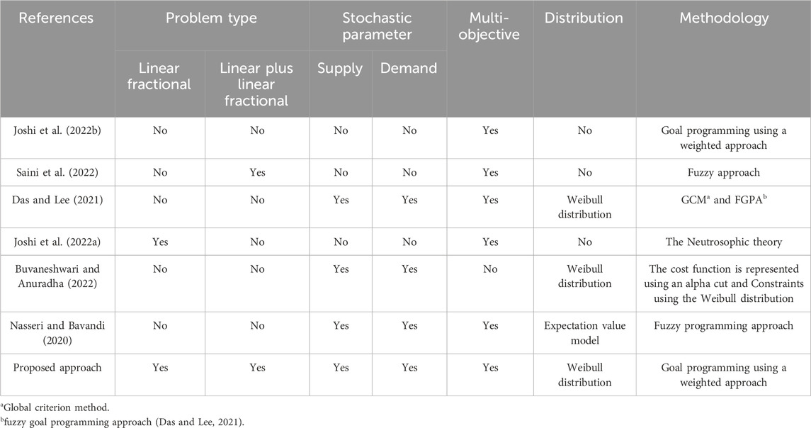
Table 1. These research efforts have played a vital role in deepening our grasp of the Transportation Problem, particularly in situations where uncertainty and complexity are at play.
The journey of the linear fractional transportation problem began with Swarup’s pioneering suggestion (Swarup, 1966), marking the genesis of this mathematical challenge. Since then, the literature (Sadia et al., 2016; Safi and Seyyed, 2017) has meticulously chronicled its systematic evolution, with scholars delving deeper into its intricacies. In the realm of solving transportation problems with fractional objectives, valuable methods were laid out by (Pradhan and Biswal, 2015), offering practical solutions for real-world scenarios where parameters may not always be precise, requiring a touch of educated guesswork. The murkiness of real-world problems, often obscured by a lack of specific data, led Liu (Liu, 2007) to unearth the uncertainty theory, reshaping our approach to these enigmas. Within this ever-expanding landscape, various scholars have turned to Stochastic Programming (SP) as a powerful tool for wrangling uncertainty. The SP model itself had its origins in the visionary work of Dantzig (Dantzig, 2011), and over time, it has blossomed into various incarnations with different scholars proposing their own SP models (Goicoechea and Duckstein, 1987). The intersection of stochasticity and fractional objectives has been a rich field of exploration, as evidenced by numerous investigations into the Stochastic Fractional Transportation Problem and its accompanying solution methodologies (Charles and Dutta, 2005; Jain and Arya, 2013; Jadhav and Doke, 2016). Javaid (Javaid et al., 2017) introduced a Transportation Problem model adorned with multiple fractional objectives and unpredictable parameters, adding layers of complexity to the puzzle. In the more recent annals of research, Saini’s work in 2022 (Saini et al., 2022) employed a fuzzy approach to untangle the knots of an MFL (Multi-Fractional Linear) paradox within a multi-objective transportation problem. Meanwhile, Joshi (Joshi et al., 2022a) embarked on an exploration of fractional transportation problems within the realm of neutrosophic situations in the same year, where all the objective function coefficients, demands, and availabilities existed in the realm of speculation. These contemporary inquiries highlight the ongoing pursuit of novel solutions to complex problems in the ever-evolving world of optimization and uncertainty management.
A technique for resolving MOSSTP in the presence of uncertainty by recasting it as a chance-constrained programming problem and employing fuzzy goal programming and the global criterion method to quickly find effective solutions (Das and Lee, 2021). A weighted goal programming method that, using a numerical example, discovers compromise solutions for multi-objective transportation problems following the decision-maker’s priorities (Joshi et al., 2022b). The Weibull distribution and multiple cost coefficients are used in a solution methodology for the multi-choice stochastic transportation problem (Roy, 2014). Using a Weibull distribution to describe the uncertain parameters, the research presents three models for dealing with stochastic fuzzy transportation problems (SFTPs) with mixed-type constraints (Buvaneshwari and Anuradha, 2022). Using a fuzzy technique, multiple-choice parameters, and random variables, a transportation problem with multiple objectives is solved (Nasseri and Bavandi, 2020).
The MOSLFTP is a complex mathematical conundrum that goes beyond the limits of a basic enigma. It explores the complex process of maximizing resource allocation from suppliers to consumers while managing several competing goals, similar to meeting various preferences at the same time. A mist of uncertainty overlays this intricacy, with specific numbers adhering to the elusive Weibull distribution pattern. Picture a complex labyrinth with several destinations, each with fluctuating circumstances. Your objective is to map out the most optimal route while managing competing objectives and moving through the haze of uncertainty. The MOSLFTP and MOSLPLFTP are intricately connected via the LINGO® 18.0 Software, which acts as a set of tools that work together to optimize processes. An example will demonstrate the effectiveness of this technique by leading us through ambiguity and helping us make well-informed judgments. This research serves as a crucial tool for companies seeking guidance in navigating complicated issues and uncovering the keys to success. Recent research has shed light on creative paths in manufacturing, urban transportation, and multi-objective optimization, paving the way for a more enlightened future (Kumar et al., 2020; Kumar and Gulati, 2021; Boadh et al., 2022; Kumar et al., 2022; Kumar et al., 2023a; Kumar et al., 2023b; Yadav et al., 2023).
This study is an innovative investigation into stochastic programming, focusing on a complex problem involving multiple linear and linear fractional objective functions. The problem incorporates supply and demand parameters that adhere to the Weibull distribution. The complex mathematical task is named MOSLPLFTP, representing a significant advancement in the subject. An extensive examination of current literature has shown a notable finding—there is a lack of study on these particular topics. This work is unique and innovative, exploring uncharted territory in research. This research also includes supply and demand variables that follow the Weibull distribution (Krishnamoorthy, 2006). By doing this, it creates a more complex and captivating specialization within the field of stochastic programming. This study is pioneering an examination of uncharted mathematical area, expanding the limits of knowledge, and creating opportunities for future investigations in optimization and uncertainty management.
A continuous probability distribution called the Weibull distribution can be used to model a variety of variables, such as the time to failure, the interval between events, and extreme values. It was first thoroughly described in 1939 by Swedish mathematician Waloddi Weibull, after whom it is called. The Weibull distribution has a wide range of applications, including Reliability engineering, Life data analysis, Engineering, Biology, Economics etc. The Weibull distribution’s probability density function with the known parameters
and
where
➢ Shape parameter
➢ Scale parameter
➢ Location parameter (
The remainder of this paper is thoughtfully organized into several sections, each playing a crucial role in advancing the understanding and exploration of the research topic. Basic definitions, notation and Weibull distribution-based mathematical models defined for MOSLFTP and MOSLPLFTP are discussed in Section 2. Then, the solution methodology is presented in Section 3. While Section 4 offers additional approaches. Numerical examples are discussed in the Section 5. The presentation of results and insightful discussions take center stage in Sections 6, with the ultimate conclusions elegantly summarized in Section 7. This organized structure guides readers through a comprehensive journey of discovery and insight in the realm of optimization and uncertainty management.
2 Methodology
2.1 Basic definitions
• Feasible solution: A feasible solution embodies the essence of a valid and practical resolution to a problem, one that harmoniously aligns with the stipulated conditions and constraints.
• Ideal solution: An ideal solution stands as the pinnacle of desirability, representing the most favourable and sought-after outcome among all feasible solutions. In the realm of multi-objective optimization, where multiple conflicting objectives for attention, there may exist multiple ideal solutions that collectively form a Pareto front.
• Anti-ideal solution: The anti-ideal solution, in stark contrast to the ideal solution, is distinguished by its unfavourable characteristics. It represents the solution with the poorest values for the objectives or embodies the most extreme violations of constraints within the problem space.
• Optimal solution: An optimal solution stands as the epitome of achievement, representing the result that attains the best conceivable outcome in alignment with the defined criteria or objectives. It is akin to discovering the single most favourable answer amidst a plethora of available choices, embodying the essence of excellence and efficiency in problem-solving and decision-making processes.
• Compromise solution: A compromise solution (Figure 1) is akin to the art of negotiation in decision-making, representing a harmonious outcome that adeptly balances the scales of multiple conflicting factors or objectives. It involves skilfully finding the middle ground, where different goals are satisfied without any one being unduly favoured over the others. Much like reaching a fair and equitable agreement that respects everyone’s preferences, the compromise solution is the choice that decision-makers prioritize above all others, taking into account the full spectrum of criteria in a multi-objective context.
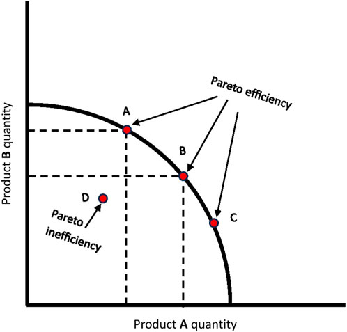
Figure 1. Visually represents a compromise solution in a multi-objective context, showcasing a balanced outcome that harmonizes conflicting criteria or goals without undue favouritism.
2.2 Notations
➢
➢
➢ R: number of objective functions.
➢
➢
➢
➢
➢
➢
➢
➢
➢
➢
➢
➢
➢
➢
➢
➢
➢
➢ ɸ: the feasible set of solution.
2.3 Mathematical model
A Multi-Objective Transportation Problem (MOTP) mathematical model entails utilizing math to build a structured representation of the problem’s complexity. Imagine this model as a blueprint that guides us through decision-making.
• Decision variables: Think of these as the key pieces we need to decide on. They tell us how much stuff goes from different places m (sources) to other places n (destinations). These sources could be factories, warehouses, or nodes in the supply chain, while destinations might be sales points or distribution centers.
• Objective functions: Imagine these as our goals. We might want to spend less money on transportation, keep our customers super happy, or make sure things are delivered quickly. We create equations to measure how well we’re achieving these goals.
• Constraints: These are rules we need to follow. We make sure that the total stuff leaving a source does not exceed what it has
• Transportation costs: These are the costs linked to moving things from one place to another. We use unknown variables (
This model helps us see the big picture, make smart decisions, and balance different objectives in a complex transportation problem.
Model 1
Subject to
We assume that
Model 2
Subject to
where
Assume that
Model 3
Subject to
We assume that
The multi-objective linear plus linear fractional transportation problem (MOLPLFTP) is a complex optimization challenge that involves optimizing the movement of resources from suppliers to consumers while considering both linear and linear fractional objectives. In this problem, the goals include minimizing transportation costs, maximizing customer satisfaction, or minimizing delivery time, and these objectives can have both linear and linear fractional components. The MOLPLFTP aims to find a solution that balances these conflicting objectives while efficiently allocating resources. This problem finds practical applications in supply chain management, logistics, and resource allocation, where multiple objectives need to be considered simultaneously. It is like solving a multi-layered puzzle that requires careful consideration of different goals and resource constraints to find the best possible outcome.
The implications of this study for industrial applications are significant:
• Optimal Decision-Making: Industries often face intricate transportation decisions involving multiple objectives and uncertainties. The study’s methodology can guide industries in making optimal decisions that consider various factors, leading to more efficient resource allocation and cost-effective solutions.
• Risk Management: Given that the study deals with stochastic problems and uncertain variables, its techniques can aid in risk management. Industries can use these methods to assess and mitigate the impact of uncertain events on transportation operations.
• Resource Utilization: The methodology assists industries in optimizing the allocation of resources such as raw materials, products, and transportation routes. This can lead to improved overall efficiency and reduced waste.
• Supply Chain Management: Transportation is a critical aspect of supply chain management. By incorporating stochastic programming and multi-objective optimization, industries can enhance the robustness and resilience of their supply chains.
• Adaptation to Changing Conditions: Industries often operate in dynamic environments where conditions change unpredictably. The study’s techniques provide a framework for adapting transportation strategies to evolving circumstances.
• Competitive Edge: Implementing advanced mathematical strategies for transportation problem-solving can provide industries with a competitive edge. More informed and optimized decisions can lead to increased customer satisfaction and cost savings.
• Decision Support System: The methodology described in the study can be integrated into decision support systems, aiding industries in real-time decision-making by considering uncertainty and multiple objectives.
• Sustainability Considerations: Industries are increasingly focused on sustainability. The study’s techniques can help in designing transportation strategies that minimize environmental impact and promote sustainable practices.
In essence, this study offers a roadmap for industries to navigate the complex and uncertain landscape of transportation challenges. By combining innovative mathematical strategies with advanced tools, industries can make informed, efficient, and effective decisions, even in the face of uncertainty. It is a valuable contribution that has the potential to transform the way industries approach transportation management.
3 Solution methodology
The constraints within the presented mathematical model, as detailed in Section 2, incorporate random values due to the consideration of the Weibull distribution. Consequently, direct solution using traditional mathematical techniques becomes infeasible. To address this challenge, the random constraints are ingeniously transformed into deterministic constraints, a transformation method elaborated upon in the following three scenarios outlined in Section 3.1. This transformation ensures that the inherent unpredictability in the constraints, attributed to the Weibull distribution, is effectively managed and incorporated into the optimization process.
3.1 Transformation techniques
The following scenarios need to be taken into account:
3.1.1. Only
3.1.2. Only
3.1.3. Both
3.1.1 Only
It is clarified that only the parameters
Certainly, the provided information clarifies the distribution and parameters associated with the independent random variables
or
Given by the probability density function of
Hence, the probabilistic constraint can be presented as:
The above integral can be expressed as:
Let,
The above constraint can be expressed as:
It can be integrated as:
On rearranging, we obtain
We have the logarithm in both directions
We obtain after decluttering and rearrangement
Then, as follows, the probabilistic constraints (2.1) can be changed into deterministic linear constraints:
The result is a multi-objective deterministic model, which in Model 4 below.
Model 4
Subject to
Where
3.1.2 Only
Only the parameters
The independent random variables
Given by the probability density function of
Hence, the probabilistic constraint can be presented as:
The above integral can be expressed as:
Let,
The above constraint can be expressed as:
It can be integrated as:
On rearranging, we obtain
We have the logarithm in both directions
We obtain after decluttering and rearrangement
Then, as follows, the probabilistic constraints (4.2) can be changed into deterministic linear constraints:
The result is a multi-objective deterministic model, which in Model 5 below.
Model 5
Subject to
Where
Both the independent random variables
Model 6
Subject to
Where
Various industrial issues can be modelled and solved using linear fractional stochastic transportation problems (LFTPs), a form of mathematical optimization problem. In an LFTP, where the cost of transportation is unpredictable, the objective is to minimize a linear fraction of those costs. This unpredictability may be caused by variables like shifting demand, unstable suppliers, or erratic production costs. A variety of industrial issues, such as production planning, inventory control, and supply chain management, can be modelled using LFTPs.
If we extend the above methodology for MOSLPLFTP. Then the model 3 can be converted into model 7 as
Model 7
Subject to
The MOSLPLFTP is an intricate mathematical challenge that addresses the optimization of resource movement between suppliers and consumers while considering multiple conflicting objectives, uncertainty, and a combination of linear and linear fractional goals. In this problem, objectives like minimizing costs, maximizing satisfaction, or minimizing delivery time can be both linear and linear fractional. Furthermore, uncertainties related to variables are taken into account. The MOSLPLFTP aims to find solutions that strike a balance between these conflicting objectives while adapting to uncertain conditions. This complex problem has practical applications in various areas, such as manufacturing process planning, supply chain management, transportation planning, and logistics, where efficient resource allocation while accommodating uncertainties is crucial. It is like solving a multi-dimensional puzzle, accounting for different goals and unknowns, to achieve optimal outcomes in complex scenarios.
A transportation problem known as a stochastic linear plus linear fractional transportation problem (SLPLFTP) contains stochastic parameters and an objective function that is a linear combination of two linear functions and a linear fractional function. This kind of issue can be used to address a number of manufacturing issues, including supply chain management, inventory management, and production process planning.
This study pioneer’s solutions for intricate transportation problems using advanced math and strategies. We introduce various approaches for addressing uncertainty with Weibull distribution in MOSLFTP and MOSLPLFTP. Stochastic programming and compromise techniques guide decision-making, while LINGO® 18.0 Software integrates methods. A practical example illustrates effectiveness, aiding decision-makers in complex scenarios.
4 Approaches to solve the MOLFTP and MOLPLFTP
These encompass mathematical optimization, where intricate formulations are analysed to achieve optimal solutions that align with multiple objectives while considering uncertainties. Complementing this, heuristic algorithms offer rapid approximate solutions by intelligently exploring solution spaces, particularly suitable for larger instances. Metaheuristic methods take the helm by employing sophisticated strategies like genetic algorithms and simulated annealing to navigate complex landscapes effectively. Simulation-based approaches step in, simulating real-world scenarios to comprehend the effects of various decisions under uncertain conditions. Lastly, interactive decision support systems offer an intuitive platform for decision-makers to visualize and assess different scenarios, thus untangling the complexity of MOSLFTP and MOSLPLFTP and facilitating well-informed choices.
4.1 Weighted sum method
For solving a Multi-Objective Linear Transportation Problem (MOLTP) the method of the weighted sum is highly used to obtain varying results for different weights. We use the extension of this method for our complex problems. The basic idea of this method is to assign weight
Subject to
The weights assigned to the objective function, denoted as
Peter C. Fishburn first put out the weighted sum approach in 1967 in his paper “Additive Utilities with Incomplete Product Set: Applications to Priorities and Assignments” (Fishburn, 1967). The weighted sum approach was found to be a quick and efficient way by Fishburn to create a mechanism for making decisions based on several factors.
Since then, one of the most popular techniques for multi-criteria decision-making (MCDM) is the weighted sum method. It is employed in many various industries, including business, engineering, and government. The weighted sum method can be applied to a variety of MCDM problems and is reasonably simple to apply. It is crucial to remember that the weighted sum method is only as effective as the weights chosen. The proportional importance of each criterion to the decision-maker should be carefully reflected in the weights.
4.2 Proposed method
Joshi (Joshi et al., 2022b) introduced a model aimed at deriving a compromise solution for a Multi-Objective Linear Transportation Problem (MOLTP). This approach centres on the transformation of the multi-objective optimization problem into a new single-objective optimization, emphasizing the attainment of a balanced outcome.
Where
Subject to
The collection of workable options is called X, and x is an n-dimensional decision-maker variable. Each objective is transformed into constraints with an upper bound of
The problem reduces as:
Subject to
Here in this model a factor
In a situation where there are multiple criteria to consider, solutions are evaluated using a method based on ratios. This method compares each solution to an ideal one and an anti-ideal one. The ratio helps measure how close a solution is to the ideal and how far it is from the anti-ideal. The compromise solution with the highest ratio effectively balances these factors, taking into account conflicting criteria when making decisions.
The diversity of approaches for tackling multi-objective transportation problems necessitates a means of ranking these methods to aid in their selection. To address this challenge, a tool is required to assist in the ranking and identification of the most suitable method. At this juncture, the Technique for Order of Preference by Similarity to the Ideal Solution (TOPSIS) (Rizk-Allah et al., 2018) emerges as a valuable asset. TOPSIS serves the purpose of ranking different methods based on the performance of their optimal solutions. In this context, the alternatives refer to the optimal solutions, while the criteria pertain to the objective functions. Essentially, TOPSIS enables us to discern which method proves most effective in terms of achieving optimal solutions for the specific problem under consideration.
4.3 Step by step implementation of proposed approach
1. Start: The beginning of the process.
2. Create required mathematical model as specified in Section 3. This involves formulating the problem mathematically, considering all relevant constraints and objectives.
3. Solve each objective separately: To understand the performance of each objective independently, solve them one by one.
4. Check if the separately obtained solutions for each objective are the same: Verify whether the solutions obtained for individual objectives align or differ. This step helps in assessing any conflicts or trade-offs between objectives.
5. Evaluate each objective function: Calculate the values of each objective function to determine their individual contributions to the overall problem.
6. Establish the weights for the objectives: Assign weights to each objective to reflect their relative importance in the decision-making process. This step involves considering the preferences and priorities of the decision-maker.
7. Construct the proposed model and solve it: Create a model that combines all objectives with their respective weights and solve it to find a solution that balances these objectives.
8. Evaluate each objective function for the outcome of the model’s solution: Assess the performance of each objective based on the solution obtained from the combined model.
9. The compromise solution has been attained: This indicates that a solution has been reached, which is a compromise between conflicting objectives.
10. If the decision-maker (DM) is satisfied, move on to the next step; otherwise, return to step 7. If the DM is not satisfied with the compromise solution, the process is iterated to find a more acceptable solution.
11. Rank and compile a list of the best solutions for different transportation problems using the TOPSIS approach. This step (Figure 2) involves comparing various solutions based on their performance against the objectives and ranking them accordingly.
12. Stop: The conclusion of the process.
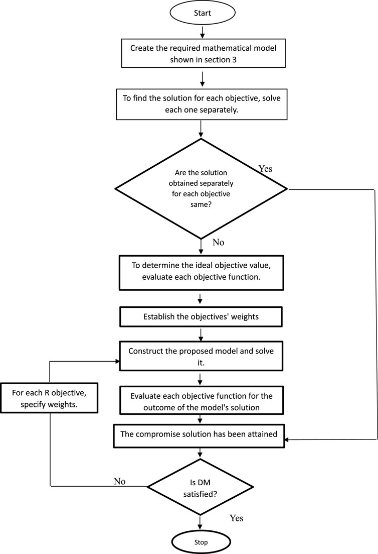
Figure 2. Flow chart for the proposed method.
This structured approach ensures that multiple objectives are considered, a compromise solution is achieved, and a ranking of solutions is provided when necessary, offering a comprehensive methodology for addressing complex transportation optimization problems.
5 Numerical illustration
This section exemplifies the tangible impact of our MOSLFTP and MOSLPLFTP research, unveiling its practicality through numerical demonstrations. In Section 3, we introduced MOSLFTP and MOSLPLFTP models and, employing our method alongside the weighted sum approach, derived optimal compromise solutions. The deterministic equivalents of these mathematical models were implemented using the Lingo 18.0 solver, grounding our research in real-world applicability.
In this illustrative section, we immerse ourselves in a practical scenario within the realm of Third-Party Logistics (TPL). Picture a dynamic transportation network where a TPL company plays a pivotal role. This network features four suppliers, symbolized as source nodes:
In this dynamic environment, the supply of fresh goods experiences variability influenced by uncontrollable factors like weather conditions and labour availability at the farms. This unpredictability transforms the availability of such produce into a probabilistic phenomenon, particularly when supply stability is uncertain. Consequently, the likelihood of obtaining the desired quantity of produce from provider a₁ is represented by
The demand for fresh fruit is naturally unpredictable. Inaccurate demand forecasts, demand volatility, or unanticipated delivery delays are the main causes. Therefore, the chance that the anticipated demand is necessary for market hall
5.1 Numerical example 1 (MOSLFTP)
Subject to
(Feasibility condition)
Where
Tables 2, 3 shows the values of

Table 2. Specified probability level values for supplies

Table 3. Specified probability level values for supplies
Using the data table provided in Tables 2–5, the following two-objective deterministic TP is formulated as:

Table 4. Data of transportation cost.

Table 5. Data of transportation profit.
Subject to
5.2 Numerical example 2 (MOSLPLFTP)
Using the data provided in Tables 4–8, the following two-objective deterministic TP is formulated as:

Table 6. Data of transportation time.

Table 7. Specified probability level values for supplies

Table 8. Specified probability level values for supplies
Subject to
5.3 Numerical example 3 (MOSLPLFTP)
Using the data provided in Tables 9–13 the following three-objective deterministic TP is formulated as:

Table 9. Data of transportation time.

Table 10. Data of transportation cost.

Table 11. Data of transportation profit.

Table 12. Specified probability level values for supplies

Table 13. Specified probability level values for supplies
Subject to
5.4 Multi-objective stochastic linear fractional transportation problem (numerical example 1)
5.5 Multi-objective stochastic linear plus linear fractional transportation problem (numerical example 2)
5.6 Multi-objective stochastic linear plus linear fractional transportation problem (numerical example 3)
6 Result and discussion
The LINGO® 18.0 Software is used to tackle numerical examples according to the proposed mathematical programming model in previous section. Objectives have been solved separately in Tables 14–16. The objectives are listed separately in Tables 14–16. Where the ideal values
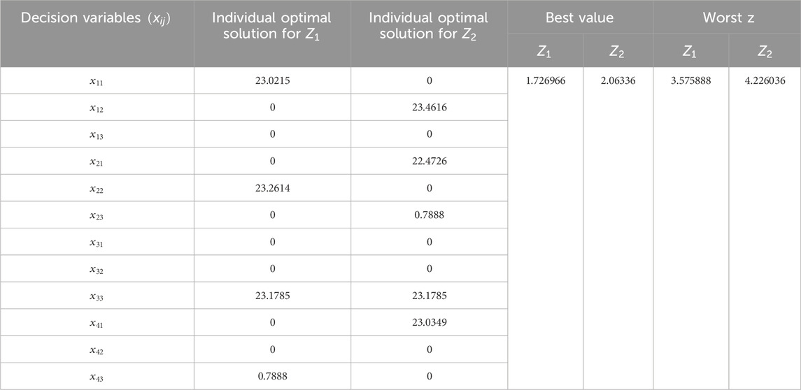
Table 14. The solutions obtained for both the objectives separately, ignoring other objectives.
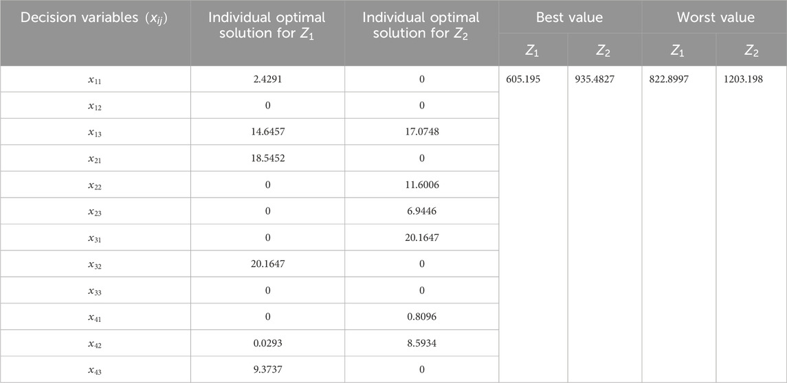
Table 15. The solutions obtained for both objectives separately, ignoring other objectives.
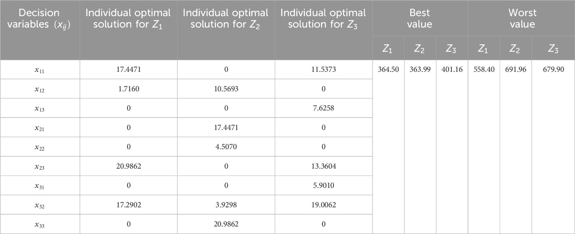
Table 16. The solutions obtained for all three objectives separately, ignoring other objectives.
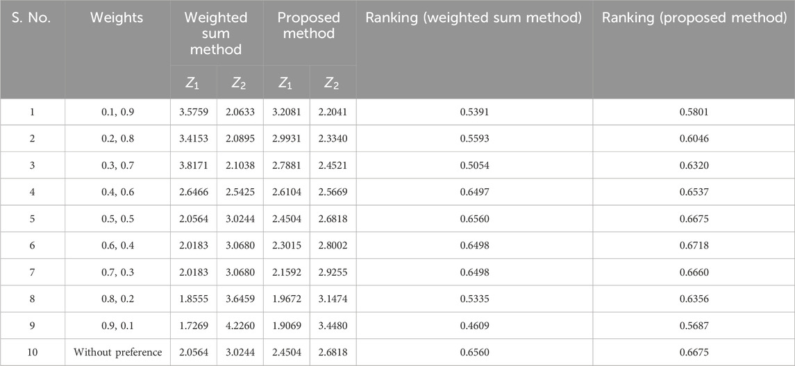
Table 17. Comparison of solution of numerical example 1 by weighted sum and the proposed method.
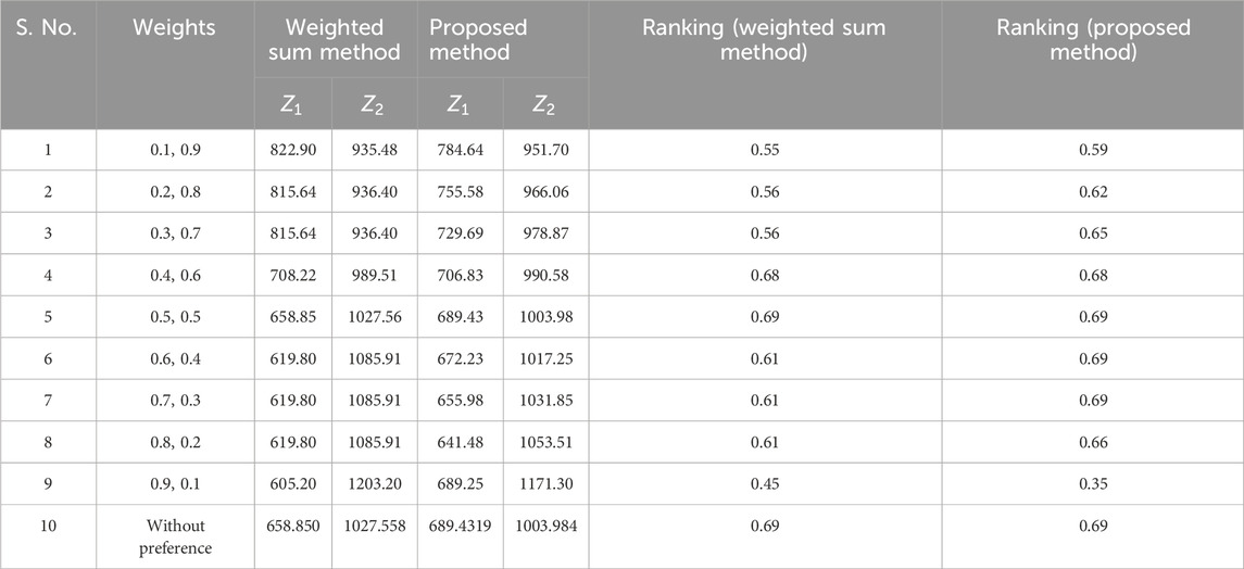
Table 18. Comparison of solution of numerical example 2 by weighted sum and proposed Method.
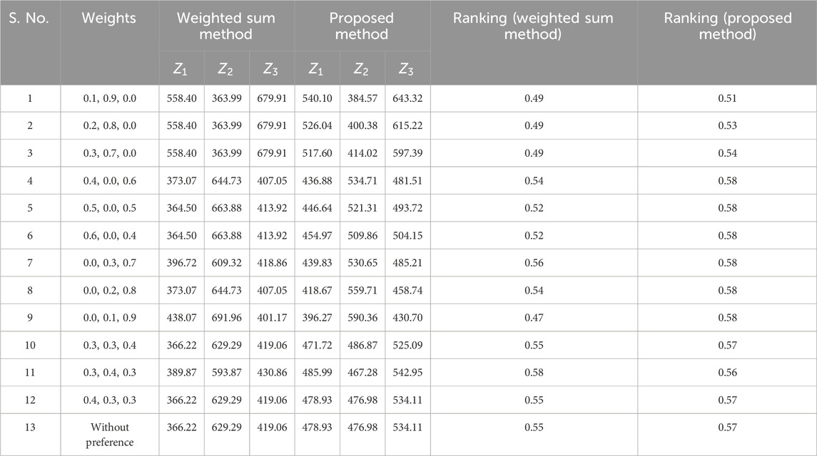
Table 19. Comparison of solution of numerical example 3 by weighted sum and proposed Method.
Creating a graph to vividly illustrate the comparative performance of the Weighted Sum Method and our innovative Proposed Method, akin to a dynamic duel. Graph that compares the weighted sum method and our new proposed method. This graph shows how they rank, like who’s doing better. We can see that our proposed method is closer to the best solution. It is like a race, and our method is winning by being closer to what we want. The graph is like a storyteller that tells us our method is good at finding the right answers. Figures 3–5 represents the ranking comparison of MOSLFTP/MOSLPLFTP between proposed approach with the weighted sum method.
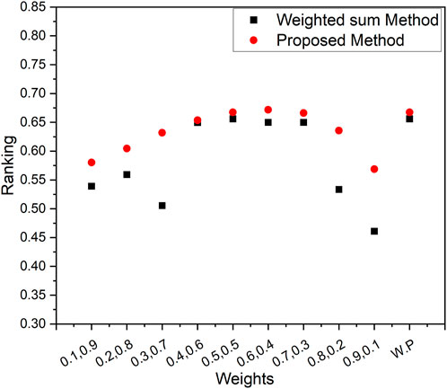
Figure 3. Graphical representation of ranking comparison between the weighted sum method and the proposed method for numerical example 1.
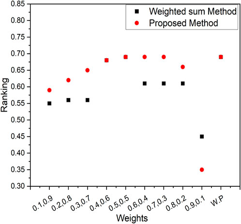
Figure 4. Graphical representation of ranking comparison between the weighted sum method and the proposed method for numerical example 2.
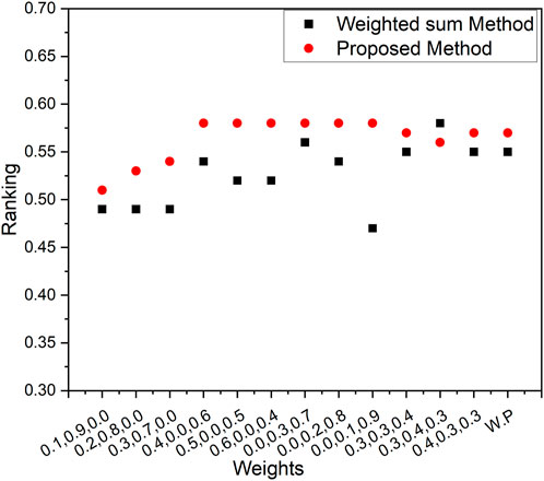
Figure 5. Graphical representation of ranking comparison between the weighted sum method and the proposed method for numerical example 3.
7 Conclusion
In conclusion, this paper ushers in a new era of innovation in transportation problem-solving for recent manufacturing process scenarios. By introducing the concept of the MOSLFTP and harnessing the power of stochastic programming, the study offers industries a transformative approach to navigating uncertainty and complexity. The utilization of compromise programming stands as a testament to the paper’s practicality, addressing the challenges of conflicting objectives in transportation management. The seamless integration of the MOSLPLFTP through LINGO® 18.0 Software demonstrates a tangible bridge between theory and application. The paper’s highlighted example magnificently showcases the methodology’s efficacy in real-world scenarios, guiding decision-makers through the intricate terrain of uncertainty. This study is an invaluable compass for industries, steering them toward well-informed choices and setting a course for success amidst the tumultuous seas of contemporary challenges in transportation. Within the pages of this paper, we employed a ranking approach to gauge our method’s effectiveness. It is like lining up solutions and figuring out how close they are to the best one. Our approach stands out—it is like we found a sweet spot, a solution that’s close to what we want. It is like finding the perfect compromise. This journey has shown that our method is not just good, it is the best way to find a solution that balances different goals. It is like hitting the bullseye, and we’ve uncovered a solution that’s as close to perfect as it gets. Imagine this paper as a helpful tool, like a magical compass, showing manufacturing industries the way through the maze of tricky transportation decisions. It is like having a secret weapon to tackle challenges and reach success in the ever-changing world of transportation. In the future, we can extend this work for the multi-choice multi-objective interval stochastic transport problem with mixed constraints, applying Lagrange’s or Newton’s divided difference approaches.
Data availability statement
The raw data supporting the conclusion of this article will be made available by the authors, without undue reservation.
Ethics statement
The manuscript presents research on animals that do not require ethical approval for their study.
Author contributions
VJ: Writing–review and editing, Writing–original draft, Visualization, Validation, Supervision, Software, Resources, Project administration, Methodology, Investigation, Funding acquisition, Formal Analysis, Data curation, Conceptualization, Writing–review and editing, Writing–original draft, Visualization, Validation, Supervision, Software, Resources, Project administration, Methodology, Investigation, Funding acquisition, Formal Analysis, Data curation, Conceptualization, MS: Writing–review and editing, Visualization, Validation, Software, Resources, Methodology, Investigation, Formal Analysis, Writing–review and editing, Visualization, Validation, Software, Resources, Methodology, Investigation, Formal Analysis, AK: Writing–review and editing, Visualization, Validation, Supervision, Project administration, Investigation, Funding acquisition, Formal Analysis, Conceptualization, Writing–review and editing, Visualization, Validation, Supervision, Project administration, Investigation, Funding acquisition, Formal Analysis, Conceptualization, LC: Writing–review and editing, Visualization, Validation, Supervision, Resources, Funding acquisition, Conceptualization, Writing–review and editing, Visualization, Validation, Supervision, Resources, Funding acquisition, Conceptualization, RK: Writing–review and editing, Project administration, Methodology, Writing–review and editing, Project administration, Methodology, ND: Writing–review and editing, Formal Analysis, Data curation, Writing–review and editing, Formal Analysis, Data curation.
Funding
The author(s) declare that no financial support was received for the research, authorship, and/or publication of this article.
Conflict of interest
The authors declare that the research was conducted in the absence of any commercial or financial relationships that could be construed as a potential conflict of interest.
Publisher’s note
All claims expressed in this article are solely those of the authors and do not necessarily represent those of their affiliated organizations, or those of the publisher, the editors and the reviewers. Any product that may be evaluated in this article, or claim that may be made by its manufacturer, is not guaranteed or endorsed by the publisher.
References
Boadh, R., Chaudhary, K., Dahiya, M., Dogra, N., Rathee, S., Kumar, A., et al. (2022). Analysis and investigation of fuzzy expert system for predicting the child anaemia. Mater Today Proc. 56, 231–236. doi:10.1016/j.matpr.2022.01.094
Buvaneshwari, T. K., and Anuradha, D. (2022). Solving stochastic fuzzy transportation problem with mixed constraints using the Weibull distribution. J. Math. 11, 1–11. doi:10.1155/2022/6892342
Charles, V., and Dutta, D. (2005). Linear stochastic fractional programming with sum of probabilistic fractional objective. https://optimization-online.org/?p=9758
Dantzig, G. B. (1963). Linear programming and extensions. Princeton, NY, USA: Princeton University Press.
Dantzig, G. B. (2011). Linear programming under uncertainty. Stoch. Program 150. doi:10.1287/mnsc.1.3-4.197
Das, A., and Lee, G. M. (2021). A multi-objective stochastic solid transportation problem with the supply, demand, and conveyance capacity following the Weibull distribution. Mathematics 9 (15), 1757. doi:10.3390/math9151757
Fishburn, P. C. (1967). Letter to the editor—additive utilities with incomplete product sets: application to priorities and assignments. Oper. Res. 15 (3), 537–542. doi:10.1287/opre.15.3.537
Goicoechea, A., and Duckstein, L. (1987). Nonnormal deterministic equivalents and a transformation in stochastic mathematical programming. Appl. Math. Comput. 21 (1), 51–72. doi:10.1016/0096-3003(87)90009-9
Jadhav, V. A., and Doke, D. M. (2016). Solution procedure to solve fractional transportation problem with fuzzy cost and profit coefficients. Int. J. Math. 4 (7), 1554–1562.
Jain, S., and Arya, N. (2013). An inverse transportation problem with the Linear fractional objective function. Adv. Model Optim. 15 (3), 677–687.
Javaid, S., Jalil, S. A., and Asim, Z. (2017). A model for uncertain multi-objective transportation problem with fractional objectives. Int. J. Oper. Res. 14 (1), 11–25.
Joshi, V. D., Agarwal, K., and Singh, J. (2022b). Goal programming approach to solve linear transportation problems with multiple objectives. J. Comp. Anal. Appl. 31 (1), 127–139.
Joshi, V. D., Saini, R., Singh, J., and Nisar, K. S. (2022a). Solving multi-objective linear fractional transportation problem under neutrosophic environment. J. Interdiscip. Math. 25 (1), 123–136. doi:10.1080/09720502.2021.2006327
Koopmans, T. C. (1949). Optimum utilization of the transportation system. Econometrica 17, 136–146. doi:10.2307/1907301
Krishnamoorthy, K. (2006). Handbook of statistical distributions with applications. New York, NY, USA: Chapman and Hall/CRC Press.
Kumar, A., and Gulati, V. (2021). Optimization and investigation of process parameters in single point incremental forming. Indian J. Eng. Mater Sci. (IJEMS). 27 (2), 246–255. doi:10.56042/ijems.v27i2.45925
Kumar, A., Kumar, D., Kumar, P., and Dhawan, V. (2020). Optimization of incremental sheet forming process using artificial intelligence-based techniques. Nat-Inspired Optim. Adv. Manuf. Process Syst., 41 113–130. doi:10.1201/9781003081166
Kumar, A., Kumar, V., Modgil, V., and Kumar, A. (2022). Stochastic Petri nets modelling for performance assessment of a manufacturing unit. Mater Today Proc. 56, 215–219. doi:10.1016/j.matpr.2022.01.073
Kumar, A., Kumar Mittal, P., and Gambhir, V. (2023b). Materials processed by additive manufacturing techniques, Advances in additive manufacturing artificial intelligence, 23. doi:10.1016/B978-0-323-91834-3.00014-4
Kumar, A., Singh, H., Kumar, P., and AlMangour, B. (2023a). Handbook of Smart manufacturing: forecasting the future of Industry 4.0. doi:10.1201/9781003333760
Nasseri, S. H., and Bavandi, S. (2020). Solving multi-objective multi-choice stochastic transportation problem with fuzzy programming approachintelligent Syst. (CFIS), 2020. doi:9238695doi:10.1109/CFIS49607.2020.9238695
Pradhan, A., and Biswal, M. P. (2015). “Computational methodology for linear fractional transportation problem,” in (IEEE Publications), 23, 3158–3159. doi:10.1109/WSC.2015.7408448
Rizk-Allah, R. M., Hassanien, A. E., and Elhoseny, M. (2018). A multi-objective transportation model under neutrosophic environment. Comput. Electr. Eng. 69, 705–719. doi:10.1016/j.compeleceng.2018.02.024
Roy, S. K. (2014). Multi-choice stochastic transportation problem involving Weibull distribution. Int. J. Oper. Res. 21 (1), 38–58. doi:10.1504/IJOR.2014.064021
Sadia, S., Gupta, N., and Ali, Q. (2016). Multi-objective capacitated fractional transportation problem with mixed constraints. Math. Sci. Lett. 5 (3), 235–242. doi:10.18576/msl/050304
Safi, M., and Seyyed, M. G. (2017). Uncertainty in linear fractional transportation problem. Int. J. Nonlinear Anal. Appl. 8 (1), 81–93. doi:10.22075/IJNAA.2016.504
Saini, R., Joshi, V. D., and Singh, J. (2022). On solving a MFL paradox in linear plus linear fractional multi- objective transportation problem using fuzzy approach. Int. J. Appl. Comp. Math. 8, 79. doi:10.1007/s40819-022-01278-5
Swarup, K. (1966). Transportation technique in linear fractional functional programming. Jr. Nav. Sci. Serv. 21 (5), 256–260.
Yadav, A. S., Kumar, A., Yadav, K. K., and Rathee, S. (2023). Optimization of an inventory model for deteriorating items with both selling price and time-sensitive demand and carbon emission under green technology investment. Int. J. Interact. Des. Manuf. (IJIDeM), 56, 1–17. doi:10.1007/s12008-023-01689-8
Keywords: multi-objective decision-making, transportation problem, fractional programming, manufacturing process, modelling and simulation, uncertainty, soft computing
Citation: Joshi VD, Sharma M, Kumar A, Cepova L, Kumar R and Dogra N (2024) Navigating uncertain distribution problem: a new approach for resolution optimization of transportation with several objectives under uncertainty. Front. Mech. Eng 10:1389791. doi: 10.3389/fmech.2024.1389791
Received: 22 February 2024; Accepted: 07 March 2024;
Published: 04 April 2024.
Edited by:
Kanak Kalita, Vel Tech Dr. RR and Dr. SR Technical University, IndiaReviewed by:
Sachin Salunkhe, Gazi University, TürkiyeVishwanatha H. M., Manipal Institute of Technology, India
Poonam Chaudhary, The Northcap University, India
Copyright © 2024 Joshi, Sharma, Kumar, Cepova, Kumar and Dogra. This is an open-access article distributed under the terms of the Creative Commons Attribution License (CC BY). The use, distribution or reproduction in other forums is permitted, provided the original author(s) and the copyright owner(s) are credited and that the original publication in this journal is cited, in accordance with accepted academic practice. No use, distribution or reproduction is permitted which does not comply with these terms.
*Correspondence: Ajay Kumar, YWpheS5rdW1hcjMwODg2QGdtYWlsLmNvbQ==; Lenka Cepova, bGVua2EuY2Vwb3ZhQHZzYi5jeg==;