On the generalization discrepancy of spatiotemporal dynamics-informed graph convolutional networks

Graph neural networks (GNNs) have gained significant attention in diverse domains, ranging from urban planning to pandemic management. Ensuring both accuracy and robustness in GNNs remains a challenge due to insufficient quality data that contains sufficient features. With sufficient training data where all spatiotemporal patterns are well-represented, existing GNN models can make reasonably accurate predictions. However, existing methods fail when the training data are drawn from different circumstances (e.g., traffic patterns on regular days) than test data (e.g., traffic patterns after a natural disaster). Such challenges are usually classified under domain generalization. In this work, we show that one way to address this challenge in the context of spatiotemporal prediction is by incorporating domain differential equations into graph convolutional networks (GCNs). We theoretically derive conditions where GCNs incorporating such domain differential equations are robust to mismatched training and testing data compared to baseline domain agnostic models. To support our theory, we propose two domain-differential-equation-informed networks: Reaction-Diffusion Graph Convolutional Network (RDGCN), which incorporates differential equations for traffic speed evolution, and the Susceptible-Infectious-Recovered Graph Convolutional Network (SIRGCN), which incorporates a disease propagation model. Both RDGCN and SIRGCN are based on reliable and interpretable domain differential equations that allow the models to generalize to unseen patterns. We experimentally show that RDGCN and SIRGCN are more robust with mismatched testing data than state-of-the-art deep learning methods.

1 Introduction

Spatiotemporal prediction is a key task in many scientific and engineering domains, ranging from structural health monitoring (Morid et al., 2023), evolution of microstructures (Montes de Oca Zapiain et al., 2021), traffic management (Bui et al., 2022), weather forecasting (Longa et al., 2023), and disease control (Jayatilaka et al., 2020). With explosive growth in data collection technologies and sufficient training data, deep learning approaches (Yu et al., 2018; Wu et al., 2020) have come to dominate the field of data-driven prediction of complex systems. Among best-performing models, graph neural networks (GNNs) dominate due to their ability to incorporate spatiotemporal information (Han et al., 2021; Shang et al., 2021; Ji et al., 2022) so that dependent information at different locations and times can be captured and exploited to make more accurate predictions. However, as these models grow more complex, thus requiring substantial training data, their performance when test conditions are different from training conditions has been shown to be weak. The collection of data from all representative conditions is almost impossible in many domains, and so there is a need to develop methods for data-driven prediction that can handle this generalization.

Such challenges are usually classified under “domain generalization” (Figure 1), where a model is trained on a source domain but evaluated on a target domain with different characteristics (mismatches). Consider traffic speed prediction as a motivating example. It is well known that prediction algorithms perform poorly when traffic patterns are unexpectedly disrupted, for instance, due to extreme weather, natural disasters, or even special events. In our evaluation section, we will demonstrate this phenomenon more concretely, where state-of-the-art deep learning methods do not generalize well when dataset patterns are split between training (weekday) and test patterns (weekend). The challenge mentioned above can be formulated as learning with mismatched training data (Varshney, 2020), a problem that is often encountered in practice.

Figure 1

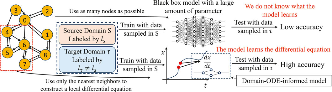
Figure 1. Training and test sets consist of a source domain S characterized by a labeling function l_s, and a target domain τ distinguished by a different labeling function l_τ ≠ l_s. Data collection in the source domain is convenient, whereas acquiring data in the target domain is challenging and often only feasible at test time. Without integrating a domain ODE, a model, despite having numerous parameters, may experience diminished accuracy when tested with such mismatched patterns. Conversely, employing an architecture that integrates a domain ODE enables the model to capture local patterns and attain high accuracy even with previously unseen patterns, while requiring fewer parameters.

This leads to the main hypothesis of our paper: when scientific equations or physical models are available to capture the local spatiotemporal dynamics of vertices in a network, such that these dynamics remain consistent between training and test conditions, then machine learning models that incorporate these scientific equations can lower the generalization discrepancy of the learned model. In particular, we consider systems where local dynamics are available in the form of ordinary differential equations, which we use to construct a novel graph-convolution network structure for spatiotemporal prediction. We will use a known probably approximately correct (PAC) learning approach to quantify generalization discrepancy between predictions under different source and target labeling functions, proving mathematically that under certain learnability and symmetry assumptions on the labeling functions, incorporating the local dynamics can lower the discrepancy. We operationalize our approach by constructing two different dynamics-informed GCNs for application in traffic-speed prediction and influenza-like-illness (ILI) prediction using domain ordinary differential equations (ODEs). Our novel domain-ODE-informed neural networks called “Reaction-Diffusion Graph Convolutional Network” (RDGCN), and “Susceptible-Infectious-Recovered Graph Convolutional Network” (SIRGCN) augment GCNs with domain ODEs studied in transportation research (Bellocchi and Geroliminis, 2020) and disease epidemics (Stolerman et al., 2015). Through experimental evaluation on real datasets, we demonstrate that our novel-dynamics-informed GCNs are more robust in situations with data mismatches than baseline models in traffic speed prediction and influenza-like illness prediction. Furthermore, the prior knowledge encoded by the dynamics-informed architecture reduces the number of model parameters, thus requiring less training data. The model computations are better grounded in domain knowledge and are thus more accessible and interpretable for domain experts.

We highlight our contributions as follows:

• We study the challenge of graph-time-series prediction with mismatched data where the patterns in the training set are not representative of those in the test set.

• We theoretically prove the robustness of domain-ODE-informed GCNs to a particular form of domain generalization when the labeling function differs between the source and target domains. Specifically, we show that the generalization discrepancy is lower for the domain-ODE-informed learning model under certain conditions than a domain-independent learning model.

• We develop two novel domain-ODE-informed neural networks called “Reaction-Diffusion Graph Convolutional Network” (RDGCN), and “Susceptible-Infectious-Recovered Graph Convolutional Network”(SIRGCN) that augment GCNs with domain ODEs studied in transportation research (Bellocchi and Geroliminis, 2020) and disease epidemics (Stolerman et al., 2015).

• By conducting experimental assessments on authentic datasets, we illustrate that our innovative dynamics-informed GCNs exhibit greater robustness in scenarios featuring data mismatches than baseline models in both traffic speed prediction and influenza-like illness prediction.

• By integrating domain difference equations, the dynamics-informed GCNs can substantially decrease the quantity of model parameters, resulting in reduced training data requirements and accelerated training and inference processes.

The structure of this paper unfolds as follows. In Section 2, we provide a comprehensive background on graph neural networks (GNNs) for time-series prediction, elucidating the challenges encountered in achieving domain generalization within GNNs. Section 3 formalizes the problem by defining the generalization discrepancy between the source and target domains. Building upon this, Section 4 details our proposed methodology, introducing a novel approach that integrates domain differential equations into GCNs. Here, we outline the architecture of dynamics-informed graph convolutional networks (DGCNs), specifically tailored for spatiotemporal prediction tasks. The theoretical underpinnings of our approach are rigorously examined in Section 5, where we explore the generalization properties of DGCNs. Additionally, theoretical bounds on the discrepancy between source and target domains are derived. Section 6 showcases the practical application of DGCNs on real-world datasets, focusing on two case studies: RDGCN for predicting traffic speed evolution and SIRGCN for modeling disease propagation. Through these applications, we evaluate the effectiveness of DGCNs in mitigating the generalization gap. To further bolster our claims, Section 7 and 8 detail the experimental setup, results obtained, and an ablation study. These sections offer additional insights into the performance of RDGCN and SIRGCN, further validating our proposed methodology. In Section 9, we assess the model complexity of RDGCN and SIRGCN. Finally, in Section 10, we draw conclusions by summarizing the key findings and implications of our research. Additionally, we propose potential avenues for future research aimed at enhancing the generalization capabilities of DGCNs in the realm of time-series predictions.

2 Related work

2.1 Graph neural networks on time series predictions

GNNs have been widely utilized to enable great progress in dealing with graph-structured data (Kipf and Welling, 2017; Yu et al., 2018; Li et al., 2018; Cui et al., 2020) build spatiotemporal blocks to encode spatiotemporal features (Wu et al., 2020; Shang et al., 2021; Han et al., 2021; Veličković et al., 2018; Guo et al., 2019) and generate dependency graphs which only focus on “data-based” dependency where features at a vertex can be influenced by a vertex but not in its physical vicinity. None of these approaches exploit domain ODEs for better generalization and robustness.

2.2 Domain generalization

Domain generalization has gained increasing attention recently (Wang et al., 2022; Zhou et al., 2022; Robey et al., 2021; Zhou et al., 2021), and robustness to domain data with mismatched patterns is important in designing trustworthy models (Varshney, 2020). The goal is that a model learns to generalize to unseen domains. Many studies (Robey et al., 2021) assume that there is an underlying transformation between the source and target domain and use an extra model to learn the transformations (Xian et al., 2022); therefore, the training data must be sampled under at least two individual distributions. However, our approach addresses this challenge by incorporating a domain-specific ODE instead of using extra training processes that learn from the data from two individual domains or employing additional assumptions on transformations, thus working for arbitrary domain scenarios.

2.3 Domain dynamics, differential equations and neural ODEs

Time series are modeled using differential equations in many areas, such as chemistry (Scholz and Scholz, 2015) and transportation (van Wageningen-Kessels et al., 2015; Loder et al., 2019; Kessels and Kessels, 2019). These approaches focus on equations that reflect the most essential relationships. To incorporate differential equations into machine learning, many deep learning models based on neural ODEs (Chen et al., 2018; Jia and Benson, 2019; Asikis et al., 2022) have been proposed. Advancements extend to graph ODE networks (Ji et al., 2022; Choi et al., 2022; Jin et al., 2022) which use black-box differential equations to simulate continuous traffic-pattern evolution. However, the potential of domain knowledge to fortify algorithmic robustness against domain generalization has yet to be explored.

2.4 Integrating domain knowledge into deep learning

Incorporating domain knowledge in deep learning has been garnering growing interest (Van Der Voort et al., 1996; Chen et al., 2011; Kumar and Vanajakshi, 2015; Thodi et al., 2022). For example, Physics-Informed Neural Network (PINN) approaches (Raissi et al., 2019; Karniadakis et al., 2021) incorporate physics equations to augment deep learning. PINN has been extended to incorporate a macroscopic traffic model (Huang and Agarwal, 2020) to enhance learning in traffic state prediction. However, the integration of traffic models with the graphical structure of the transportation network has not been explored, particularly in the context of mismatched data.

2.5 Limited and mismatched data

Meta-learning (Finn et al., 2017) is often used to augment machine learning with limited data, through additional training processes. Mismatches between the training and test sets are frequently present in practical applications. Robustness to mismatched data is important in designing trustworthy models (Varshney, 2020). The optimization of supervised learning when the instance/label pairs have been permuted in a manner is proposed in Xian et al. (2022). Our approach, which incorporates domain ODEs, provides robustness under arbitrarily mismatch and limited data scenarios.

2.6 Model explainability

Intrinsically transparent ML models (Lakkaraju et al., 2016; Lou et al., 2012) based on simple rules or linear models are useful, in that their computation processes can be revealed to domain experts to increase model confidence. In contrast, we incorporate non-linear physical laws into graphical models to promote intrinsic explainability. In graph-based ML, understanding how neighbors lead to prediction on a mode is essential. Prior methods, such as Ying et al. (2019), use a surrogate model to approximate a graphical model and thus do not reveal the computational process of prediction models.

3 Problem definition

3.1 Notations

Given an unweighted graph $\mathcal{G}=(\mathcal{V},\mathcal{E})$ with $|\mathcal{V}|=n$ vertices and $|\mathcal{E}|$ edges, each vertex $i\in \mathcal{V}$ corresponds to a physical location, and each edge $(i,j)\in \mathcal{E}$ represents the neighboring connectivity between two vertices. Let ${\mathcal{N}}_i$ denote the set of neighbors of vertex i, and $\mathcal{A}\in {\mathbb{R}}^{n\times n}$ denote the adjacency matrix of the graph $\mathcal{G}$. The value of the feature at vertices i at time t is denoted x_i(t), and the vector of features at all vertices at time t is denoted X(t). Let $X_{t_1:t_2}\in {\mathbb{R}}^{n\times (t_2-t_1)}$ be the sequence of features X (t₁), X (t₁ + 1), …, X (t₂) at all vertices in the interval [t₁, t₂]. Assume that the training and test data are sampled from the source ${\mathcal{X}}_s$ and target domains ${\mathcal{X}}_{\tau }$, respectively. Data from different domains exhibit different patterns, which we explicitly capture through labeling functions in each domain. Formally

${\mathcal{X}}_s=\left\{\left(X_{t-T:t},X_{t+1}\right):X_{t+1}=l_s\left(X_{t-T:t}\right),X_{t-T:t}\sim \mathcal{D}\right\},$

where l_s is the labeling function in the source domain and $\mathcal{D}$ is the distribution of inputs. The target domain ${\mathcal{X}}_{\tau }$ can be defined similarly but with a different labeling function l_τ ≠ l_s. Note that T is the length of the time sequence that defines the “ground truth” labeling function, which we assume to be partially known at best. We assume that T is identical in the source and target domains.

3.2 Problem definition

We aim to solve the problem of single domain generalization (Qiao et al., 2020; Wang et al., 2021; Fan et al., 2021). Given the past feature observations denoted as $(X_{t-T:t}^s,X_{t+1}^s)\in {\mathcal{X}}_s$ on the graph $\mathcal{G}$ on only one source domain s, we aim to train a predictive hypothesis h that can predict the feature at time t + 1 for all vertices (denoted as $\widehat{X}(t+1)\in {\mathbb{R}}^n$) on the unseen target domain τ without extra training. We use L to denote a loss function to evaluate the distance between the prediction and ground truth. Let h denote a hypothesis, and let l denote the labeling function in the corresponding domain. The expectation of the loss is ${\mathcal{L}}_{(\mathcal{D},l)}(h)={\mathbb{E}}_{X_{t-T:t}\sim \mathcal{D}}(L(h(X_{t-T:t}),l(X_{t-T:t})))$. The hypothesis returned by the learning algorithm is

$h^{*}=\underset{h\in \mathcal{H}}{\mathrm{argmin}}{\mathcal{L}}_{\left(\mathcal{D},l_s\right)}\left(h\right),$

where $\mathcal{H}$ is any hypotheses set. Let ${\mathcal{H}}^{*}$ denote the set of hypotheses returned by the algorithm—${\mathcal{H}}^{*}=\{h^{*}:{\mathcal{L}}_{(\mathcal{D},l_s)}(h^{*})<ϵ\}$—and define the discrepancy measure that quantifies the divergence between the source and target domain as (Kuznetsov and Mohri, 2016):

$disc\left({\mathcal{H}}^{*}\right)=\underset{h\in {\mathcal{H}}^{*}}{\sup }|{\mathcal{L}}_{\left(\mathcal{D},l_s\right)}\left(h\right)-{\mathcal{L}}_{\left(\mathcal{D},l_{\tau }\right)}\left(h\right)|.(1)$

Our objective is to develop a class of learning architectures to train a hypothesis that has low generalization discrepancy as measured above. Our approach, as delineated in the next section, will focus on the use of graph convolutional network architectures that incorporate the local spatiotemporal dynamics available in the form of ODEs.

4 Methodology

Let x_i(t) denote a feature at vertex i at time t and $H_{t,T}^i$ denote the length T history of data prior to time t, and set ${\mathcal{N}}_i$ of 1-hop neighbors of vertex i. The ODE that models the feature dynamics at vertex i is given by

$\frac{d{x}_i\left(t\right)}{dt}=f_i\left(x_i\left(t\right),\left\{x_j\left(t\right)|j\in {\mathcal{N}}_i\right\}\right)+g_i\left(H_{t,T}^i\right),(2)$

where $f_i(x_i(t),\{x_j(t)|j\in {\mathcal{N}}_i\})$ models the evolution of the feature (Asikis et al., 2022; Xhonneux et al., 2020) at vertex i as a dynamic system using a differential equation, related only to the feature at vertex i and the neighboring vertices at the current time. Among other things, f encapsulates the invariant physical properties of the system within each neighborhood. For example, in transportation networks, demand patterns might change but traffic dynamics would not. In disease transmission, travel patterns might change but the dynamics of infection transmission would not. In systems involving chemical reactions, ODEs can describe how reactants transform into products over time and space. Although external conditions change, these equations account for the kinetics of the reactions and the transport of species through materials. In this work, we consider equations of the form in Eq. 2, where the local dynamics that are available through domain knowledge are not wholly sufficient for the prediction, but the extraneous influences are captured through some unknown function g_i which takes both the feature history over a T − length window as well as the influence from vertices that are outside the immediate neighborhood of a given vertex. As is common in many domains (Maier et al., 2019), we consider systems where the immediate dynamics given by the function f_i is assumed known¹, while the pattern-specific function g_i is used to capture some impact of the past data and the impact from distant vertices². We are particularly interested in the spatiotemporal prediction problem when these extraneous conditions and influences modeled by g_i change from source to target domains. More specifically, let g_s,i and g_τ,i denote the pattern-specific function at vertex i in the source and target domain, respectively. The difference between the labeling function in the respective domain (i.e., l_s ≠ l_τ in Section 3) is caused by

$g_{s,i}\left(H_{t,T}^i\right)\ne g_{\tau ,i}\left(H_{t,T}^i\right).(3)$

Constructing dynamics-informed GCNs involves three steps:

• Define the domain-specific graph. The unweighted graph $\mathcal{G}$ defined earlier should correspond to the real-world network. Each vertex is associated with a time sequence of data, and edges connect vertices to their neighboring vertices such that the domain equations define the evolution of data at a vertex as a function of the data at 1-hop neighbors.

• Construct the feature-encoding function using the dynamic equation. We then generalize the local domain Eq. 2 to a graph-level representation:

$\frac{dX\left(t\right)}{dt}=F\left(O\left(X\left(t\right),\mathcal{A}\right);{\mathrm{\Theta }}_1\right)+G\left(O\left(X\left(t\right),\mathbb{I}-\mathcal{A}\right),X_{t-T:t-1};{\mathrm{\Theta }}_2\right),$

 where $\mathbb{I}$ is the all-one matrix F (resp. G) with parameters Θ₁ (resp. Θ₂) as a collection of {f₁, … f_n} (resp. {g₁, … , g_n}) of the encoded domain-specific features.

• Define the network prediction function. To mitigate the effects of such pattern mismatches in Eq. 3, we propose the GCN incorporating domain ODEs, which is a family of GCNs that incorporate the domain equations f_i to learn only the immediate dynamics to be robust to the domain generalization. We use a feature extraction function, O, to encode inputs by selecting the relevant input by utilizing a domain graph:

$O\left(X\left(t\right),\mathcal{A}\right)=\mathcal{A}\otimes X\left(t\right),$

where ⊗ is the Kronecker product and $\mathcal{A}$ is the adjacency matrix of graph $\mathcal{G}$. The domain-ODE-informed GCNs only learn F. Thus, a network-level prediction using the finite difference method is:

$\widehat{X}\left(t+1\right)=X\left(t\right)+{\int }_t^{t+1}F\left(O\left(X\left(t\right),\mathcal{A}\right);{\mathrm{\Theta }}_1\right)dt\approx X\left(t\right)+F\left(O\left(X\left(t\right),\mathcal{A}\right);{\mathrm{\Theta }}_1\right).(4)$

5 Proof of robustness to domain generalization

We will discuss the application-specific GCNs in the subsequent section. In this section, we will prove that when the underlying local spatiotemporal dynamics (as defined by the f_i function in Eq. 1) connect the features at consecutive time points, the approach that incorporates the dynamics is more robust to the domain generalization problem defined by the discrepancy equation in Eq. 2. Similar to the approach in Redko et al. (2020), we assume that the training set is sampled from the source domain and the test data are sampled from the target domain. In this study, we formulate the mismatch problem as a difference between labeling functions in the source and target domains where the immediate time and nearest neighbor dynamics (function F) are unchanging across domains. In contrast, the impact of long-term and distant neighbor patterns (function G) varies between source and target domains. We observe that although both G_s (resp. G_τ) and F utilize X(t) as part of their input, they consistently select features from distinct vertices. There is thus no overlap between inputs of G_s (resp. G_τ) and F.

Under such a mismatch scenario, we prove the methods that use data to learn the complete labeling function in the source domain using long-term patterns and data from vertices outside the neighborhood. We use ${\mathcal{H}}_1$ to denote the hypothesis set mentioned earlier that predicts the data at time t + 1 based on a T-length history (from t − T to t, where T > 1) and ${\mathcal{H}}_2$ denotes the hypothesis set that uses the data only at time t to predict the speed at t + 1. Thus, baseline algorithms that use several time points and data from vertices outside the 1-hop neighborhood would fall into ${\mathcal{H}}_1$. In contrast, algorithms such as ours, which use domain ODEs to incorporate the known functional form F, which requires only immediate and nearest neighbor data, would belong to ${\mathcal{H}}_2$. We make the following two assumptions.

Assumption 1. (Learnability) There exists $h_1^{*}\in {\mathcal{H}}_1$ s.t. ${\mathcal{L}}_{(\mathcal{D},F+G_s)}(h_1^{*})=0$. There exists $h_2^{*}\in {\mathcal{H}}_2$ s.t. ${\mathcal{L}}_{(\mathcal{D},F)}(h_2^{*})=0$.

Assumption 2. (Symmetry) Let $U=G_s(O(X(t),\mathbb{I}-\mathcal{A}),X_{t-T:t-1};{\mathrm{\Theta }}_2)$ be a random variable where $X_{t-T:t}\sim \mathcal{D}$ and P_U(G) be the probability distribution function (PDF) of U. The PDF P_U(G) is symmetric at about 0.

Assumption 1 ensures the learnability of the hypotheses. Assumption 2 ensures that the statistical impact of the long-term pattern is unbiased and symmetric³. The above assumptions lead to the following Lemmas about optimal hypotheses learned by domain-agnostic methods, such as the baselines, and those learned by dynamics-informed methods, such as ours.

Lemma 1. $h_1^{*}(X_{t-T:t})=F(O(X(t),\mathcal{A});{\mathrm{\Theta }}_1)+G_s(O(X(t),\mathbb{I}-\mathcal{A}),X_{t-T:t-1};{\mathrm{\Theta }}_2)$.

Proof. Follows Assumption 1 when ${\mathcal{L}}_{(\mathcal{D},l_s)}(h_1^{*})=0$.

Lemma 2. If (1) h₂ is trained with data sampled from ${\mathcal{X}}_s$ such that assumption 2 is true, (2) the loss function L is the L1-norm or MSE, then $h_2^{*}=F$.

Proof. We prove this by contradiction. If $h_2^{*}\ne F$, there must exist ${\widehat{h}}_2^{*}(X_t)\ne 0$ such that $h_2^{*}(X_t)=F(O(X(t),\mathcal{A});{\mathrm{\Theta }}_1)+{\widehat{h}}_2^{*}(X_t)$ and ${\widehat{h}}_2^{*}$ minimizes the expectation of the loss in the source domain. The detail is shown in the Supplementary Appendix.

When sufficient training data are provided, Lemma 1 guarantees that baseline models can accurately capture the ground truth labeling function, including the local spatio-temporal dynamics, long-term patterns, and those from vertices beyond the neighborhood in the training dataset. Additionally, Lemma 2 ensures that domain-ODE-informed models can accurately learn the ground truth differential equation representing the local spatiotemporal dynamics.

To theoretically establish the enhanced robustness of our approach, we assume the PAC learnability of ${\mathcal{H}}_1$ and ${\mathcal{H}}_2$. In detail, with sufficient data, for every ϵ₁, ϵ₂, δ ∈ (0, 1), if Assumption 1 holds with respect to ${\mathcal{H}}_1,{\mathcal{H}}_2$, then when running the learning algorithm using data generated by distribution $\mathcal{D}$ and labeled by F + G_s, with the probability of at least 1 − δ, the hypothesis $h_1^{*}$ is in the set

${\mathcal{H}}_1^{*}=\left\{h_1^{*}:{\mathcal{L}}_{\left(\mathcal{D},F+G_s\right)}\left(h_1^{*}\right)<{ϵ}_1\right\},(5)$

and $h_2^{*}$ is in the set

${\mathcal{H}}_2^{*}=\left\{h_2^{*}:{\mathcal{L}}_{\left(\mathcal{D},F\right)}\left(h_2^{*}\right)<{ϵ}_2\right\}.(6)$

We will now demonstrate that ${\mathcal{H}}_2^{*}$ is more robust to the domain generalization than ${\mathcal{H}}_1^{*}$ using the discrepancy measure defined in Eq. 1. For the following result, we consider loss functions L (h, l) that satisfy triangle inequality:

$|L\left(h,h^{\prime }\right)-L\left(h^{\prime },l\right)|\le L\left(h,l\right)\le L\left(h,h^{\prime }\right)+L\left(h^{\prime },l\right),$

where h′ is any other hypothesis. The following theorem proves our result.

Theorem 1. If (1) the training data are sampled from the source domain where Assumption 2 is true, (2) the loss function L(h, l) obeys the triangular inequality, then the discrepancy should satisfy

$disc\left({\mathcal{H}}_2^{*}\right)\le disc\left({\mathcal{H}}_1^{*}\right).$

Proof. By the definition of discrepancy in Eq. 1, we know

$\begin{array}{cc}\hfill disc\left({\mathcal{H}}_1^{*}\right)& =\underset{h_1\in {\mathcal{H}}_1^{*}}{\sup }|{\mathcal{L}}_{\left(\mathcal{D},F+G_s\right)}\left(h_1\right)-{\mathcal{L}}_{\left(\mathcal{D},F+G_{\tau }\right)}\left(h_1\right)|\hfill \\ \hfill & =\underset{h_1\in {\mathcal{H}}_1^{*}}{\sup }|{\mathbb{E}}_{X_{t-T:t}\sim \mathcal{D}}\hfill \\ \left[L\left(h_1\left(X_{t-T:t}\right),F\left(X\left(t\right)\right)+G_s\left(O\left(X\left(t\right),\mathbb{I}-\mathcal{A}\right),X_{t-T:t-1};{\mathrm{\Theta }}_2\right)\right)\right.\hfill \\ \hfill & \left.-L\left(h_1\left(X_{t-T:t}\right),F\left(X\left(t\right)\right)+G_{\tau }\left(O\left(X\left(t\right),\mathbb{I}-\mathcal{A}\right),X_{t-T:t-1};{\mathrm{\Theta }}_2\right)\right)\right]|\hfill \\ \hfill & \stackrel{\left(\mathrm{a}\right)}{\le }\underset{h_1\in {\mathcal{H}}_1^{*}}{\sup }{\mathbb{E}}_{X_{t-T:t}\sim \mathcal{D}}\left[|L\left(h_1\left(X_{t-T:t}\right),F\left(X\left(t\right)\right)\right.\right.\hfill \\ \hfill & \left.+G_s\left(O\left(X\left(t\right),\mathbb{I}-\mathcal{A}\right),X_{t-T:t-1};{\mathrm{\Theta }}_2\right)\right)-L\left(h_1\left(X_{t-T:t}\right),F\left(X\left(t\right)\right)\right.\hfill \\ \hfill & \left.\left.+G_{\tau }\left(O\left(X\left(t\right),\mathbb{I}-\mathcal{A}\right),X_{t-T:t-1};{\mathrm{\Theta }}_2\right)\right)|\right]\hfill \\ \hfill & \stackrel{\left(\mathrm{b}\right)}{\le }{\mathbb{E}}_{X_{t-T:t}\sim \mathcal{D}}\left[L\left(G_s\left(O\left(X\left(t\right),\mathbb{I}-\mathcal{A}\right),X_{t-T:t-1};{\mathrm{\Theta }}_2\right),G_{\tau }\left(O\left(X\left(t\right),\mathbb{I}-\mathcal{A}\right),X_{t-T:t-1};{\mathrm{\Theta }}_2\right)\right)\right],\hfill \end{array}$

where (a) follows from Jensen’s equality (|⋅| is convex) and (b) follows from the triangle inequality (which implies |L (x, y)|≥|L (x, z) − L (y, z)|, for any $x,y,z\in \mathbb{R}$). By Assumption 1 in Section 5, we can set $h_1^{*}=F+G_s$ where ${\mathcal{L}}_{(\mathcal{D},F+G_s)}(h_1^{*})=0$. Then, the discrepancy of ${\mathcal{H}}_1$ is

$\begin{array}{cc}\hfill disc\left({\mathcal{H}}_1^{*}\right)\stackrel{\left(\mathrm{c}\right)}{\ge }& {\mathbb{E}}_{X_{t-T:t}\sim \mathcal{D}}\left[L\left(F\left(X\left(t\right)\right)\right.\right.\hfill \\ \hfill & \left.\left.+G_{\tau }\left(O\left(X\left(t\right),\mathbb{I}-\mathcal{A}\right),X_{t-T:t-1};{\mathrm{\Theta }}_2\right),F\left(X\left(t\right)\right)+G_s\left(O\left(X\left(t\right),\mathbb{I}-\mathcal{A}\right),X_{t-T:t-1};{\mathrm{\Theta }}_2\right)\right)\right]\hfill \\ \hfill & ={\mathbb{E}}_{X_{t-T:t}\sim \mathcal{D}}\left[L\left(G_s\left(O\left(X\left(t\right),\mathbb{I}-\mathcal{A}\right),X_{t-T:t-1};{\mathrm{\Theta }}_2\right),G_{\tau }\left(O\left(X\left(t\right),\mathbb{I}-\mathcal{A}\right),X_{t-T:t-1};{\mathrm{\Theta }}_2\right)\right)\right],\hfill \end{array}$

where (c) follows from the definition of the supremum (the least element that is greater than or equal to each element in the set). Thus, from Eq. 12 and Eq. 13 together

$disc\left({\mathcal{H}}_1^{*}\right)={\mathbb{E}}_{X_{t-T:t}\sim \mathcal{D}}\left[L\left(G_s\left(O\left(X\left(t\right),\mathbb{I}-\mathcal{A}\right),X_{t-T:t-1};{\mathrm{\Theta }}_2\right),G_{\tau }\left(O\left(X\left(t\right),\mathbb{I}-\mathcal{A}\right),X_{t-T:t-1};{\mathrm{\Theta }}_2\right)\right)\right].$

For ${\mathcal{H}}_2$, by the triangle inequality,

$\begin{array}{cc}\hfill disc\left({\mathcal{H}}_2^{*}\right)& =\underset{h_2\in {\mathcal{H}}_2^{*}}{\sup }|{\mathcal{L}}_{\left(\mathcal{D},F+G_s\right)}\left(h_2\right)-{\mathcal{L}}_{\left(\mathcal{D},F+G_{\tau }\right)}\left(h_2\right)|\hfill \\ \hfill & \le {\mathbb{E}}_{X_{t-T:t}\sim \mathcal{D}}\left[L\left(G_s\left(O\left(X\left(t\right),\mathbb{I}-\mathcal{A}\right),X_{t-T:t-1};{\mathrm{\Theta }}_2\right),G_{\tau }\left(O\left(X\left(t\right),\mathbb{I}-\mathcal{A}\right),X_{t-T:t-1};{\mathrm{\Theta }}_2\right)\right)\right].\hfill \end{array}$

Hence, we have shown that $disc({\mathcal{H}}_2^{*})\le disc({\mathcal{H}}_1^{*})$.

Theorem 1 illustrate that models trained using lengthy time sequences and distant vertices are not reliable when there are mismatches between the labeling functions in the source and target domains. Loss functions that include mean absolute error (MAE) satisfy the triangle inequality assumption. We note that the triangle inequality assumption precludes using mean squared error (MSE) as a loss function. Subsequent to Theorem 2, we prove a discrepancy result that specifically holds true for MSE as a loss function. In the following, we discuss the discrepancy when using MSE loss based on the assumption that the pattern-specific dependence g_i in the labeling function exhibits 0 or negative correlation between source and target domains. Under this assumption, we will show that the MSE-based discrepancy is lower for the dynamics-informed learned hypothesis compared to the class of hypotheses that learn the complete labeling function in the source domain.

Assumption 3. (Non-positive Covariance) Let $U^{\prime }=G_s(O(X(t),\mathbb{I}-\mathcal{A}),X_{t-T:t-1};{\mathrm{\Theta }}_2)G_{\tau }(O(X(t),\mathbb{I}-\mathcal{A}),X_{t-T:t-1};{\mathrm{\Theta }}_2)$ be a random variable where $X_{t-T:t}\sim \mathcal{D}$, ${\mathbb{E}}_{X_{t-T:t}\sim \mathcal{D}}[U^{\prime }]\le 0$.

Assumption 3 ensures a significant distinction between the source and target domains. Specifically, a zero covariance implies that long-term patterns and distant-vertex patterns in the source and target domains are unrelated⁴ while negative covariance indicates that patterns causing positive changes in the source domain may induce negative changes in the target domain⁵. Based on this assumption, the following theorem proves our result when using MSE loss.

Theorem 2. If (1) the training data are sampled from the source domain where Assumptions 2 and 3 are true, (2) the loss function L(h, l) is mean squared error (MSE), (3) the error bound of h₁ and h₂ in Eq. 5 and Eq. 6 satisfies ϵ₁ ≥ϵ₂, then the discrepancy should satisfy

$disc\left({\mathcal{H}}_2^{*}\right)\le disc\left({\mathcal{H}}_1^{*}\right).$

Proof. The main idea of the proof is to demonstrate that under Assumption 3, there exists a hypothesis in the class $H_2^{*}$ which has worse discrepancy than the worst case hypothesis in the class $H_1^{*}$. In particular even when the chosen hypothesis has an exact error margin with the “ground-truth” function, we show that under the zero correlation assumption, the performance in the target domain is provably lower than hypotheses that learn only the function f_i (subject to an identical error margin). Details of the proof are in the Supplementary Appendix.

Theorem 2 demonstrates that models trained with MSE loss using lengthy time sequences and distant vertices are unreliable in the presence of mismatches between the labeling functions in the source and target domains. Specifically for MSE loss, if the training loss of domain-ODE-informed GCNs matches or exceeds that of a deep neural network model, the latter becomes unreliable for predictions in the target domain. We notice a special case when hypotheses h₂ could perfectly learn a labeling function using the data—if ${\mathcal{L}}_{(\mathcal{D},F)}(h_2^{*})=0$—h₂ is more robust in the generalization, as shown in the following corollary.

Corollary 1. If (1) the training data are sampled from the source domain where Assumptions 2 and 3 are true, (2) the loss function L(h, l) is MSE, (3) ${\mathcal{L}}_{(\mathcal{D},F)}(h_2^{*})=0$, then $disc({\mathcal{H}}_2^{*})\le disc({\mathcal{H}}_1^{*})$.

Proof. The proof follows by setting ${\mathcal{L}}_{(\mathcal{D},F)}(h_2^{*})={ϵ}_2=0$, which is not greater than any ϵ₁ for any ϵ₁ ≥ 0.

6 Application of domain-ODE informed GCNs

Without incorporating domain ODEs, most GNNs need longer data streams to make accurate predictions. For instance, black-box predictors in the traffic domain require 12 time points to predict traffic speeds, whereas the domain informed GCN we develop requires only one as it explicitly incorporates the immediate dynamics instead of learning arbitrary functions (see Eq. 7). In the following part of this section, we will use the reaction–diffusion equation and SIR-network differential equation as examples to develop practical dynamics-informed GCNs.

6.1 Reaction diffusion GCN for traffic speed prediction

The authors in Bellocchi and Geroliminis (2020) proposed the reaction–diffusion approach to reproduce traffic measurements such as speed and congestion using few observations. The domain differential equations included a Diffusion term that tracks the influence in the direction of a road segment, while the Reaction term captures the influence opposite the road direction. Since each sensor is placed on one side of a road segment and measures the speed along that specific direction, $\mathcal{A}$ is asymmetric, and, in particular, only one of ${\mathcal{A}}_{i,j}$ and ${\mathcal{A}}_{j,i}$ can be non-zero. Consider sensor i, let ${\mathcal{N}}_i^d$ denote the set of sensor i’s neighbors in the road segment direction, and let ${\mathcal{N}}_i^r$ denote the set of the neighbors in the opposite direction of the sensor i. If x_i(t) denotes the speed observed at vertex i at time t, the local reaction–diffusion equation at vertex i can be formulated as

$\frac{d{x}_i\left(t\right)}{dt}={\displaystyle \sum _{j\in {\mathcal{N}}^d}}{\rho }_{\left(i,j\right)}\left(x_j\left(t\right)-x_i\left(t\right)\right)+b_i^d+\tanh \left({\displaystyle \sum _{j\in {\mathcal{N}}^r}}{\sigma }_{\left(i,j\right)}\left(x_j\left(t\right)-x_i\left(t\right)\right)+b_i^r\right),(7)$

where ρ_(i,j) and σ_(i,j) are the diffusion and reaction parameters, respectively; $b_i^d$ and $b_i^r$ are biases to correct the average traffic speed at vertex i in diffusion and reaction. As seen in Eq. 7, the change in speed is a function of two terms. The diffusion term is a monotone linear function of speed change in the direction of traffic, and it relies on the empirical fact that in the event of congestion, drivers prefer to bypass the congestion by following one of the neighboring links. The reaction term is a non-linear monotone function (tanh activation) of speed change that is opposite to the direction of traffic, and it relies on the empirical fact that a road surrounded by congested roads is highly likely to be congested as well.

In the following, we incorporate this reaction–diffusion (RD) equation using the steps outlined in the methodology section to build a novel GCN model for the dynamics-informed prediction of traffic speed. The architecture of RDGCN is shown in Figure 2.

Figure 2

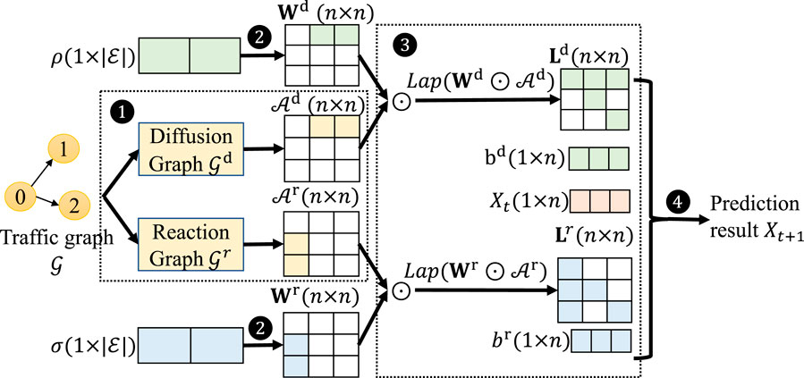
Figure 2. Reaction-Diffusion Graph Convolutional Network architecture for graph with $|\mathcal{V}|=3$ and $|\mathcal{E}|=2$. ❶ derives the diffusion and reaction adjacency matrices A^d and A^r; ❷ defines model weights ρ and σ for the reaction and diffusion networks and maps them to W^d and W^r with weights ρ and σ; ❸ characterizes the Laplacian graph L^d and L^r; ❹ defines the network prediction function.

Step 1: Define reaction and diffusion parameters. We define a diffusion graph ${\mathcal{G}}^d=(\mathcal{V},{\mathcal{E}}^d)$ and a reaction graph ${\mathcal{G}}^r=(\mathcal{V},{\mathcal{E}}^r)$ derived from the physical graph $\mathcal{G}$ (see ❶ in Figure 2). The diffusion graph represents whether two vertices are direct neighbors in the road direction—that is, ${\mathcal{E}}^d=\mathcal{E}$—and ${\mathcal{A}}^d=\mathcal{A}$; the reaction graph represents whether two vertices are direct neighbors in the opposite direction of a road segment—that is, ${\mathcal{E}}^r=\{(i,j):(j,i)\in \mathcal{E}\}$—and ${\mathcal{A}}^r={\mathcal{A}}^{\top }$, where ⊤ denotes matrix transpose. Define $\rho =\{{\rho }_{(i,j)}\in \mathbb{R}|(i,j)\in {\mathcal{E}}^d\}$, $\sigma =\{{\sigma }_{(i,j)}\in \mathbb{R}|(i,j)\in {\mathcal{E}}^r\}$, $b^d\in {\mathbb{R}}^n$, $b^r\in {\mathbb{R}}^n$ (see ❷ in Figure 2). Each parameter ρ_(i,j) (resp. σ_(i,j)) is a diffusion weight (resp. reaction weight) for edge (i, j). Each parameter in ρ and σ corresponds to a directed edge (i, j) in ${\mathcal{E}}^d$ and ${\mathcal{E}}^r$, respectively. ${\mathbf{W}}^d\in {\mathbb{R}}^{n\times n}$ is a sparse weight matrix for the diffusion graph ${\mathcal{G}}^d$, where ${\mathbf{W}}_{i,j}^d={\rho }_{(i,j)},\forall (i,j)\in {\mathcal{E}}^d$, otherwise ${\mathbf{W}}_{i,j}^d=0$. W^r for reaction graph ${\mathcal{G}}^r$ is defined in similarly, but the non-zero element at $(i,j)\in {\mathcal{E}}^r$ is σ_(i,j).

Step 2: Construct an RD feature encoding function. Let L^d (resp. L^r) be the corresponding Laplacian of the combination of diffusion (resp. reaction) weight tensor W^d (resp. W^r) and diffusion (resp. reaction) adjacency matrices ${\mathcal{A}}^d$ (resp. ${\mathcal{A}}^r$), then

$\begin{array}{cc}\hfill {\left({\mathbf{L}}^{d}X\left(t\right)\right)}_i& ={\displaystyle \sum _{\left(i,j\right)\in {\mathcal{E}}^d}}{\left({\mathbf{W}}^d\odot {\mathcal{A}}^d\right)}_{i,j}\left(X_j\left(t\right)-X_i\left(t\right)\right)\hfill \\ \hfill & ={\left(\left(Degree\left({\mathbf{W}}^d\odot {\mathcal{A}}^d\right)-{\mathbf{W}}^d\odot {\mathcal{A}}^d\right)X\left(t\right)\right)}_i,\hfill \end{array}$

where ⊙ denotes the Hadamard product, Degree (∗) is to calculate the degree matrix of an input adjacency matrix, and ${({\mathbf{L}}^r{X}_t)}_i$ represents a similar reaction process, but the weight tensor is W^r and adjacency matrix is ${\mathcal{A}}^r$. Specifically, the reaction and diffusion Laplacian L^r and L^d is the RD-informed feature encoding function O extracting speed differences between neighboring vertices (see ❸ in Figure 2).

Step 3: Using Eq. 4, we can define a prediction:

$\widehat{X}\left(t+1\right)=X\left(t\right)+\left({\mathbf{L}}^{d}X\left(t\right)+b^d\right)+\tanh \left({\mathbf{L}}^{r}X\left(t\right)+b^r\right),$

where L^d and L^r are the reaction and diffusion functions constructed earlier, corresponding to the function F = (L^dX_t + b^d) + tanh (L^rX_t + b^r) predicting the traffic speed using the reaction parameters ρ and the diffusion parameters σ (see ❹ in Figure 2).

6.2 Susceptible–infected–recovered (SIR)-GCN for infectious disease prediction

The SIR model is a typical model describing the temporal dynamics of an infectious disease by dividing the population into three categories: susceptible to the disease, infectious, and recovered with immunity. The SIR model is widely used in the study of diseases such as influenza and COVID (Cooper et al., 2020). Our approach is based on the SIR-Network Model proposed to model the spread of dengue fever (Stolerman et al., 2015), which we describe as follows. Let S_i(t), I_i(t), and R_i(t) denote the number of susceptible, infectious, and recovered at vertex $i\in \mathcal{V}$ at time t, respectively, and the total population at vertex i is assumed to be a constant—N_i = S_i(t) + I_i(t) + R_i(t).

The spread of infection between vertices is modeled using sparse travel matrices Φ ∈ [0,1]^n×n as ${\varphi }_{(i,j)},\forall (i,j)\in {\mathcal{E}}^d$; otherwise ϕ_(i,j) = 0, where ϕ_(i,j) ∈ [0, 1] is a parameter representing the fraction of resident population traveling from i to j; therefore, we require the fractions satisfy ${\sum }_{j=1}^n{\varphi }_{(i,j)}=1,\forall i\in \mathcal{V}$. The SIR-network model at vertex i is defined as

$\begin{array}{cc}\hfill \frac{d{S}_i\left(t\right)}{dt}=& -{\displaystyle \sum _{j=1}^n}{\displaystyle \sum _{k=1}^n}{\beta }_j{\varphi }_{\left(i,j\right)}{S}_i\left(t\right)\frac{{\varphi }_{\left(k,j\right)}{I}_k\left(t\right)}{N_j^p},\hfill \\ \hfill \frac{d{I}_i\left(t\right)}{dt}=& {\displaystyle \sum _{j=1}^n}{\displaystyle \sum _{k=1}^n}{\beta }_j{\varphi }_{\left(i,j\right)}{S}_i\left(t\right)\frac{{\varphi }_{\left(k,j\right)}{I}_k\left(t\right)}{N_j^p}-\gamma I_i,\hfill \\ \hfill \frac{d{R}_i\left(t\right)}{dt}=& \gamma I_i\left(t\right),\hfill \end{array}$

where β_i is the infection rate at vertex i, representing the probability that a susceptible population is infected at vertex i, γ is the recovery rate, representing the probability that an infected population is recovered, and $N_i^p={\sum }_{j=1}^n{\varphi }_{(j,i)}{N}_j$ is the total population traveling from all vertices to vertex i. We assume the recovery rates at all vertices are the same.

Step 1: Derive the susceptible and recovered numbers and define the travel matrices. We first define parameter β ∈ [0,1]ⁿ (n is the number of vertices) representing the infection rate, and parameter γ ∈ [0, 1] representing the recovered rate. Since the total population at vertex i is assumed to be a constant, the network level recovered and susceptible number is

$\begin{array}{cc}\hfill R\left(t\right)& =\gamma {\int }_{t_0}^{t}I\left(\tau \right)d\tau =\gamma {\displaystyle \sum _{{\tau =t}_0}^t}I\left(\tau \right)\Delta \tau ,\hfill \\ \hfill S\left(t\right)& =N-I\left(t\right)-R\left(t\right),\hfill \end{array}$

where dτ is the time interval for each sample, which we set to 1, N is the total number of the population of each state/prefecture, and t₀ is the starting time of the current epidemic (see ❶ in Figure 3). Next, the travel graph $\mathcal{G}$ is derived from the transportation data—that is, if there are flights between states/prefectures i and j—Φ_i,j = 1; otherwise ϕ_(i,j) = 0 (see ❷ in Figure 3).

Figure 3

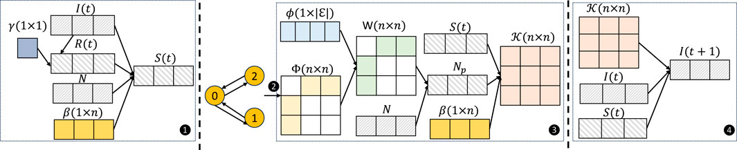
Figure 3. Susceptible-infected-recovered-GCN architecture for graph with $|\mathcal{V}|=3$ and $|\mathcal{E}|=2$. ❶ derives the susceptible and recovered numbers; ❷ defines travel matrices using the transportation data; ❸ characterizes the transformation matrix $\mathcal{K}$ using Eq. 9; ❹ defines the network prediction function using Eq. 10.

Step 2: Construct the SIR function. Define $\varphi =\{{\varphi }_{(i,j)}\in \mathbb{R}|{\mathrm{\Phi }}_{i,j}>0\}$. Each ϕ represents the fraction of population traveling from i to j, as defined earlier. $\mathbf{W}\in {\mathbb{R}}^{n\times n}$ is a sparse weight matrix for the travel graph, where W_i,j = ϕ_(i,j), ∀Φ_i,j > 0; otherwise W = 0. Then, the differential equation system (20) is equivalent to:

$\frac{dI\left(t\right)}{dt}=\left(\mathcal{K}-\gamma \right)I\left(t\right),(8)$

where I(t) is the feature (X(t) mentioned earlier) representing the number of infectious people. Then, the transformation matrix $\mathcal{K}$ connecting I(t) and I (t + 1) at neighboring time is

${\mathcal{K}}_{i,j}={\displaystyle \sum _{j=1}^n}{\beta }_j{\mathbf{W}}_{i,j}{\mathbf{W}}_{k,j}\frac{S_i}{N_j^p},(9)$

The dynamics-informed feature encoding function O is utilized to approximate the counts of susceptible and recovered populations and to estimate the infectious people likely to travel, approximated by the transportation data (see ❸ in Figure 3).

Step 3: Using Eq. 4 and 8, 9, the prediction is defined as:

$\widehat{I}\left(t+1\right)=I\left(t\right)+\left(\mathcal{K}-\gamma \right)I\left(t\right),(10)$

(see ❹ in Figure 3).

7 Evaluation

In this section, we compare the performance of these domain-ODE-informed GCNs with baselines when tested with mismatched data and demonstrate that our approach is more robust to such mismatched scenarios.

7.1 Experiment settings

7.1.1 Datasets

Our experiments are conducted on three real-world datasets (Metra-la, Pems-bay, and Seattle-loop) for traffic prediction and on two real-world datasets (in Japan and US) for disease prediction. The details are shown in Table 1.

Table 1

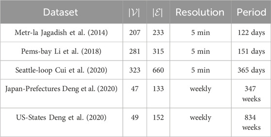
Table 1. Dataset description.

7.1.2 Evaluation metric

The loss function we use is the mean absolute error and the root mean squared error: $MAE(X(t),\widehat{X}(t))=\frac{1}{n}{\sum }_{i=1}^n|x_i(t)-{\widehat{x}}_i(t)|$, $RMSE(X(t),\widehat{X}(t))={\left.{(\frac{1}{n}{\sum }_{i=1}^n(x_i(t)-{\widehat{x}}_i(t)))}^2\right)}^{\frac{1}{2}}$. We also use MAE and RMSE to evaluate models.

7.1.3 Baselines

For traffic prediction tasks, we compare RDGCN with STGCN (Yu et al., 2018), MTGNN (Wu et al., 2020), GTS (Shang et al., 2021), STGNCDE (Choi et al., 2022), and MTGODE (Jin et al., 2022). They are influential and the best-performing deep learning models for predicting traffic speed using historical speed alone. We also use Model-Agnostic Meta-Learning (MAML) (Finn et al., 2017) to help baseline models, and our approach adapts quickly to tasks using good initial weights generated by MAML. For disease prediction, we compare SIRGCN with two state-of-the-art models for infection prediction: ColaGNN (Deng et al., 2020) and EpiGNN (Xie et al., 2023).

7.1.4 Evaluation

We assume that all zeros in the datasets are missing values, and we remove the predicted speed when the ground truth is 0, or when the last speed recorded is 0.

7.1.5 Hyperparameter settings

RDGCN and SIRGCN are optimized via Adam. The batch size is set as 64. The learning rate is set as 0.001, and the early stopping strategy is used with a patience of 30 epochs. These settings are the same as those used in baseline models to set up a fair comparison. In traffic speed prediction, the training and validation sets are split by a ratio of 3:1 from the weekday subset, and the test data are sampled from the weekend subset with different patterns. As for baselines, we use identical hyperparameters as released in their works. In ILI prediction, the training and validation set are split by a ratio of 5:2 from the winter–summer subset, and the test data are sampled from the spring–fall subset with different patterns. The susceptible population at the beginning of each ILI period is 10% of the total population in each prefecture or state. As for baselines, we also use identical hyperparameters as released in their works. We approximate the total number of populations by the average of the annual sum of infectious cases multiplied by 10. In contrast to black-box baseline models, our model is domain-ODE-informed, and the architecture is determined by the physical network and the domain differential equations.

7.1.6 MAML settings

Our experiment involved the following steps. 1) We randomly selected sequences of 12 consecutive weekdays (the same as in the limited and mismatched data experiment), and sampled 4-h data as the training set. We evaluated the model with hourly data on weekends. 2) We divided the training set into two equal parts: the support set and the query set. 3) We used the support set to compute adapted parameters. 4) We used the adapted parameters to update the MAML parameters on the query set. 5) We repeated this process 200 times to obtain initial parameters for the baseline model. 6) We trained baselines using the obtained initial parameters. The learning rate for the inner loop was 0.00005, and for the outer loop was 0.0005, and MAML was trained for 200 epochs.

7.2 Results and analysis

7.2.1 Mismatched data experiments for RDGCN

We first explore the performance of the models when they are trained using mismatched data from certain conditions and tested using alternate, mismatched conditions. Specifically, the models were trained for 4-h data on weekdays (e.g., 8:00–12:00 on weekdays) and selected and evaluated with hourly data on weekends (e.g., 13:00–14:00 on weekends). In limited data and mismatched conditions (Figure 4A), the training set consists of data from five different sequences of 12 consecutive weekdays selected randomly from the available data. This experiment aims to replicate scenarios where data collection is challenging, and traffic patterns undergo rapid changes. In mismatched conditions without data limitations (Figure 4B), the training set consists of data from all available weekdays. This captures instances where data collection is comparatively less arduous, although the traffic pattern retains the potential to shift swiftly. The results are shown in Figure 4, where each curve denotes the average test prediction MAE and RMSE of models. In Figure 4A, we compare the performance of our approach with that of the STGCN, MTGNN, GTS, MTGODE, STGNCDE, and RDGCN in the mismatched data, when the training process is augmented with MAML. Figure 4B plots the prediction MAE and RMSE of baseline models and RDGCN over time, given all available weekday data. Corresponding numerical results is shown in Table 2.

Figure 4

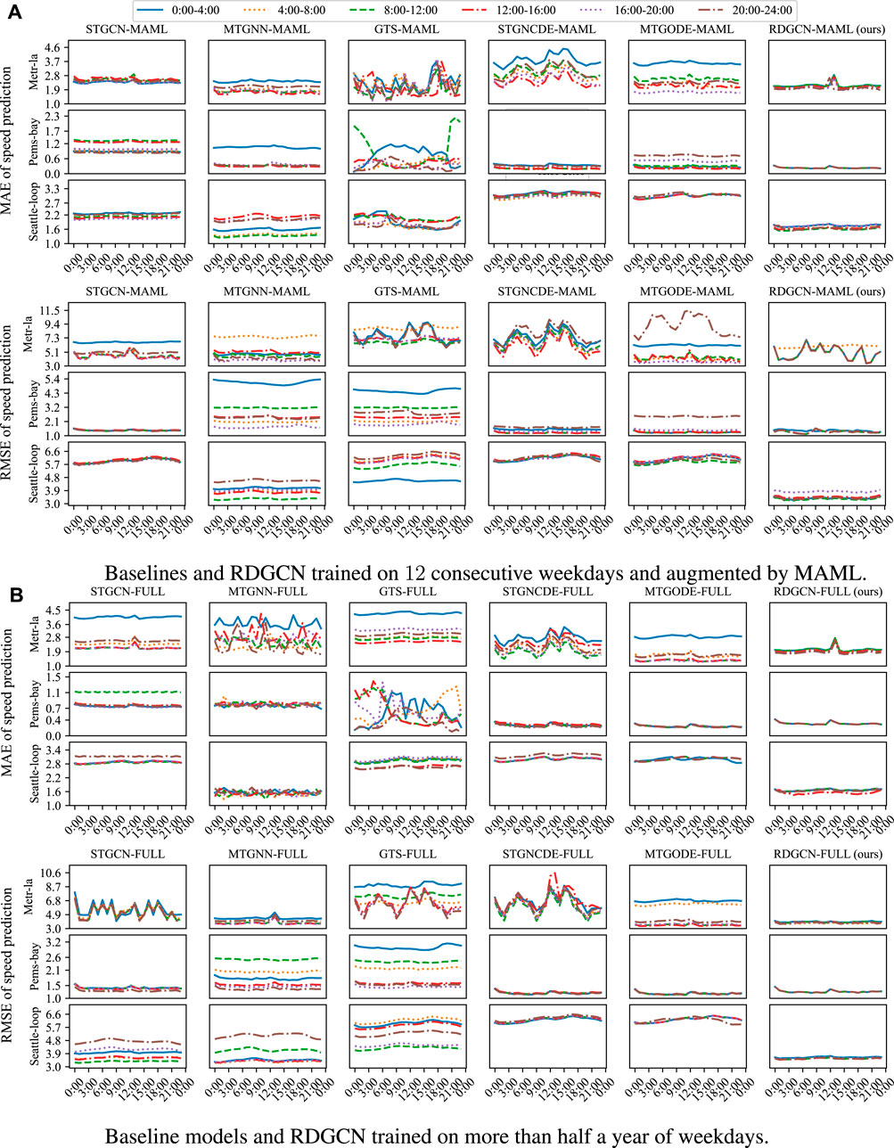
Figure 4. (A) The results of RDGCN are very close regardless of the period of the training set. (B) Even though all the models are trained using all available weekdays, the results of RDGCN are still closer, regardless of the period, than baseline models.

Table 2

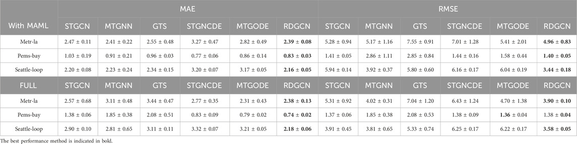
Table 2. Numerical result of Figure 4: the mean and STD of prediction MAE, RMSE of RDGCN, and baselines on three real-world datasets.

In Figure 4, all RDGCN models have nearly identical performance regardless of which time window of data is used for training. The MAE of all the RDGCN models is uniformly low (i.e., small y-axis values), and there is very low variance in performance across RDGCN models trained with different time windows (i.e., the curves of average MAE is close to the curves of maximum MAE). However, the performance of baseline models is significantly different depending on the training set, and some can have a relatively high MAE (e.g., the curve of STGCN on the Pems-bay dataset has much higher MAE values than that for RDGCN over time). From Figure 4B, we can see that even when the model is trained using all available weekday data, RDGCN outperforms the baseline models where the variance is across time, and across models is very low. While more data bring some gain to baseline models, its impact on RDGCN is fairly limited, indicating that RDGCN performs well in different testing domains without needing additional training data. In Table 2, RDGCN has lower MAE and lower RMSE loss with less variance, which further supports the observation in Figure 4. We admit that MTGODE also works well in Pems-bay when full data are used for training, but the superiority is not significant.

These test results support our hypothesis that incorporating traffic dynamics into the learning model makes it more robust to this kind of domain generalization (data from mismatched training and testing conditions). We speculate that this is a consequence of our model capturing the relative changes in speed through the dynamical equations, whereas existing baseline models are black-box models that derive complex functions of the absolute speed values across time. In effect, when there is a mismatch, the underlying nature of traffic dynamics is less likely to be impacted, whereas the complex patterns of absolute speed values might vary significantly across domains. This is particularly true when dealing with limited data that do not contain all possible patterns. At the same time, RDGCN is designed to make predictions based on neighboring vertices, so even if the speed patterns of a distant sensor and a close sensor are similar (e.g., both are free flow), the model uses close sensors to make predictions. We note that the prediction of RDGCN is not uniformly better than that of baselines (e.g., the prediction of MTGNN trained by Seattle weekday data from 8:00 to 12:00 is better than the prediction of RDGCN), and one possible reason is that speed pattern mismatches between weekdays and weekends are not always significant (e.g., when the training weekday is a holiday). Furthermore, the predictions of MTGNN and MTGODE exhibit a slight superiority over RDGCN in the Metr-la dataset in certain windows. Our conjecture is that the mix-hop layers enable these models to assign higher significance to learn short-term patterns, which likely does not change much between the training and test data. We acknowledge that RDGCN is not always better than baselines under RMSE, as when STGCN is trained with weekday data from 16:00–20:00 in Metr-la. One possible reason is that the mismatches between the training and test data are not significant during the corresponding time period. The prediction results of RDGCN in terms of RMSE may not always be stable. For instance, when considering the models for the 4:00–8:00 time period in Metr-la, we observe distinct prediction outcomes. This variation could be due to the difference between the pattern of the morning rush hour during selected weekdays and the pattern during weekends. When the training set includes all available weekday data, the predictions of RDGCN demonstrate stability. Although real-world data under situations such as disasters are hard to obtain, our approach of splitting the dataset emulates test scenarios that are sufficiently different from the training dataset to demonstrate the robustness of our approach.

7.2.2 Mismatched data experiments for SIRGCN

We explored the performance of SIRGCN under mismatched situations. Since infection spread and travel patterns vary from season to season, we trained our model and the baseline models with ILI data recorded in summer and winter and tested the predictions on data in spring and fall. The result is shown in Table 3, where each element denotes the MAE and RMSE under different seasons.

Table 3

Table 3. Evaluation of models under mismatched data.

The results demonstrate that SIRGCN performs consistently better under the mismatched data scenario with low MAE and RMSE than the baseline models. Although SIRGCN does not significantly outperform the deep-learning-based ColaGNN model, we note that SIRGCN makes predictions using only the latest observation at one time point augmented by approximating the total susceptible and recovered populations, as specified by the domain equations, whereas the baselines which consider the disease propagation as a black-box model require more than 7 years data to train and 20 weeks-worth of data to make their predictions.

The two datasets are used for testing, but the theory can also apply to other applications, such as air quality forecasting and molecular simulation, where there are underlying graphical models and the ODE domain is well developed. Overall, these evaluations validate the main hypothesis of this paper wherein integrating domain differential equations into GCN allows for better robustness.

8 Ablation study

8.1 Analysis of RDGCN in traffic speed prediction

8.1.1 Are reaction and diffusion processes essential?

In this section, we investigate the prediction models that incorporate the reaction and the diffusion equations independently under limited and mismatched data to understand whether both the reaction and diffusion processes are essential. We use the same training set (i.e., 12 consecutive working days selected randomly) and test set (i.e., hourly weekend data) as Section 7.2. The curves of MAE versus time using the model incorporating the reaction equation, the diffusion equation, and the reaction-diffusion equation are shown in Figure 5A, and the corresponding curves of RMSE versus time are shown in Figure 5B.

Figure 5

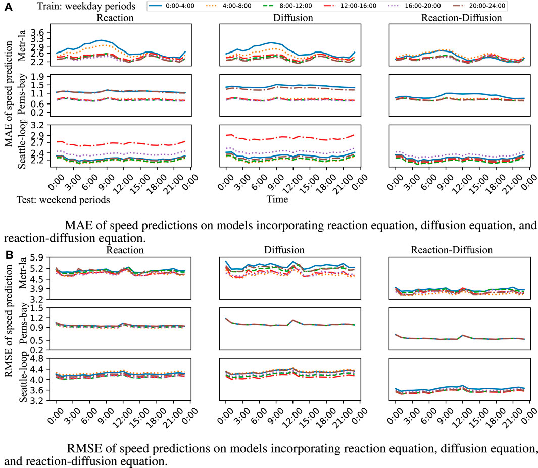
Figure 5. The predictions of the reaction–diffusion model, employing both MAE and RMSE loss, exhibit lower prediction error, whereas the predictions of only the reaction models or only the diffusion models demonstrate weaker performance in at least one time period. (A) MAE of speed predictions on models incorporating reaction equation, diffusion equation, and reaction-diffusion equation. (B) RMSE of speed predictions on models incorporating reaction equation, diffusion equation, and reaction-diffusion equation.

Figure 5 indicates that the predictions of all models with the reaction–diffusion equation provide low MAE/RMSE with low variance (i.e., the difference between curves with the highest and lowest MAE/RMSE is small) over time. However, the predictions of the reaction models only and the diffusion models only have weaker performance in at least one time period. We speculate that using only the reaction equation or the diffusion equation is not sufficient to completely capture the dynamics of the traffic speed change. Furthermore, the prediction of the model incorporating the reaction–diffusion equation is not uniformly better than the prediction of the model incorporating only the reaction or diffusion equation. One possible reason is that the reaction or diffusion processes do not always exist in a specific period (e.g., if two neighboring road segments are in free-flow during the test period, the traffic speeds at the two segments do not affect each other. Thus, there is neither diffusion nor reaction between these two road segments). These observations further strengthen that both the reaction and diffusion processes are necessary for a reliable prediction.

8.1.2 Impact of data volume

We further investigate the influence of training data volume on the performance of baseline models and RDGCN under a mismatched setting. We focus on assessing the adequacy of training data for both morning (8:00–12:00) and evening rush hour (16:00–20:00) scenarios using the Metr-la dataset. These periods exhibit considerable patterns and exhibit relatively minor mismatches between the training and test datasets. To this end, we randomly select contiguous weekdays ranging from 20% to the entire dataset for training the models. The MAE of speed prediction across varying quantities of training data is shown in Figure 6.

Figure 6

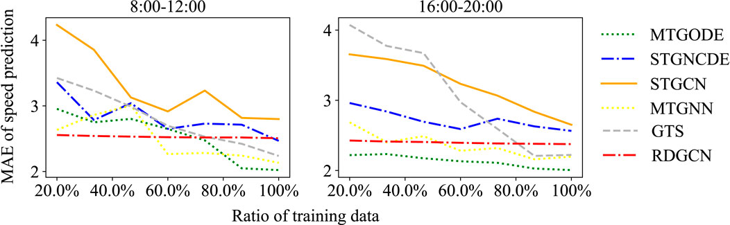
Figure 6. Feeding more training data does not lead to a significant change in the MAE of RDGCN’s prediction.

Figure 6 showcases the performance characteristics of the RDGCN and baseline models over the specified time intervals. Remarkably, the performance of RDGCN remains consistent irrespective of the training dataset size. Conversely, the predictive capabilities of STGNCDE and MTGODE are notably contingent upon the amount of training data employed. The observed trend underscores increased training data volume and directly correlates with enhanced prediction accuracy. In the morning rush hour, MTGODE achieves optimal performance with approximately 75% of training data (equivalent to 60 weekdays), while STGNCDE demonstrates comparable performance when trained on the entire weekday dataset. We note that the superiority of RDGCN over baseline models is not universally consistent, as elucidated earlier. Notably, integrating domain differential equations drastically reduces the size of the hypothesis class, thereby filtering out erroneous hypotheses often prevalent in conventional black-box graph learning models. Consequently, domain-differential-equation-informed GCNs exhibit remarkable robustness on relatively smaller training datasets.

8.2 Analysis of SIRGCN in ILI prediction

8.2.1 Do the infection rates vary among different vertices?

In this section, we delve into the question of whether we require an individual infection rate for each vertex in ILI prediction. We specifically examine two approaches: one where we assign a unique infection rate, denoted β_i, to each vertex i, resulting in a SIRGCN with n infection rates (SIRGCN-n), and another approach where we assign a single infection rate, denoted β, to all vertices (SIRGCN-1). We report the MAE and RMSE of the prediction under mismatched data (trained using winter–summer data and test using spring–fall data) in Table 4.

Table 4

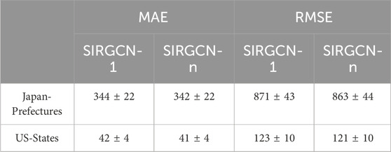
Table 4. Evaluation of models under mismatched data.

Table 4 shows that employing multiple infection rates leads to more accurate predictions, particularly in the case of the US-state dataset. By assigning individual infection rates to each vertex, we achieve a reduction of 2.4% in MAE (and 1.6% in RMSE). However, the advantage of utilizing multiple infection rates is less pronounced $(<1\%)$ in the ILI prediction of Japan. There could be two potential explanations for this. First, the size of prefectures in Japan is not as substantial as that of the states in the United States. Second, climates across Japan are relatively homogeneous, whereas climates across different US states exhibit significant variations, such as wet coastal and dry inland areas.

8.2.2 Predictions in different seasons

Learning patterns across different trends become challenging when baseline models are not trained using the same trend. For example, during winter the infectious number shows an increasing trend, whereas during spring it exhibits a decreasing trend. Figure 7 shows the predicted number of infectious cases alongside the ground truth data, revealing that SIRGCN’s prediction aligns better with the ground truth. Conversely, EpiGNN’s prediction performs poorly during the decline phase and when the number of infections approaches 0.

Figure 7

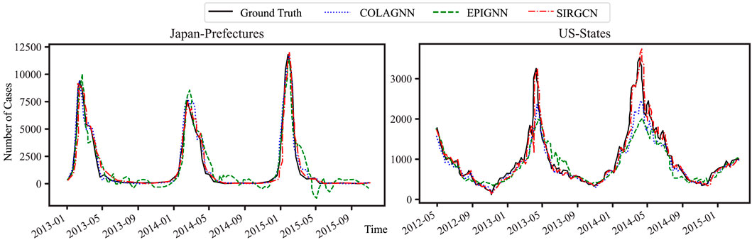
Figure 7. SIRGCN can make accurate predictions in the decreasing phase, while EpiGNN makes bad predictions in the corresponding phase.

In the case of US-state ILI prediction in May 2014, both COLAGNN and EPIGNN fail to make accurate predictions around the peak, while SIRGCN demonstrates its effectiveness during the corresponding period with the help of the SIR-network model.

9 Model efficiency in computation time

The training and inference times (on two NVIDIA-2080ti graphic cards) of STGCN, MTGNN, GTS, STGNCDE, STGODE, and RDGCN on the Metr-la dataset are demonstrated in Table 5. It is observed that RDGCN takes less time in both training and inference than the other models. This efficiency can be attributed to RDGCN’s significantly fewer parameters in contrast to the baseline models. While the spatial convolutional layers exhibit similar complexities across all baseline models, the baseline models use richer temporal layers containing tens of thousands of parameters. In a traffic network where the number of edges is only slightly greater than the number of vertices, the parameter count of RDGCN $(2|\mathcal{V}|+2|\mathcal{E}|)$ closely resembles that of two GCN layers in baseline models, thereby saving parameters from complex temporal convolutional layers. Similarly, in the disease propagation network, SIRGCN’s parameter count $(|\mathcal{V}|+|\mathcal{E}|+1)$ is lower than that of baseline models. Thus, the proposed methods require less training data, computation resources, and time, making them easier to train than baseline models.

Table 5

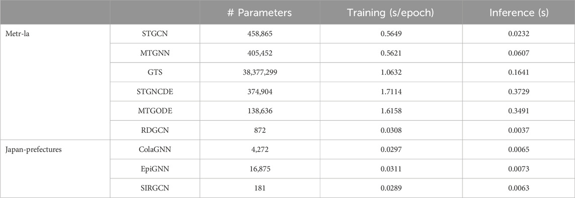
Table 5. Computation time on Metr-la dataset.

The training and inference time of ColaGNN, EpiGNN, and SIRGCN are shown in Table 5. SIRGCN has significantly fewer parameters than the baseline models. We acknowledge that the computational time of SIRGCN is similar to that of the baseline models, as the baselines are not as deep or dense as traffic prediction models and do not require a large amount of data for training.

10 Conclusion

In this paper, we investigate the challenging problem of graph time-series prediction when training and test data are drawn from different or mismatched scenarios. To address this challenge, we propose a methodological approach to integrate domain differential equations in graph convolutional networks to capture the common data behavior across data distributions. We theoretically justify the robustness of this approach under certain conditions on the underlying domain and data. By operationalizing our approach, we propose two novel dynamics-informed GCNs: RDGCN and SIRGCN. These architectures fuse traffic speed reaction-diffusion equations and susceptible-infected-recovered infectious disease spread equations, respectively. Through rigorous numerical evaluation, we demonstrate the robustness of our models in mismatched data scenarios. Both models can significantly reduce the number of parameters while maintaining prediction accuracy and robustness, thus requiring less training data and shorter training time. The findings showcased in this study underscore the transformative potential of domain-ODE-informed models as a burgeoning category within the domain of graph neural networks. This framework can pave the way for future exploration addressing the challenges of domain generalization in other contexts.

Data availability statement

The original contributions presented in the study are included in the article/Supplementary Material; further inquiries can be directed to the corresponding author.

Author contributions

YS: conceptualization, data curation, formal analysis, investigation, methodology, software, validation, visualization, writing–original draft, and writing–review and editing. CC: investigation, visualization, and writing–review and editing. YX: investigation, visualization, and writing–review and editing. SX: conceptualization, funding acquisition, investigation, supervision, and writing–review and editing. RB: conceptualization, funding acquisition, investigation, supervision, and writing–review and editing. PV: conceptualization, funding acquisition, investigation, project administration, resources, supervision, and writing–review and editing.

Funding

The author(s) declare that financial support was received for the research, authorship, and/or publication of this article. This work was partly funded through a Lehigh internal Accelerator Grant, Grants CCF-1617889 and IIS-1909879 from the National Science Foundation and the U.S. Office of Naval Research under Grant N00014-22-1-2626. SX was partly supported by the Education Bureau of Guangzhou Municipality and the Guangzhou-HKUST (GZ) Joint Funding Program (Grant 583 No. 2023A03J0008).

Conflict of interest

The authors declare that the research was conducted in the absence of any commercial or financial relationships that could be construed as a potential conflict of interest.

Publisher’s note

All claims expressed in this article are solely those of the authors and do not necessarily represent those of their affiliated organizations, or those of the publisher, the editors, and the reviewers. Any product that may be evaluated in this article, or claim that may be made by its manufacturer, is not guaranteed or endorsed by the publisher.

Supplementary material

The Supplementary Material for this article can be found online at: https://www.frontiersin.org/articles/10.3389/fmech.2024.1397131/full#supplementary-material

Footnotes

¹E.g., congestion is caused by the increasing traffic demand.

²E.g., temporary change of travel demand.

³In the Supplementary Appendix, we show that the datasets used satisfy these assumptions.

⁴E.g., consider the evolution of traffic speed: during morning rush hour, training data reflect significant traffic demand influencing speed, whereas test data from midnight reflect negligible traffic demand, and thus no speed change.

⁵E.g., during the morning rush hour, a two-hop neighbor facilitates positive speed changes for the target. However, as the evening rush hour ensues, the same two-hop neighbor can result in negative speed changes due to shifts in population flow, with cars redirecting to different vertices at night.

References

Asikis, T., Böttcher, L., and Antulov-Fantulin, N. (2022). Neural ordinary differential equation control of dynamics on graphs. Phys. Rev. Res. 4, 013221. doi:10.1103/physrevresearch.4.013221

CrossRef Full Text | Google Scholar

Bellocchi, L., and Geroliminis, N. (2020). Unraveling reaction-diffusion-like dynamics in urban congestion propagation: insights from a large-scale road network. Sci. Rep. 10, 4876. doi:10.1038/s41598-020-61486-1

PubMed Abstract | CrossRef Full Text | Google Scholar

Bui, K.-H. N., Cho, J., and Yi, H. (2022). Spatial-temporal graph neural network for traffic forecasting: an overview and open research issues. Appl. Intell. 52, 2763–2774. doi:10.1007/s10489-021-02587-w

CrossRef Full Text | Google Scholar

Chen, C., Hu, J., Meng, Q., and Zhang, Y. (2011). “Short-time traffic flow prediction with arima-garch model,” in 2011 IEEE Intelligent Vehicles Symposium (IV) (IEEE), Baden-Baden, Germany, June, 2011, 607–612.

CrossRef Full Text | Google Scholar

Chen, R. T., Rubanova, Y., Bettencourt, J., and Duvenaud, D. K. (2018). Neural ordinary differential equations. Adv. neural Inf. Process. Syst. 31.

Google Scholar

Choi, J., Choi, H., Hwang, J., and Park, N. (2022). Graph neural controlled differential equations for traffic forecasting. Proc. AAAI Conf. Artif. Intell. 36, 6367–6374. doi:10.1609/aaai.v36i6.20587

CrossRef Full Text | Google Scholar

Cooper, I., Mondal, A., and Antonopoulos, C. G. (2020). A sir model assumption for the spread of covid-19 in different communities. Chaos, Solit. Fractals 139, 110057. doi:10.1016/j.chaos.2020.110057

PubMed Abstract | CrossRef Full Text | Google Scholar

Cui, Z., Ke, R., Pu, Z., Ma, X., and Wang, Y. (2020). Learning traffic as a graph: a gated graph wavelet recurrent neural network for network-scale traffic prediction. Transp. Res. Part C Emerg. Technol. 115, 102620. doi:10.1016/j.trc.2020.102620

CrossRef Full Text | Google Scholar

Deng, S., Wang, S., Rangwala, H., Wang, L., and Ning, Y. (2020). “Cola-gnn: cross-location attention based graph neural networks for long-term ili prediction,” in CIKM, Virtual Event, October 2020.

CrossRef Full Text | Google Scholar

Fan, X., Wang, Q., Ke, J., Yang, F., Gong, B., and Zhou, M. (2021). “Adversarially adaptive normalization for single domain generalization,” in CVPR, Nashville, TN, USA, June, 2021.

CrossRef Full Text | Google Scholar

Finn, C., Abbeel, P., and Levine, S. (2017). “Model-agnostic meta-learning for fast adaptation of deep networks,” in ICML, Sydney, Australia, August, 2017.

Google Scholar

Guo, S., Lin, Y., Feng, N., Song, C., and Wan, H. (2019). Attention based spatial-temporal graph convolutional networks for traffic flow forecasting. AAAI 33, 922–929. doi:10.1609/aaai.v33i01.3301922

CrossRef Full Text | Google Scholar

Han, L., Du, B., Sun, L., Fu, Y., Lv, Y., and Xiong, H. (2021). “Dynamic and multi-faceted spatio-temporal deep learning for traffic speed forecasting,” in SIGKDD, Virtual Event Singapore, August, 2021.

CrossRef Full Text | Google Scholar

Huang, J., and Agarwal, S. (2020). “Physics informed deep learning for traffic state estimation,” in 2020 IEEE 23rd International Conference on Intelligent Transportation Systems (ITSC), Rhodes, Greece, September, 2020, 1–6.

CrossRef Full Text | Google Scholar

Jagadish, H. V., Gehrke, J., Labrinidis, A., Papakonstantinou, Y., Patel, J. M., Ramakrishnan, R., et al. (2014). Big data and its technical challenges. Commun. ACM 57, 86–94. doi:10.1145/2611567

CrossRef Full Text | Google Scholar

Jayatilaka, G., Hassan, J., Marikkar, U., Perera, R., Sritharan, S., Weligampola, H., et al. (2020). Use of artificial intelligence on spatio-temporal data to generate insights during covid-19 pandemic: a review. Available at: https://www.medrxiv.org/content/10.1101/2020.11.22.20232959v5.

Google Scholar

Ji, J., Wang, J., Jiang, Z., Jiang, J., and Zhang, H. (2022). Stden: towards physics-guided neural networks for traffic flow prediction. Proc. AAAI Conf. Artif. Intell. 36, 4048–4056. doi:10.1609/aaai.v36i4.20322

CrossRef Full Text | Google Scholar

Jia, J., and Benson, A. R. (2019). Neural jump stochastic differential equations. Adv. Neural Inf. Process. Syst. 32.

Google Scholar

Jin, M., Zheng, Y., Li, Y.-F., Chen, S., Yang, B., and Pan, S. (2022). Multivariate time series forecasting with dynamic graph neural odes. IEEE Trans. Knowl. Data Eng. 35, 9168–9180. doi:10.1109/tkde.2022.3221989

CrossRef Full Text | Google Scholar

Karniadakis, G. E., Kevrekidis, I. G., Lu, L., Perdikaris, P., Wang, S., and Yang, L. (2021). Physics-informed machine learning. Nat. Rev. Phys. 3, 422–440. doi:10.1038/s42254-021-00314-5

CrossRef Full Text | Google Scholar

Kessels, F., and Kessels, R. (2019). Traffic flow modelling. Berlin, Germany: Springer.

Google Scholar

Kipf, T. N., and Welling, M. (2017). Semi-supervised classification with graph convolutional networks. ICLR.

Google Scholar

Kumar, S. V., and Vanajakshi, L. (2015). Short-term traffic flow prediction using seasonal arima model with limited input data. Eur. Transp. Res. Rev. 7, 21–29. doi:10.1007/s12544-015-0170-8

CrossRef Full Text | Google Scholar

Kuznetsov, V., and Mohri, M. (2016). “Time series prediction and online learning,” in COLT, New-York City, USA, June, 2016.

Google Scholar

Lakkaraju, H., Bach, S. H., and Leskovec, J. (2016). “Interpretable decision sets: a Joint framework for description and prediction,” in SIGKDD, San Francisco, USA, August, 2016, 1675–1684.

Google Scholar

Li, Y., Yu, R., Shahabi, C., and Liu, Y. (2018). “Diffusion convolutional recurrent neural network: data-driven traffic forecasting,” in ICLR, Vancouver Convention Center, Vancouver CANADA, May, 2018.

Google Scholar

Loder, A., Ambühl, L., Menendez, M., and Axhausen, K. W. (2019). Understanding traffic capacity of urban networks. Sci. Rep. 9, 16283–16310. doi:10.1038/s41598-019-51539-5

PubMed Abstract | CrossRef Full Text | Google Scholar

Longa, A., Lachi, V., Santin, G., Bianchini, M., Lepri, B., Lio, P., et al. (2023). Graph neural networks for temporal graphs: state of the art, open challenges, and opportunities. Available at: https://arxiv.org/abs/2302.01018.

Google Scholar

Lou, Y., Caruana, R., and Gehrke, J. (2012). “Intelligible models for classification and regression,” in SIGKDD, Beijing, China, August, 2012.

CrossRef Full Text | Google Scholar

Maier, A. K., Syben, C., Stimpel, B., Würfl, T., Hoffmann, M., Schebesch, F., et al. (2019). Learning with known operators reduces maximum error bounds. Nat. Mach. Intell. 1, 373–380. doi:10.1038/s42256-019-0077-5

PubMed Abstract | CrossRef Full Text | Google Scholar

Montes de Oca Zapiain, D., Stewart, J. A., and Dingreville, R. (2021). Accelerating phase-field-based microstructure evolution predictions via surrogate models trained by machine learning methods. npj Comput. Mater. 7 (3), 3. doi:10.1038/s41524-020-00471-8

CrossRef Full Text | Google Scholar

Morid, M. A., Sheng, O. R. L., and Dunbar, J. (2023). Time series prediction using deep learning methods in healthcare. ACM Trans. Manag. Inf. Syst. 14, 1–29. doi:10.1145/3531326

CrossRef Full Text | Google Scholar

Qiao, F., Zhao, L., and Peng, X. (2020). “Learning to learn single domain generalization,” in CVPR, Seattle, WA, United States, June, 2020.

CrossRef Full Text | Google Scholar

Raissi, M., Perdikaris, P., and Karniadakis, G. E. (2019). Physics-informed neural networks: a deep learning framework for solving forward and inverse problems involving nonlinear partial differential equations. J. Comput. Phys. 378, 686–707. doi:10.1016/j.jcp.2018.10.045

CrossRef Full Text | Google Scholar

Redko, I., Morvant, E., Habrard, A., Sebban, M., and Bennani, Y. (2020). A survey on domain adaptation theory: learning bounds and theoretical guarantees. Available at: https://arxiv.org/abs/2004.11829.

Google Scholar

Robey, A., Pappas, G. J., and Hassani, H. (2021). “Model-based domain generalization,” in Advances in Neural Information Processing Systems 34, 20210–20229.

Google Scholar

Scholz, G., and Scholz, F. (2015). First-order differential equations in chemistry. ChemTexts 1, 1–12. doi:10.1007/s40828-014-0001-x

CrossRef Full Text | Google Scholar

Shang, C., Chen, J., and Bi, J. (2021). “Discrete graph structure learning for forecasting multiple time series,” in ICLR, Virtual Only Conference, May, 2021.

Google Scholar

Stolerman, L. M., Coombs, D., and Boatto, S. (2015). Sir-network model and its application to dengue fever. SIAM J. Appl. Math. 75, 2581–2609. doi:10.1137/140996148

CrossRef Full Text | Google Scholar

Thodi, B. T., Khan, Z. S., Jabari, S. E., and Menéndez, M. (2022). Incorporating kinematic wave theory into a deep learning method for high-resolution traffic speed estimation. IEEE Trans. Intelligent Transp. Syst. 23, 17849–17862. doi:10.1109/tits.2022.3157439

CrossRef Full Text | Google Scholar

Van Der Voort, M., Dougherty, M., and Watson, S. (1996). Combining kohonen maps with arima time series models to forecast traffic flow. Transp. Res. Part C Emerg. Technol. 4, 307–318. doi:10.1016/s0968-090x(97)82903-8

CrossRef Full Text | Google Scholar

van Wageningen-Kessels, F., Van Lint, H., Vuik, K., and Hoogendoorn, S. (2015). Genealogy of traffic flow models. EURO J. Transp. Logist. 4, 445–473. doi:10.1007/s13676-014-0045-5

CrossRef Full Text | Google Scholar

Varshney, K. R. (2020). “On mismatched detection and safe, trustworthy machine learning,” in CISS, Princeton, NJ, USA, March, 2020.

CrossRef Full Text | Google Scholar

Veličković, P., Cucurull, G., Casanova, A., Romero, A., Lio, P., and Bengio, Y. (2018). “Graph attention networks,” in ICLR, Vancouver Convention Center, Vancouver CANADA, April, 2018.

Google Scholar

Wang, J., Lan, C., Liu, C., Ouyang, Y., Qin, T., Lu, W., et al. (2022). Generalizing to unseen domains: a survey on domain generalization. TKDE 35, 1. doi:10.1109/tkde.2022.3178128

CrossRef Full Text | Google Scholar

Wang, Z., Luo, Y., Qiu, R., Huang, Z., and Baktashmotlagh, M. (2021). “Learning to diversify for single domain generalization,” in ICCV, Montreal, Canada, October, 2021.

CrossRef Full Text | Google Scholar

Wu, Z., Pan, S., Long, G., Jiang, J., Chang, X., and Zhang, C. (2020). “Connecting the dots: multivariate time series forecasting with graph neural networks,” in SIGKDD, Virtual Conference, August, 2020.

CrossRef Full Text | Google Scholar

Xhonneux, L.-P., Qu, M., and Tang, J. (2020). “Continuous graph neural networks,” in ICML, Virtual Conference, July, 2020.

Google Scholar

Xian, X., Hong, M., and Ding, J. (2022). “Mismatched supervised learning,” in ICASSP, Singapore, May, 2022.

CrossRef Full Text | Google Scholar

Xie, F., Zhang, Z., Li, L., Zhou, B., and Tan, Y. (2023). “Epignn: exploring spatial transmission with graph neural network for regional epidemic forecasting,” in ECML PKDD, Torino, September, 2023, 469–485.

CrossRef Full Text | Google Scholar

Ying, R., Bourgeois, D., You, J., Zitnik, M., and Leskovec, J. (2019). Gnn explainer: a tool for post-hoc explanation of graph neural networks. Available at: https://arxiv.org/abs/1903.03894.

Google Scholar

Yu, B., Yin, H., and Zhu, Z. (2018). “Spatio-temporal graph convolutional networks: a deep learning framework for traffic forecasting,” in IJCAI, Stockholmsmässan, July, 2018.

CrossRef Full Text | Google Scholar

Zhou, K., Liu, Z., Qiao, Y., Xiang, T., and Loy, C. C. (2021). Domain generalization in vision: a survey. Available at: https://arxiv.org/abs/2103.02503.

Google Scholar

Zhou, K., Liu, Z., Qiao, Y., Xiang, T., and Loy, C. C. (2022). Domain generalization: a survey. IEEE Trans. Pattern Analysis Mach. Intell. 45, 4396–4415. doi:10.1109/tpami.2022.3195549

CrossRef Full Text | Google Scholar