Flow-based parameterization for DAG and feature discovery in scientific multimodal data

Representation learning algorithms are often used to extract essential features from high-dimensional datasets. These algorithms commonly assume that such features are independent. However, multimodal datasets containing complementary information often have causally related features. Consequently, there is a need to discover features purporting conditional independencies. Bayesian networks (BNs) are probabilistic graphical models that use directed acyclic graphs (DAGs) to encode the conditional independencies of a joint distribution. To discover features and their conditional independence structure, we develop pimaDAG, a variational autoencoder framework that learns features from multimodal datasets, possibly with known physics constraints, and a BN describing the feature distribution. Our algorithm introduces a new DAG parameterization, which we use to learn a BN simultaneously with a latent space of a variational autoencoder in an end-to-end differentiable framework via a single, tractable evidence lower bound loss function. We place a Gaussian mixture prior on the latent space and identify each of the Gaussians with an outcome of the DAG nodes; this identification enables feature discovery with conditional independence relationships obeying the Markov factorization property. Tested against a synthetic and a scientific dataset, our results demonstrate the capability of learning a BN on simultaneously discovered key features in a fully unsupervised setting.

1 Introduction

To achieve autonomous scientific discovery, scientists are rapidly collecting large scientific datasets with a growing number of complex modalities. Although traditional multimodal datasets may consist of analogous text, image, and video modalities, these scientific datasets may contain disparate modalities with varying fidelity and information, such as 0D process parameters, 3D scanning electron microscopy imagery, and 1D X-ray fluorescence spectroscopy. Such large, multimodal scientific datasets extend beyond the limits of human cognition and thereby necessitate machine learning (ML)-driven methods to identify hidden, underlying factors in the data (Boyce and Uchic, 2019; Sparkes et al., 2010). Machine learning methods for these tasks are increasingly being asked to perform multiple tasks at once: to discover hidden relationships that are latent to data, to fuse different data measurements and modalities for novel scientific insights, and to meaningfully link relationships in a causal manner. In this paper, we propose a novel method called pimaDAG, designed to encode multimodal data in a shared latent space, while simultaneously learning an underlying causal structure within the latent representation. We do so by enforcing a structured Gaussian mixture prior on the latent space and then discovering a Bayesian network that defines the mixing probabilities in the Gaussian mixture.

As our method seeks to perform multimodal latent representation learning and causal discovery simultaneously, we summarize common relevant approaches for each below, to situate our work in the context of existing methods.

1.1 Multimodal latent representation learning

The field of disentangled representation learning seeks to identify hidden features of data through an interpretable latent representation (Bengio et al., 2013). Variational autoencoder (VAE) frameworks are often used in representation learning to provide a meaningful, disentangled representation of data in a latent space (Higgins et al., 2017; Kingma and Welling, 2019). The original VAE latent space assumes that data follow a standard Gaussian prior once embedded into the latent space, tasking the encoders and decoders to transform the data’s natural distribution to match the latent normal prior; many other distributions for priors have been proposed since.

Multimodal VAE approaches (e.g., Khattar et al., 2019) additionally task the encoders and decoders to correlate features between modalities, imposing an implicit structure on the latent space in the sense that latent embedding must synthesize representative features for each modality. These additional modalities can improve classification and disentanglement (Walker et al., 2024). These modalities, which include scalar-valued data, time-series information, audio, and video, are ideally complementary, each present novel information about the same datum. This capability becomes increasingly important for scientific datasets, which additionally consist of various modalities and obey physics constraints.

In particular, for scientific tasks, physics-informed multimodal autoencoders (PIMAs) have demonstrated the ability to detect features in multimodal datasets while incorporating known physics to aid in disentanglement Walker et al., 2024. This approach uses a VAE framework to learn a joint representation of multimodal data with optional physical constraints on the decoders, fusing information from each modality through a product-of-experts model.

Occasionally, multimodal representation methods consider causal or correlative relationships, such as the method of Lyu et al. (2022), which aims to maximize latent cross-view correlations. In particular, PIMA and many other VAE methods do not consider any dependencies, including causal relationships, between its discovered features. For example, many VAE frameworks assume that features (and modalities) are independent. Real-world data, however, have natural correlative and causal relationships, which, in the context of this work, we wish to exploit so that we may interpret relevant underlying factors within the latent representations that are uncovered.

1.2 Causal discovery

As our aim is to discover latent features with plausible causal relationships, we provide a few snapshots into the field of causal learning. Our treatment is by no means a complete view of this field.

1.2.1 Causal representation learning

The general research area of causal representation learning focuses on identifying causal relationships among latent variables. One recurring goal of this relatively new, broad research area is identifying latent features from data and a Bayesian network relating those features (Schölkopf et al., 2021). Bayesian networks (BNs) model conditional dependencies within a joint distribution of random variables via directed acyclic graphs (DAGs) (Jensen, 2001). The set of nodes in the DAG represent the random variables of the joint distribution, and the DAG dictates conditional independencies of the variables by way of the Markov factorization property.

Efforts in causal representation learning are fairly broad, and many efforts exploit prior knowledge in order to identify a unique graph within a larger causal learning framework. Some common assumptions include linear structural models (Squires et al., 2023; Kocaoglu et al., 2018), oracles aiding the causal discovery process (Yang et al., 2021; Shen et al., 2022; Yao et al., 2024), time-dependent data (Lippe et al., 2022, 2023b,a; Löwe et al., 2022; Yao et al., 2022), or access to interventions (Yang et al., 2021; Squires et al., 2023; Buchholz et al., 2023; Varici et al., 2023).

A few of these methods consider multimodal data. For example, Yao et al. (2024) focused on identifiable multi-view learning when the graph of the latent variables is already known. As we decode to different modalities from a joint latent space, we operate under a similar multi-view assumption, but we instead recover our DAG by training on data, and our learned feature distribution is a Bayesian network. The methods presented in Morioka and Hyvarinen (2023) provide another multimodal algorithm, where the authors simultaneously perform causal discovery and representation learning. Unlike our method, they base their feature representation scheme on nonlinear independent component analysis (NICA; Hyvarinen and Morioka (2017)). Our scheme instead discovers a probabilistic shared representation of features, enabling us to robustly capture uncertain observations of multimodal features and provide for a larger range of representations by using arbitrary deep architectures for the encoders and decoders in our VAE.

Other works focus on temporal sequences to achieve identifiable causal representations. For example, Lippe et al. (2022, 2023b,a), Löwe et al. (2022), and Yao et al. (2022) build graphical causal representations, but they do so with time-series data using notions of Granger causality, which are distinct from Bayesian network discovery in the sense that time directionality complicates the notion of independence; these papers leverage temporal dynamics (or in the case of Löwe et al. (2022), amortize across multiple instances of the same dynamics) to build latent representations, from which these authors build notions of causality. In our case, we do not presume time-dependent data, and instead, we leverage common representations built from multimodal data to inform our causal discovery process. Consequently, our work is more general since we make no assumptions on the influence of time-dependence in the data.

1.2.2 Observational DAG discovery

In the interest of extracting unique DAGs, the important methods highlighted in Section 1.2.1 tend to make assumptions that are not feasible in real-world or scientific settings. For example, intervention data are often not practical or sometimes not possible to obtain, particularly in observational studies. Consider, for instance, a material science discovery setting where the process parameters used to create a sample are typically believed to affect the material’s microstructure, which, in turn, would affect the material’s properties and performance. In such a material science setting, data are typically collected on the process parameters, microstructure, and properties. However, there is no way to intervene in a way that the microstructure no longer affects the properties, meaning that perfect interventions are not possible. Furthermore, the expense of generating materials samples and data is not trivial, which might limit the ability to collect more than one sample for a given set of process parameters. Despite these challenges, however, there is still a need to discover a feature distribution in high-dimensional scientific data that have a conditional independence structure. As a result, observational causal discovery has drawn much attention in recent years (Glymour et al., 2019; Wang et al., 2024), especially in scientific settings. Bayesian networks with discovered features can help scientists formulate hypotheses to further direct their research. Bayesian networks on discovered features can help identify plausible causal relationships suitable for future investigation. Consequently, we pursue an unsupervised representation learning algorithm that learns a Bayesian network of discovered features from any general set of (high-dimensional, multimodal, and scientific) data. Specifically, our focus is thus to learn a DAG and corresponding joint distribution of features (i.e., a Bayesian network) in a smooth manner amenable to gradient descent and coupling with a scientific, multimodal VAE (e.g., PIMA).

DAG discovery for Bayesian networks is, in general, an NP-hard problem (Chickering et al., 2004), and as a result, algorithms for DAG discovery have been the subject of their own line of research. This literature encompasses a wide range of algorithms; score-based methods, conditional independence testing, and continuous optimization approaches are the most popular. Both conditional independence testing and score-based methods often rely upon combinatorial searches to test conditional independence or to otherwise enforce acyclicity of the learned DAG. Although recent algorithms, e.g., Ramsey et al. (2017), Shimizu et al. (2006), and Spirtes et al. (2000), have made strides in optimizing this search, these combinatorial methods still remain expensive. Recently, continuous, differentiable optimization methods have expedited the discovery of DAGs through equality conditions enforcing the acyclic constraint, thereby bypassing the otherwise laborious search in the space of all DAGs (Zheng et al., 2018; Wei et al., 2020).

A breakthrough for continuous optimization schemes for learning DAGs, entitled NO TEARS, was introduced in Zheng et al. (2018), which developed new conditions for enforcing acyclicity in directed graphs by reformulating the combinatorial graph problem to a nonconvex optimization problem with an equality constraint. Works such as Wei et al. (2020), Kalainathan et al. (2022), Ng et al. (2019), and Lee et al. (2020) further build off of this idea and introduce alternative continuous constraints for learning DAGs. Applications of continuous optimization of DAGs include Yu et al. (2021), Yu et al. (2019), Yang et al. (2021), Pamfil et al. (2020), and Gao et al. (2022). In contrast, our DAG parameterization is not constraint-based or penalty-based, but it rather is natural parameterization for DAGs inspired by the Hodge theory (Jiang et al., 2011; Lim, 2020), where we view edges as the flow of information between nodes. In our words, this means our parameterization defines a DAG exactly at every step of training. It is important to note that sub-steps in Zheng et al. (2018) (and related works) are not DAGs; only the final optimal solution of the continuous optimization problem yields a DAG. When performing both multimodal learning and causal discovery simultaneously, it is desirable that at every training step, we maintain a DAG structure, making such methods like the ones above less desirable. Furthermore, our novel parameterization includes a temperature parameter that regularizes the edge indicator function in order to avoid local minima while training while still maintaining a valid DAG throughout the continuous optimization training procedure. For more references to DAG learning, see Vowels et al. (2022).

1.3 Our method: pimaDAG

Building off the feature discovery of PIMA (Walker et al., 2024), we present pimaDAG, which simultaneously learns an efficient representation of multimodal data in a shared latent space of a VAE while also discovering causal structures between the features of the discovered latent representations. The unique contributions of pimaDAG are (1) a new DAG and BN parametrization and (2) the linking of the trainable BN to PIMA, resulting in simultaneous BN and feature discovery in multimodal data. To link PIMA with a trainable BN, we assume that a Gaussian mixture (GMM) prior structures the latent space and that the mixing probabilities of the clusters of that GMM are defined by a trainable Bayesian network. To train our BN simultaneously with the VAE, we pose a novel continuous optimization scheme for parameterizing DAGs to match data so as to construct an end-to-end training pipeline that performs DAG discovery as a sub-step of training a VAE. Such training must also be handled differently: the commonly used evidence-based lower bound (ELBO) loss for VAEs must be adapted to include the new DAG parameterization. The ELBO above is computationally tractable through strategic framework decisions: our framework (1) utilizes unimodal deep encodings with Gaussian outputs, (2) fuses the unimodal deep encodings via a product of experts (PoE), (3) models clusters in the latent space as a mixture of Gaussians, (4) computes the probability of each cluster as the joint probability of the nodes of a trainable DAG, and (5) utilizes a mixture of deep decoders with the optional capability of physics-informed decoders for modalities suitable for expert modeling. To force better clustering in the latent space, we adapt the expectation maximization (EM) algorithm for fitting Gaussian mixture models to data as a training sub-step while minimizing the ELBO in order to calibrate the Gaussian mixture prior over the course of training. The problem formulation and DAG parameterization are presented in Section 2.1, and the training scheme is presented in Section 2.2.

2 Methods

For pimaDAG, we make very few assumptions regarding the incoming datasets. Datasets can consist of one or many modalities, where the modalities can vary greatly in complexity, e.g., from scalars to images. Furthermore, the modalities may share common data or be fairly complementary, or otherwise, they may satisfy exploitable physical constraints. Regardless of the dataset, the goal is to find a joint representation of all the modalities, where key features have dependencies that are described by a DAG. To this end, we do assume that there is a set of discrete, discoverable features within the data, and we further assume that each feature is a discrete random variable in a DAG. The number of features (nodes) and the number of outcomes of each feature serve as hyperparameters in pimaDAG. Knowing the number of features and outcomes a priori would expedite training, but otherwise, one can perform a hyperparameter sweep on these values. We outline our framework in Section 2.1, where the variational autoencoder setup (see orange box (a) in Figure 1) is given in Section 2.1.1, and new DAG parameterization and nodal distribution parameterization are given in Section 2.1.2 (see purple box (b) in Figure 1). Section 2.2 contains training information, including the single-sample ELBO and practical considerations.

Figure 1

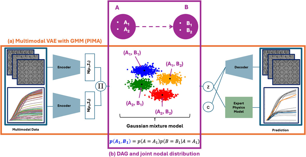
Figure 1. Cartoon description of the pimaDAG algorithm. Our algorithm uniquely links a Bayesian network (BN) prior (b) to the latent space clustering of a multimodal VAE (a). Each modality is variationally encoded into latent space by a unimodal encoder; unimodal embeddings are joined through a product of experts $(\mathrm{\Pi })$. Points in the latent space are clustered by a Gaussian mixture prior. Gaussian clusters are linked to a trainable BN by identifying each cluster with an outcome of the DAG nodes of the BN. More concretely, the probability of belonging to a given cluster is set equal to the probability of the associated DAG nodal outcome. For example, given a trainable DAG with nodes $A$ and $B$, the blue cluster is identified to the nodal outcome $(A_1,B_1)$, and thus, the probability of belonging to the blue cluster is equal to the probability $p(A=A_1,B=B_1)$. Points in the latent space are decoded back into each modality, with the option of incorporating known physics into the decoders.

For convenience, Table 1 in summarizes the notation used throughout this section and the rest of the paper.

Table 1

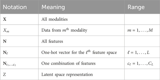
Table 1. List of notation for pimaDAG derivation.

2.1 Algorithmic framework

Given data $\mathbf{X}=\{X_1,\dots ,X_M\}$ from $M$ distinct modalities, we seek a common embedding into a latent space $Z\in {\mathbb{R}}^J$, where the latent space representation admits distinct clusters based on encoded features of the data. To model these clusters, we assume that $Z$ is a Gaussian mixture model (GMM). We identify our encoded GMM clusters with $L$ discrete features $\mathbf{N}=({\mathbf{N}}_1,\dots ,{\mathbf{N}}_L)$. The probability distribution of $\mathbf{N}$ forms the mixing probabilities of the GMM. In other words, if each feature ${\mathbf{N}}_{\ell }$ is a categorical random variable with $C_{\ell }$ outcomes and we let ${\mathbf{N}}_{c_1,\dots ,c_L}$ denote one outcome of $\mathbf{N}$, then $Z|\mathbf{N}={\mathbf{N}}_{c_1,\dots ,c_L}$ is normally distributed and has the probability of belonging. Moreover, we assume that there are shared latent dependencies between features and that these dependencies are described by a directed acyclic graph (DAG): each feature ${\mathbf{N}}_{\ell }$ is a node in a DAG $G$. Thus, by assuming the Markov factorization property,

$p\left(\mathbf{N}\right)≔p\left({\mathbf{N}}_1,\dots ,{\mathbf{N}}_L\right)={\displaystyle \prod _{\ell =1}^L}p\left({\mathbf{N}}_{\ell }|\text{Pa}\left({\mathbf{N}}_{\ell }\right)\right),(1)$

where $\text{Pa}({\mathbf{N}}_{\ell })$ denotes the immediate parents of feature node ${\mathbf{N}}_{\ell }$. Supplementary Figure S1 shows how the DAG of features relates to the latent space embedding.

For such a Gaussian mixture latent representation described by $Z$ and $\mathbf{N}$, we aim to construct our embedding and latent space representation through training a multimodal variational autoencoder. Following works such as Dilokthanakul et al. (2016), Jiang et al. (2017), and Walker et al. (2024), we train our VAE to find the prior distribution $p$, the posterior distribution $q$, the joint distribution of $\mathbf{N}$, and the DAG $G$, which maximize the evidence lower bound (ELBO) loss:

$\mathcal{L}={\mathbb{E}}_{q\left(Z,N|\mathbf{X}\right)}\left[\log \frac{p\left(\mathbf{X},Z,\mathbf{N}\right)}{q\left(Z,\mathbf{N}|\mathbf{X}\right)}\right].$

We assume independence of decoding mechanisms for each modality for our prior, and we assume mean-field separability for the posterior. These assumptions, respectively, give

$p\left(\mathbf{X}|Z,\mathbf{N}\right)={\displaystyle \prod _{m=1}^M}p\left(X_m|Z,\mathbf{N}\right)\text{\hspace{0.17em}and\hspace{0.17em}}q\left(Z,\mathbf{N}|\mathbf{X}\right)=q\left(Z|\mathbf{X}\right)q\left(\mathbf{N}|\mathbf{X}\right).(2)$

With these assumptions, the ELBO separates as sums of expectations of Gaussian distributions; see Equation 23. In the case of Gaussians with diagonal covariance, Jiang et al. (2017) gave a closed-form solution to compute such an expectation (see Corollary 5.1 in Supplementary Material 5). For general Gaussian distributions, we give the closed-form solution in Lemma 5.2 of Supplementary Material 5, but, for simplicity, we assume Gaussian distributions with diagonal covariances throughout this work.

Our algorithmic framework thus consists of (a) a multimodal VAE with a GMM prior and (b) a parameterization of our DAG and BN that ties into the GMM of (a), as highlighted in Figure 1. We describe each of these components in the subsections below.

2.1.1 Multimodal VAE with a GMM prior

Our multimodal representation learning framework amounts to a VAE with a GMM prior on the latent space; see the orange box (a) in Figure 1. Specifically, the latent space $Z$ is assumed to be a mixture of $C={\prod }_{\ell =1}^L{C}_{\ell }$ Gaussian distributions, where $L$ is the number of nodes and $C_{\ell }$ is the number of outcomes of the ${\ell }^{th}$ node ${\mathbf{N}}_{\ell }$. The joint probability on the mixture assignment in the GMM is additionally assumed to factorize with a Bayesian network prior to obey the Markov factorization property in Equation 1. Assignment to an individual cluster $(c_1,\dots ,c_L)$ has the probability

${\mathbf{A}}_{c_1,\dots ,c_L}≔p\left({\mathbf{N}}_{c_1,\dots ,c_L}\right)=p\left({\mathbf{N}}_1=c_1,{\mathbf{N}}_2=c_2,\dots ,{\mathbf{N}}_L=c_L\right),$

and each cluster in the GMM has a Gaussian distribution

$p\left(Z|{\mathbf{N}}_{c_1,\dots ,c_L}\right)\sim \mathcal{N}\left({\tilde{\mu }}_{c_1,\dots ,c_L},{\tilde{\sigma }}_{c_1,\dots ,c_L}^2\mathbf{I}\right),$

where the parameters ${\tilde{\mu }}_{c_1,\dots ,c_L}\in {\mathbb{R}}^J$ and ${\tilde{\sigma }}_{c_1,\dots ,c_L}^2\in {\mathbb{R}}^J$ are recovered by training with a first-order optimizer or computed using a block-coordinate maximization strategy outlined in Section 2.2.2.

The multimodal embedding and decoding of the VAE is similar to Walker et al. (2024). In particular, we use neural network encoders to embed each modality as a Gaussian and then combine these embeddings using a product of experts (see $\mathrm{\Pi }$ in Figure 1). In other words, for each modality $m$, we assume $q(Z|X_m)\sim \mathcal{N}({\mu }_m,{\sigma }_m^2\mathbf{I})$, where $[{\mu }_m,{\sigma }_m^2]=F_m(X_m;{\theta }_m)$ for a neural network $F_m$ with trainable parameters ${\theta }_m$. We deterministically compute the multimodal embedding from the unimodal ones via the identity

$q\left(Z|\mathbf{X}\right)\sim \mathcal{N}\left(\mu ,{\sigma }^2\mathbf{I}\right)=\alpha {\displaystyle \prod _{m=1}^M}\mathcal{N}\left({\mu }_m,{\sigma }_m^2\mathbf{I}\right),$

where $\alpha$ is a normalization constant, and

$\begin{array}{c}\hfill {\sigma }^{-2}={\displaystyle \sum _{m=1}^M}{\sigma }_m^{-2}\text{\hspace{0.17em}and\hspace{0.17em}}\frac{\mu }{{\sigma }^2}={\displaystyle \sum _{m=1}^M}\frac{{\mu }_m}{{\sigma }_m^2}.\end{array}$

During training, the multimodal distribution is sampled using the reparameterization trick. In other words, we sample $ϵ\sim \mathcal{N}(0,\mathbf{I})$ and compute $z=\mu +ϵ\odot \sigma$, where $\odot$ is the Hadamard product.

Our decoders output a Gaussian for each modality $p(X_m|Z,{\mathbf{N}}_{c_1,\dots ,c_L})\sim \mathcal{N}({\widehat{\mu }}_{m;c_1,\dots ,c_L},{\widehat{\sigma }}_{m;c_1,\dots ,c_L}^2\mathbf{I})$. The Gaussians’ parameters are determined by neural networks $D_{m;c_1,\dots ,c_L}$, i.e., $[{\widehat{\mu }}_{m;c_1,\dots ,c_L},{\widehat{\sigma }}_{m;c_1,\dots ,c_L}^2]=D_{m;c_1,\dots ,c_L}(Z;{\widehat{\theta }}_{m;c_1,\dots ,c_L})$. Alternatively our decoders $D_{m;c_1,\dots ,c_L}(Z;{\widehat{\theta }}_{m;c_1,\dots ,c_L})$ can be expert models, or they can depend upon only $Z$, i.e., $p(X_m|Z,{\mathbf{N}}_{c_1,\dots ,c_L})=p(X_m|Z)$.

2.1.2 Directed acyclic graph and joint distribution of nodes

The GMM prior in the previous section implicitly uses the Markov factorization property, which requires knowledge of a DAG to relate the causal dependencies between clusters; since we do not assume knowledge of this DAG a priori, we must recover this DAG and the accompanying probability distribution of the resulting BN while simultaneously training our VAE. We first describe our DAG parameterization, followed by our method to compute the resulting joint probability distribution.

Our DAG parameterization builds off of concepts from Hodge theory (Jiang et al., 2011; Lim, 2020). We parameterize an edge indicator function as the graph gradient $(\mathcal{G})$ on a set of nodes. By using the graph gradient, we guarantee that our edge indicator function is curl-free, and consequently, we define a complete DAG; we introduce sparsity in the complete DAG through nonnegative weightings $(B)$ of edges.

As a brief summary, Hodge theory provides a generalization for vector calculus concepts of gradient, curl, and divergence, and discrete Hodge theory generalizes these notions to the discrete setting of graphs to define the graph gradient, graph curl, graph divergence, etc. Through these definitions, we can view numeric labels on nodes and edges as functions on the nodes and edges, respectively. If we define the functions on the edges to be the graph gradient of the edge’s adjacent node values, then we view the edges as the flow between the nodal values. Furthermore, by defining edge values via the graph gradient, we ensure that our edges define a curl-free function, which means that our edge values define a DAG since curl-free functions on graphs have no cycles by construction. We note that the graph gradient will define a complete DAG, so we use trainable nonnegative coefficients $(B)$ to introduce sparsity. For more information on Hodge theory and the generalization to graphs, see Trask et al. (2020); Lim (2020).

Explicitly, given a set of nodes, our DAG parameterization assigns a trainable scalar score ${\xi }_{\ell }$ to each node ${\mathbf{N}}_{\ell }$. We denote the vector of trainable node scores as $\vec{\xi }$. Each potential edge $E_{ij}$ between nodes is assigned a value $F_{ij}$ given by

$\begin{array}{c}\hfill F_{ij}={\left(B\cdot \mathcal{G}\xi \right)}_{ij}=B_{ij}\left({\xi }_j-{\xi }_i\right),\end{array}$

where $\mathcal{G}$ is the graph gradient operator, and each $B_{ij}$ is a trainable nonnegative scalar used to induce sparsity in $G$. In terms of Hodge theory, one can view $B$ as an $L\times L$ trainable nonnegative metric tensor and $F_{ij}$ as a flow from node ${\mathbf{N}}_j$ to node ${\mathbf{N}}_i$.

We use these edge values $F_{ij}$ to give a regularized edge indicator function:

$E_{ij}=\text{ReLU}\left(\tanh \left(\frac{1}{\beta }{F}_{ij}\right)\right),(3)$

where the scalar $\beta >0$ is a temperature parameter that controls the sharpness of the regularization of the indicator function. We use this temperature to control how easily the DAG can update during training, as described in Section 2.2.3. With this formulation, we assign edges in our DAG via the rule

${\mathbf{N}}_i\subseteq \text{Pa}\left({\mathbf{N}}_j\right)\Leftarrow \Rightarrow {\lim }_{\beta \to 0}{E}_{ij}=1\Leftarrow \Rightarrow B_{ij}\ne 0\text{\hspace{0.17em}and\hspace{0.17em}}{\xi }_i<{\xi }_j.(4)$

Theorem 2.1. Let A be the adjacency matrix of a directed graph G. Then G is a DAG if and only if $\mathbf{A}={\lim }_{\beta \to 0}E$ for some matrix E with entries given by Equation 3.

Our DAG parameterization does guarantee a DAG, and parameterization is flexible enough to learn any possible DAG. Formal proofs are given in Supplementary Material 3.

Proof: see Lemma 3.4 and Proposition 3.6 in Supplementary Material 3.

We now proceed to compute the joint probability distribution on $\mathbf{N}$ as per the Markov factorization property. This means that we must parametrize the probability distribution at each node ${\vec{\pi }}_{\ell }=p({\mathbf{N}}_{\ell }|\text{Pa}({\mathbf{N}}_{\ell }))$ and have a method for computing $p(\mathbf{N})$ from ${\vec{\pi }}_{\ell }$. Our parametrization must be flexible enough to allow for the direction of the edge dependencies in the DAG $G$ to change during training, and, as a result, the number of causal factors that are parents of a given node (i.e., $\text{Pa}({\mathbf{N}}_{\ell })$) may change as well. We therefore build, for each node ${\mathbf{N}}_{\ell }$, a parameterization of these probabilities that allows for any subset of nodes to be parents via a trainable tensor ${\mathbf{W}}^{\ell }$; we downselect which nodes are parents by using the DAG edge indicator scores from Equation 3 and averaging out those modes that are not parents. For ease of notation, we let $\mathbf{A}=p(\mathbf{N})$.

For each $\ell =1,\dots ,L$, we define ${\mathbf{W}}^{\ell }$ to be a nonnegative rank-$L$ tensor of size $C_1\times \cdots \times C_L$ constrained so that for any $c_1,\dots ,c_{\ell -1},c_{\ell +1},\dots ,c_L$,

${\displaystyle \sum _{c_{\ell }=1}^{C_{\ell }}}{W}_{c_1,\dots ,c_L}^{\ell }=1.$

This constraint ensures that the entries of ${\mathbf{W}}^{\ell }$ represent the probabilities

$\begin{array}{cc}\hfill {\mathbf{W}}^{\ell }:& =p\left({\mathbf{N}}_{\ell }|{\mathbf{N}}_k\text{\hspace{0.17em}for\hspace{0.17em}}k\ne \ell \right)\hfill \\ \hfill W_{c_1,\dots ,c_L}^{\ell }& =p\left({\mathbf{N}}_{\ell }={\mathbf{1}}_{c_{\ell }}|{\mathbf{N}}_k={\mathbf{1}}_{c_k}\text{\hspace{0.17em}for\hspace{0.17em}}k\ne \ell \right),\hfill \end{array}$

where ${\mathbf{1}}_c$ is a one-hot encoding, with the $c^{\text{th}}$ entry set to 1.

With this definition, we now proceed to describe our downselection algorithm for parameterizing the probabilities over the structure of a given DAG. If a node ${\mathbf{N}}_k$ is not a parent node of ${\mathbf{N}}_{\ell }$, then we remove mode $k$ from ${\mathbf{W}}^{\ell }$ by contracting ${\mathbf{W}}^{\ell }$ against $\frac{1}{C_k}\mathbf{1}$ (where $\mathbf{1}$ is the vector of all ones) along mode $k$. In essence, we are replacing the mode $k$ in ${\mathbf{W}}^{\ell }$ by its average. This contraction makes ${\mathbf{N}}_{\ell }$ independent of ${\mathbf{N}}_k$ when ${\mathbf{N}}_k$ is not a parent of ${\mathbf{N}}_{\ell }$. If the node ${\mathbf{N}}_k$ is a parent of ${\mathbf{N}}_{\ell }$, then we can contract against the realizations of the parent one-hot encodings since they are already known. We, therefore, end up with an expression for the categorical distribution on ${\mathbf{N}}_{\ell }|\text{Pa}({\mathbf{N}}_{\ell })$ via

$\begin{array}{cc}\hfill {\vec{\pi }}_{\ell }=p\left({\mathbf{N}}_{\ell }|\text{Pa}\left({\mathbf{N}}_{\ell }\right)\right)& ={\mathbf{W}}^{\ell }{\bar{\times }}_1{v}_1{\bar{\times }}_2{v}_2\dots {\bar{\times }}_{\ell -1}{v}_{\ell -1}{\bar{\times }}_{\ell +1}{v}_{\ell +1}\dots {\bar{\times }}_L{v}_L\hfill \\ \hfill & ={\displaystyle \sum _{\begin{array}{c}k=1\\ k\ne \ell \end{array}}^L}{\displaystyle \sum _{c_k=1}^{C_k}}{W}_{c_1,\dots ,c_L}^{\ell }{v}_{k,c_k},\hfill \end{array}$

where ${\bar{\times }}_k$ denotes the contractive $n$-mode tensor product against mode $k$ (see Kolda and Bader (2009); Bader and Kolda (2006) for more details), and

$v_k=\left\{\begin{array}{cc}{\mathbf{N}}_k\hfill & \text{\hspace{0.17em}if\hspace{0.17em}}{\mathbf{N}}_k\subseteq \text{Pa}\left({\mathbf{N}}_{\ell }\right)\hfill \\ \frac{1}{C_k}\mathbf{1}\hfill & \text{\hspace{0.17em}if\hspace{0.17em}}{\mathbf{N}}_k\subseteq \text{Pa}{\left({\mathbf{N}}_{\ell }\right)}^{\mathbf{c}}\text{\hspace{0.17em}and\hspace{0.17em}}k\ne \ell .\hfill \end{array}\right.$

Using our DAG representation, these cases can be written as follows:

$v_k=\left\{\begin{array}{cc}{\mathbf{N}}_k\hfill & \text{\hspace{0.17em}if\hspace{0.17em}}{E}_{k,\ell }=1\hfill \\ \frac{1}{C_k}\mathbf{1}\hfill & \text{\hspace{0.17em}if\hspace{0.17em}}{E}_{k,\ell }\ne 1\text{\hspace{0.17em}and\hspace{0.17em}}k\ne \ell ,\hfill \end{array}\right.$

or more concisely as

$v_k=\frac{1}{C_k}\mathbf{1}-E_{k,\ell }\left(\frac{1}{C_k}\mathbf{1}-{\mathbf{N}}_k\right)\text{\hspace{0.17em}for\hspace{0.17em}}k\ne \ell ,$

which has the benefit of allowing us to handle relaxations of $E$ when $E$ is not necessarily a binary matrix (such as when the temperature $\beta$ is small but not yet sufficiently close to 0). With $v_k$ defined as such, we can write ${\vec{\pi }}_{\ell }$ via

${\vec{\pi }}_{\ell }={\displaystyle \sum _{\begin{array}{c}k=1\\ k\ne \ell \end{array}}^L}{\displaystyle \sum _{c_k=1}^{C_k}}{W}_{c_1,\dots ,c_L}^{\ell }{\left(\frac{1}{C_k}\mathbf{1}-E_{k,\ell }\left(\frac{1}{C_k}\mathbf{1}-{\mathbf{N}}_k\right)\right)}_{c_k}.(5)$

From the tensors ${\mathbf{W}}^{\ell }$ and the vectors ${\vec{\pi }}_{\ell }$, we can now compute $\mathbf{A}$.

By Corollary 3.5, we may assume that the categorical variables ${\mathbf{N}}_1,\dots ,{\mathbf{N}}_L$ are ordered such that $\forall k<\ell$, ${\mathbf{N}}_k\subset \text{Anc}({\mathbf{N}}_{\ell })$; if not, we reassign the indices via the permutation $\sigma$. Observe that, by assumption of the Markov factorization property,

$\begin{array}{cc}\hfill {\mathbf{A}}^{\ell }& ≔p\left({\mathbf{N}}_1,\dots ,{\mathbf{N}}_{\ell }\right)\hfill \\ \hfill & =p\left({\mathbf{N}}_{\ell }|\text{Pa}\left({\mathbf{N}}_{\ell }\right)\right){\mathbf{A}}^{\ell -1},\hfill \end{array}$

where ${\mathbf{A}}^0=1$ and where the expression for $p({\mathbf{N}}_{\ell }|\text{Pa}({\mathbf{N}}_{\ell }))$ is given by ${\vec{\pi }}_{\ell }$ in Equation 5. This inductive process of computing $\mathbf{A}={\mathbf{A}}^L$ is given in Algorithm 1.

Algorithm 1.Algorithm for computing joint distribution kernel $\mathbf{A}$.

 Require: $E$ an upper-triangular DAG score matrix

 Require: ${\mathbf{W}}^1,\dots ,{\mathbf{W}}^L$ tensors, where ${\mathbf{W}}^{\ell }=p({\mathbf{N}}_{\ell }|{\mathbf{N}}_k\text{\hspace{0.17em}for\hspace{0.17em}}k\ne \ell )$

  ${\mathbf{A}}^0$ = 1

  for $\ell =1$ to $L$ do

   ${\mathbf{W}}^{\ell }\leftarrow \mathtt{r}\mathtt{e}\mathtt{d}\mathtt{u}\mathtt{c}\mathtt{e}\text{\_}\mathtt{m}\mathtt{e}\mathtt{a}\mathtt{n}({\mathbf{W}}^{\ell },\mathtt{a}\mathtt{x}\mathtt{i}\mathtt{s}=[\ell +1,\dots ,L],\mathtt{k}\mathtt{e}\mathtt{e}\mathtt{p}\mathtt{d}\mathtt{i}\mathtt{m}\mathtt{s}=\mathtt{F}\mathtt{a}\mathtt{l}\mathtt{s}\mathtt{e})$

   for $k=1$ to $\ell -1$ do

    ${\mathbf{W}}^{\ell }\leftarrow E_{\ell ,k}\cdot {\mathbf{W}}^{\ell }+(1.0-E_{\ell ,k})\cdot \mathtt{r}\mathtt{e}\mathtt{d}\mathtt{u}\mathtt{c}\mathtt{e}\text{\_}\mathtt{m}\mathtt{e}\mathtt{a}\mathtt{n}({\mathbf{W}}^{\ell },\mathtt{a}\mathtt{x}\mathtt{i}\mathtt{s}=\mathtt{k},\mathtt{k}\mathtt{e}\mathtt{e}\mathtt{p}\mathtt{d}\mathtt{i}\mathtt{m}\mathtt{s}=\mathtt{T}\mathtt{r}\mathtt{u}\mathtt{e})$

   end for

   ${\mathbf{A}}^{\ell }\leftarrow {\mathbf{W}}_{\dots ,:}^{\ell }\odot {\mathbf{A}}^{\ell -1}$

  end for

 output $\mathbf{A}\leftarrow {\mathbf{A}}^L$

As a result of Algorithm 1, we have flexible parameterization for the joint distribution on $\mathbf{N}$, which is used for the GMM mixing probabilities in our VAE. This parameterization, of both $\mathbf{N}$ and the underlying DAG, are differentiable and amenable to automatic differentiation, allowing us to train in an end-to-end fashion. Our training approach is described in the next section.

2.2 ELBO loss and training

We now describe the loss function used to train pimaDAG. The ELBO loss for training is similar to that of Walker et al. (2024), albeit with a different notation and an additional computation of cluster assignment based on the DAG.

2.2.1 Single-sample ELBO

The full ELBO derivation is in Supplementary Material 4. After dropping constant terms, the single-sample ELBO is

$\begin{array}{cc}\hfill \mathcal{L}& =-{\displaystyle \sum _{m=1}^M}\log \left({\widehat{\sigma }}_m^2\right)+{‖\frac{X_m-{\widehat{\mu }}_m}{{\widehat{\sigma }}_m}‖}^2+{\displaystyle \sum _{j=1}^J}\log \left({\sigma }_j^2\right)\hfill \\ \hfill & +{\displaystyle \sum _{c_1=1}^{C_1}}\cdots {\displaystyle \sum _{c_L=1}^{C_L}}{\gamma }_{c_1,\dots ,c_L}\cdot \left[2\log \left(\frac{{\mathbf{A}}_{c_1,\dots ,c_L}}{{\gamma }_{c_1,\dots ,c_L}}\right)-{\displaystyle \sum _{j=1}^J}\log \left({\tilde{\sigma }}_{c_1,\dots ,c_L;j}^2\right)\right.\hfill \\ \hfill & +\frac{{\sigma }_j^2}{{\tilde{\sigma }}_{c_1,\dots ,c_L;j}^2}+\left(+\frac{{\left({\mu }_j-{\tilde{\mu }}_{c_1,\dots ,c_L;j}\right)}^2}{{\tilde{\sigma }}_{c_1,\dots ,c_L;j}^2}\right),\hfill \end{array}(6)$

where ${\gamma }_{c_1,\dots ,c_L}$ is an estimate for the posterior distribution $q(\mathbf{N}|\mathbf{X})$ and, following Jiang et al. (2017), is computed by

$\begin{array}{cc}\hfill \gamma :& =q\left(\mathbf{N}|\mathbf{X}\right)=p\left(\mathbf{N}|Z\right)=\frac{p\left(\mathbf{N}\right)p\left(Z|\mathbf{N}\right)}{p\left(Z\right)}\hfill \\ \hfill {\gamma }_{c_1,\dots ,c_L}& =\frac{p\left({\mathbf{N}}_{c_1,\dots ,c_L}\right)p\left(Z|{\mathbf{N}}_{c_1,\dots ,c_L}\right)}{{\sum }_{c_1^{\prime }=1}^{C_1}\cdots {\sum }_{c_L^{\prime }=1}^{C_L}p\left({\mathbf{N}}_{c_1^{\prime },\dots ,c_L^{\prime }}\right)p\left(Z|{\mathbf{N}}_{c_1^{\prime },\dots ,c_L^{\prime }}\right)}\hfill \\ \hfill & =\frac{{\mathbf{A}}_{c_1,\dots ,c_L}p\left(Z|{\mathbf{N}}_{c_1,\dots ,c_L}\right)}{{\sum }_{c_1^{\prime }=1}^{C_1}\cdots {\sum }_{c_L^{\prime }=1}^{C_L}{\mathbf{A}}_{c_1^{\prime },\dots ,c_L^{\prime }}p\left(Z|{\mathbf{N}}_{c_1^{\prime }\dots c_L^{\prime }}\right)},\hfill \end{array}(7)$

where we recall $\mathbf{A}≔p(\mathbf{N})$ for convenience. Note that $\mathbf{A}$ and $\gamma$ are both tensors with $L$ modes of size $C_1\times \cdots \times C_L$. The tensor $\mathbf{A}$ can be calculated via Algorithm 1 in Section 2.1.2. The values of $p(Z|\mathbf{N})$ can be computed by sampling from each Gaussian in the Gaussian mixture model. All other values are parameters in our model. Table 2 summarizes the assumed distributions on each term in the architecture and lists how the variables are computed and updated during training.

Table 2

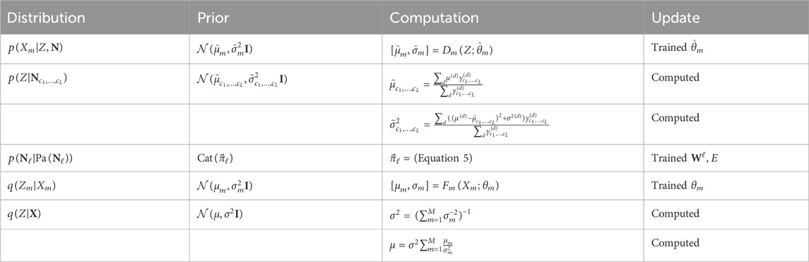
Table 2. Choices of distributions.

2.2.2 Training

To train our causal model, we seek to maximize the ELBO $\mathcal{L}$ over the entire dataset. In other words, if we use ${\mathcal{L}}_d$ to denote Equation 6 for the $d^{th}$ datapoint, then we want to minimize $-{\sum }_d{\mathcal{L}}_d$. Throughout training, we alternate between (1) updating the neural network, expert model, and DAG parameters via gradient descent and (2) updating the Gaussian mixture centers and variances using block-coordinate maximization, similar to Walker et al. (2024). In particular, we compute the optimal Gaussian mixture centers and variances by taking the derivative of $-{\sum }_d{\mathcal{L}}_d$ with respect to these parameters and solving for the global minimizers:

$\begin{array}{cc}\hfill {\tilde{\mu }}_{c_1,\dots ,c_L}& =\frac{{\sum }_d{\mu }^{\left(d\right)}{\gamma }_{c_1,\dots ,c_L}^{\left(d\right)}}{{\sum }_d{\gamma }_{c_1,\dots ,c_L}^{\left(d\right)}},\hfill \\ \hfill {\tilde{\sigma }}_{c_1,\dots ,c_L}^2& =\frac{{\sum }_d\left({\left({\mu }^{\left(d\right)}-{\tilde{\mu }}_{c_1,\dots ,c_L}\right)}^2+{\sigma }^{2\left(d\right)}\right){\gamma }_{c_1,\dots ,c_L}^{\left(d\right)}}{{\sum }_d{\gamma }_{c_1,\dots ,c_L}^{\left(d\right)}},\hfill \end{array}(8)$

where $d$ indexes the $d^{th}$ data point, and, in particular, ${\mu }^{(d)}$ and ${\sigma }^{2(d)}$ are, respectively, the encoded mean and variance of the $d^{th}$ data point. Our training procedure follows Algorithm 2.

Algorithm 2.Training algorithm for pimaDAG.

 input data $\mathrm{x}=\{X_1,\dots ,X_M\}$ in batches $\mathcal{B}$

  Compute ${\gamma }_{c_1,\dots ,c_L}^{(d)}$ for all $x^{(d)}\in \mathrm{x}$ via Equation 7

  Compute ${\tilde{\mu }}_{c_1,\dots ,c_L}$ and ${\tilde{\sigma }}_{c_1,\dots ,c_L}^2$ via Equation 8

  for $i=1$ to $N_{\mathit{epochs}}$ do

   for $b\in \mathcal{B}$ do

    Perform optimizer update on ELBO

   end for

   Calculate ${\gamma }_{c_1,\dots ,c_L}$ for all $x^{(d)}\in \mathrm{x}$ via Equation 7

   Update ${\tilde{\mu }}_{c_1,\dots ,c_L}$ and ${\tilde{\sigma }}_{c_1,\dots ,c_L}^2$ via Equation 8

  end for

2.2.3 Practical considerations

We implement several tools for aiding training and algorithm adaptation. These tools are described here, and the use of these tools in each experiment is detailed in Supplementary Material 2.

2.2.3.1 Pre-training

We sometimes found that before fitting a DAG, we need a reasonable latent embedding, in the sense that the DAG is meant to relate informative latent features instead of random features at initialization. Thus, we implemented an optional pre-training regimen, following Jiang et al. (2017) and Kingma and Welling (2014). As our first step in pre-training, we fix the pre-initialized encoders and initialize the cluster means and variances via Equations 7, 8. This initialization has the benefits of providing a good GMM fit for the initial latent embedding, but if the initial latent embedding is poor or undiscriminating, then the initial GMM fitting by these steps might not focus on any informative features. Our next step in pre-training is to train the weights and biases of the encoders and decoders via the reconstruction term or by fitting a unit-normal Gaussian variational autoencoder (Kingma and Welling, 2014). Following this training, we find a good initial GMM fit through iterations of Equations 7, 8. This has the benefit of finding a good initial embedding, from which block-coordinate maximization can recover meaningful features.

2.2.3.2 Edge indicator function adaptations

We have two optional adaptations to the edge indicator function. The first is to add random noise to the node scores $\mathit{\xi }$. This noise is included to break free of local minima and may additionally test edge orientation. Our second adaptation is to anneal $\beta$ during training. In Equation 3, $\beta$ serves as a temperature parameter, and, as $\beta \to 0$, $E$ approaches a true indicator function. Our annealing implementation is simple, where we specify the initial $\beta$, the final $\beta$, and the update frequency of $\beta$.

2.2.3.3 Updates on GMM parameters

The cluster center and variance updates in Equation 8, paired with the gamma calculation in Equation 7, are reminiscent of expectation-maximization. The traditional maximization step would, however, also update the probability of belonging to each cluster $(\mathbf{A})$. Although there is no closed-form expression for an update on $\mathbf{A}$ from our ELBO since they depend on the underlying causal factorization, we alternatively perform extra gradient-descent steps to update $\mathbf{A}$ after each update of the cluster means and variances. Furthermore, we also implemented the option to perform multiple iterations of GMM variable updates per epoch.

3 Results

Although we prove in Proposition 3.6 that our DAG parameterization is capable of learning any DAG, we demonstrate this capability in Section 3.1. We then test pimaDAG on a synthetic dataset consisting of circle images and a scientific dataset consisting of 3D-printed lattices. All architectures, hyperparameters, and training details for the experiments can be found in Supplementary Material 2.

3.1 Efficacy of DAG parameterization

We test the ability of our DAG parameterization (Equation 3) to recover any DAG. First, we generate a random set of DAGs of various sizes, i.e., the number of nodes $L=\{\mathrm{6,12,24,48}\}$, by generating a (random) consistent ordering, inducing a DAG on the complete graph of $L$ nodes, and then randomly discarding edges from the complete graph by a Bernoulli distribution with probability $p=0.25$ that an edge is discarded. For each graph in our dataset, we train to recover the specified DAG’s adjacency matrix, comparing the edge adjacency matrix of the predicted graph to that of the true graph using binary cross-entropy (BCE) as our loss and Adam as our optimizer. We use a learning rate of $\lambda =0.001$ and train for $25K$ steps with a batch size of 16. For the largest size $L=48$, training was extended to $50K$ steps as the loss had not converged after the first $25K$ steps; this slowdown in convergence is expected, given that the number of unique DAGs grows superexponentially with the number of vertices in a graph (Kuipers and Moffa, 2015). Training begins with an initial temperature $\beta$ of 0.5, and we reduce $\beta$ by 1% every 100 steps to a minimum temperature of ${\beta }_{\text{min}}=0.001$. We repeat this test for $N_{\text{samples}}=20$ for each size graph. In Table 3, we report the average and standard deviation of the BCE loss for each of the sampled DAGs for each size. In every sample at every size in our test, with the exception of a single sample for $L=48$, the largest graph size, we recover the adjacency matrix within $1.0\times 10^{-4}$ entry-wise accuracy, often with accuracies of $10^{-6}$ or smaller; the maximum absolute entry-wise error (MAE) in the predicted adjacency graph across all entries and all samples of that size is also reported in Table 3. Similar statistics are shown for common test DAGs, taken from the BNLearn (Scutari, 2010) repository of Bayesian networks, yielding comparable results, as shown in Table 4.

Table 3

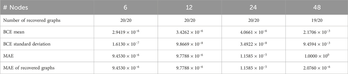
Table 3. Training performance on DAG recovery tests from randomly generating graphs in experiment 3.1 for DAGs of various sizes.

Table 4

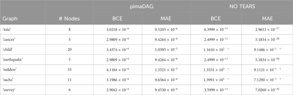
Table 4. Training performance on DAG recovery tests for various DAGs from the BNLearn repository in experiment 3.1 comparing our pimaDAG algorithm against NO TEARS. Results marked with a dagger $†$ denote that the algorithm failed to return a DAG.

We additionally compare our ability to recover the DAG adjacency matrix against NO TEARS (Zheng et al., 2018) on the same benchmarks in Table 4 using the same metrics for success used in Table 3. To make pimaDAG and NO TEARS comparable, we do not perform any optional enhancement of the discovered DAG in Zheng et al. (2018), such as weight thresholding or $L^1$ regularization, and we otherwise use the same parameterization, as provided for in their original work. We note a handful of key differences between these two methods, namely, that (1) pimaDAG’s parameterization yields an unconstrained nonlinear optimization problem, while NO TEARS yields a linear problem (depending on choice of loss, as described in Zheng et al. (2018)) with a nonlinear constraint; (2) pimaDAG uses a first-order optimizer, while NO TEARS uses a second-order optimizer as part of an augmented Lagrangian scheme; and (3) pimaDAG always guarantees a DAG by construction, while NO TEARS guarantees a DAG only when the constraints are satisfied, which is not guaranteed a priori in the augmented Lagrangian formulation. Thus, we see in Table 4 that when NO TEARS successfully finds a DAG, it generally does so more efficiently and accurately, which is unsurprising given its more sophisticated optimization approach but that for the larger graphs $(N>10)$ tested from the BNLearn repository, NO TEARS fails to recover a DAG and generally performs poorly on these problems. This behavior motivates the need for methods like pimaDAG, which guarantee a DAG by construction during all stages of end-to-end training.

3.2 Circles

For our first pimaDAG experiment, we generated a synthetic unimodal dataset consisting of images of circles with three different features: hue $h$ (red and blue), radius $r$ (Gaussian mixture of big and small), and shift $s$ (Gaussian mixture of left and right). We generated 4,096 circles using the decision tree in Supplementary Figure S2 where we purposefully overlapped distributions of $h$, $r$, and $s$ to necessitate the discovery of a DAG describing the generative process. We ran this experiment with three nodes in the DAG, where each node was a binary categorical random variable. The latent space showed disentanglement in the three different features. The learned DAG is in subpanel (E) of Figure 2. By comparing cluster labels to features characteristic of each cluster, we see that node ${\mathbf{N}}_1$ in the DAG corresponds to the radius, node ${\mathbf{N}}_2$ corresponds to the hue, and node ${\mathbf{N}}_3$ corresponds to the shift. For example, we conclude that ${\mathbf{N}}_2$ corresponds to the hue as all clusters with red circles have a 0 in the second entry of their label. Under this identification, the resulting directed acyclic graph demonstrates that the radius and hue play a key role in the outcome of the shift.

Figure 2

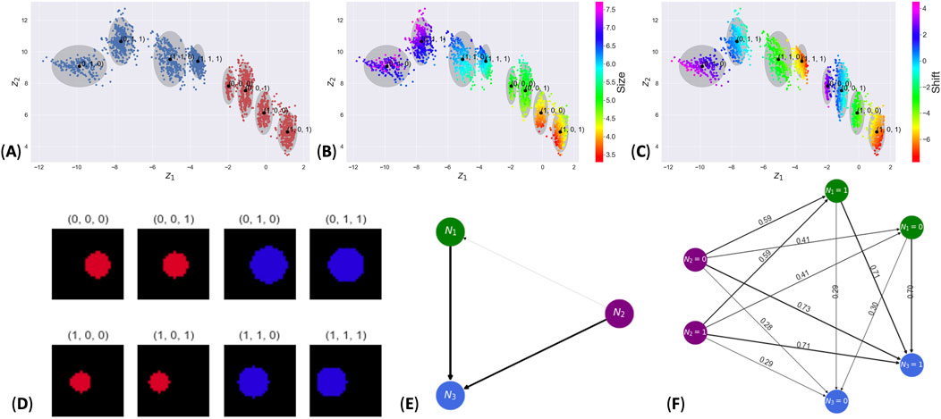
Figure 2. Results from the synthetic circles dataset. Subpanels (A–C) show the latent space colored by hue, radius, and shift, respectively. Panel (D) shows the image of the datapoint nearest the cluster mean for each cluster. Subpanel (E) contains the learned DAG where edges are weighted by the probability of each edge. Subpanel (F) gives the probability of feature node ${\mathbf{N}}_{\ell }=n$, given the parent node ${\mathbf{N}}_j=m$. By identifying key features in each cluster with its label, we see that ${\mathbf{N}}_1$ represents the circle radius, ${\mathbf{N}}_2$ represents the hue, and ${\mathbf{N}}_3$ represents the shift.

3.3 Lattices

Our next experiment uses a dataset of 3D-printed lattices (Garland et al., 2020). In this dataset, two different lattice geometries were printed (octet and gyroid) from 316 L stainless steel, where each respective geometry was printed using the same 3D model but different print process parameters. Each lattice was a 10-mm cube with three $3\times 3$ unit cells. Strut diameters for the octets and wall thicknesses for the gyroids were both 0.5 mm in the model design. Although wall thicknesses and strut diameters were set to 0.5 mm, actual thicknesses and diameters varied due to the varied print process parameters. This dataset included a total of 91 printed lattices, where two modalities for each lattice sample were collected: an image $(X_1)$ of the lattice and a stress–strain curve produced by a high-throughput uniaxial compression machine $(X_2)$. The stress–strain curves represent a physics-imbued modality, where curves can be modeled via continuous piecewise linear functions; see Trask et al. (2022). Consequently, for the stress–strain modality, we used an expert model decoder composed of two piecewise linear segments. Specifying two binary feature nodes resulted in a latent space organized by the lattice type and stress–strain curves, see Figure 3. The two clusters consisting of the octet geometry merged, and the corresponding expert models are nearly identical. This result is consistent with the distribution of octet stress–strain curves, which has a lower variance than the gyroid stress–strain curves. By comparing cluster labels to features characteristic of each cluster, we see that node ${\mathbf{N}}_2$ corresponds to the lattice type while ${\mathbf{N}}_1$ corresponds to the stress–strain curve profile. The learned DAG suggests that the lattice type influences the stress–strain curve.

Figure 3

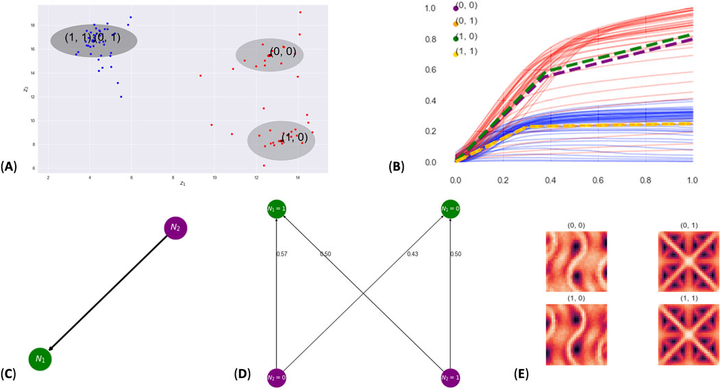
Figure 3. Results from the lattice experiment. Subpanel (A) shows the latent space, where two standard deviations for each cluster are shown as gray ellipses. Points in the latent space are colored by lattice type: gyroid (red) and octet (blue). Subpanel (B) shows the stress–strain curves colored by lattice type (gyroid in red and octet in blue) and the expert model for each cluster shown by dashed lines. Subpanel (C) shows the learned DAG; subpanel (D) shows the probability of feature node ${\mathbf{N}}_{\ell }=n$, given the parent node ${\mathbf{N}}_j=m$. Subpanel (E) shows the mean of each cluster decoded as an image. By comparing the cluster labels with the nodes of the graph, we see that ${\mathbf{N}}_2$ corresponds to the lattice type and influences ${\mathbf{N}}_1$, which corresponds to the stress–strain curve. This suggests that the mechanical response (stress–strain curve) follows from the microstructure imagery.

By way of comparison, note that Trask et al. (2022) tested PIMA on this same lattice dataset. In their Figure 6, they found two clusters: one for each lattice type. Their latent space provided a disentanglement of the data but did not give the additional insight given by our DAG, which identifies dependencies between stress–strain profiles and the lattice type. We thus anticipate that pimaDAG can aid in the discovery of hidden, dependent features in scientific datasets.

4 Conclusion

We present a general-purpose framework, pimaDAG, for discovering a Bayesian network of latent features in high-dimensional data. This framework is capable of handling multiple modalities and physics constraints to encourage disentanglement of data with a conditional independence structure. We introduce a new parameterization for learning DAGs, and we prove that this parameterization is capable of discovering any DAG; for a selection of DAGs, we confirm this via numerical experiments. We demonstrate the efficacy of pimaDAG on synthetic and real data, and we were able to achieve interpretable dependent features. These results show that meaningful disentanglement via a trainable Bayesian network is possible, even in purely exploratory settings.

There are some limitations to this framework. First, our model assumes discrete features, which means it may be less suitable for continuous features. Next, variational autoencoders are notoriously difficult to train to identify features amenable to analysis or that match extant intuition. In part, this follows from the fact that variational autoencoders only provide interpretable latent representations under certain constraints. Although the aim of this work was to discover a Bayesian network and its feature nodes for general data, with perhaps multiple modalities and physics constraints to provide pseudo-labels, future work will investigate the conditions necessary to generate unique features and conditional relationships within pimaDAG. We furthermore plan to investigate the possibility of including interventional data.

Data availability statement

The raw data supporting the conclusions of this article will be made available by the authors, without undue reservation.

Author contributions

EW: conceptualization, formal analysis, investigation, methodology, software, visualization, writing–original draft, and writing–review and editing. JA: conceptualization, formal analysis, investigation, methodology, software, visualization, writing–original draft, and writing–review and editing. CM: data curation, software, visualization, writing–original draft, and writing–review and editing. NT: conceptualization, funding acquisition, project administration, supervision, writing–original draft, and writing–review and editing.

Funding

The author(s) declare that financial support was received for the research, authorship, and/or publication of this article. All authors acknowledge funding under the Beyond Fingerprinting Sandia Grand Challenge Laboratory Directed Research and Development program as well as funding under the U.S. Department of Energy ASCR SEACROGS MMICCS Center.

Acknowledgments

The authors thank Brad Boyce, Remi Dingreville, Anthony Garland, Laura Swiler, Anthony Gruber, and Eric Cyr for support and helpful conversations and Kat Reiner for computing support. This article has been co-authored by employees of National Technology & Engineering Solutions of Sandia, LLC, under Contract No. DE-NA0003525, with the U.S. Department of Energy (DOE). The employees co-own all right, title, and interest in and to the article and are solely responsible for its contents. The United States Government retains and the publisher, by accepting the article for publication, acknowledges that the United States Government retains a non-exclusive, paid-up, irrevocable, world-wide license to publish or reproduce the published form of this article or allow others to do so, for United States Government purposes. The DOE will provide public access to these results of federally sponsored research in accordance with the DOE Public Access Plan https://www.energy.gov/downloads/doe-public-access-plan. Any subjective views or opinions that might be expressed in the paper do not necessarily represent the views of the U.S. Department of Energy or the United States Government. SAND NUMBER: SAND2023-11515O.

Conflict of interest

The authors declare that the research was conducted in the absence of any commercial or financial relationships that could be construed as a potential conflict of interest.

Publisher’s note

All claims expressed in this article are solely those of the authors and do not necessarily represent those of their affiliated organizations, or those of the publisher, the editors, and the reviewers. Any product that may be evaluated in this article, or claim that may be made by its manufacturer, is not guaranteed or endorsed by the publisher.

Supplementary material

The Supplementary Material for this article can be found online at: https://www.frontiersin.org/articles/10.3389/fmech.2024.1408649/full#supplementary-material

References

Bader, B. W., and Kolda, T. G. (2006). Algorithm 862: matlab tensor classes for fast algorithm prototyping. ACM Trans. Math. Softw. (TOMS) 32, 635–653. doi:10.1145/1186785.1186794

CrossRef Full Text | Google Scholar

Bengio, Y., Courville, A., and Vincent, P. (2013). Representation learning: a review and new perspectives. IEEE Trans. Pattern Analysis Mach. Intell. 35, 1798–1828. doi:10.1109/TPAMI.2013.50

PubMed Abstract | CrossRef Full Text | Google Scholar

Boyce, B. L., and Uchic, M. D. (2019). Progress toward autonomous experimental systems for alloy development. MRS Bull. 44, 273–280. doi:10.1557/mrs.2019.75

CrossRef Full Text | Google Scholar

Buchholz, S., Rajendran, G., Rosenfeld, E., Aragam, B., Sch olkopf, B., and Ravikumar, P. (2023). Learning linear causal representations from interventions under general nonlinear mixing. NeurIPS.

Google Scholar

Chickering, D. M., Heckerman, D., and Meek, C. (2004). Large-sample learning of bayesian networks is np-hard. J. Mach. Learn. Res.

Google Scholar

Dilokthanakul, N., Mediano, P. A., Garnelo, M., Lee, M. C., Salimbeni, H., Arulkumaran, K., et al. (2016). Deep unsupervised clustering with Gaussian mixture variational autoencoders. arXiv Prepr. arXiv:1611.02648. doi:10.48550/arXiv.1611.02648

CrossRef Full Text | Google Scholar

Gao, T., Bhattacharjya, D., Nelson, E., Liu, M., and Yu, Y. (2022). Idyno: learning nonparametric dags from interventional dynamic data. Int. Conf. Mach. Learn.

Google Scholar

Garland, A. P., White, B. C., Jared, B. H., Heiden, M., Donahue, E., and Boyce, B. L. (2020). Deep convolutional neural networks as a rapid screening tool for complex additively manufactured structures. Addit. Manuf. 35, 101217. doi:10.1016/j.addma.2020.101217

CrossRef Full Text | Google Scholar

Glymour, C., Zhang, K., and Spirtes, P. (2019). Review of causal discovery methods based on graphical models. Front. Genet. 10, 524. doi:10.3389/fgene.2019.00524

PubMed Abstract | CrossRef Full Text | Google Scholar

Higgins, I., Matthey, L., Pal, A., Burgess, C., Glorot, X., Botvinick, M., et al. (2017). “beta-vae: learning basic visual concepts with a constrained variational framework,” in 5th international conference on learning representations, ICLR 2017.

Google Scholar

Hyvarinen, A., and Morioka, H. (2017). “Nonlinear ica of temporally dependent stationary sources,” in Artificial intelligence and statistics (PMLR), 460–469.

Google Scholar

Jensen, F. V. (2001). Bayesian networks and decision graphs. Springer.

Google Scholar

Jiang, X., Lim, L.-H., Yao, Y., and Ye, Y. (2011). Statistical ranking and combinatorial hodge theory. Math. Program. 127, 203–244. doi:10.1007/s10107-010-0419-x

CrossRef Full Text | Google Scholar

Jiang, Z., Zheng, Y., Tan, H., Tang, B., and Zhou, H. (2017). “Variational deep embedding: an unsupervised and generative approach to clustering,” in Proceedings of the 26th international joint conference on artificial intelligence, 1965–1972.

CrossRef Full Text | Google Scholar

Kalainathan, D., Goudet, O., Guyon, I., Lopez-Paz, D., and Sebag, M. (2022). Structural agnostic modeling: adversarial learning of causal graphs

Google Scholar

Khattar, D., Goud, J. S., Gupta, M., and Varma, V. (2019). “Mvae: multimodal variational autoencoder for fake news detection,” in The world wide web conference, 2915–2921.

CrossRef Full Text | Google Scholar

Kingma, D. P., and Welling, M. (2014). “Auto-encoding variational bayes,” in 2nd international conference on learning representations, ICLR 2014.

Google Scholar

Kingma, D. P., and Welling, M. (2019). An introduction to variational autoencoders. Found. Trends® Mach. Learn. 12, 307–392. doi:10.1561/2200000056

CrossRef Full Text | Google Scholar

Kocaoglu, M., Snyder, C., Dimakis, A. G., and Vishwanath, S. (2018). “CausalGAN: learning causal implicit generative models with adversarial training,” in 6th international conference on learning representations, ICLR.

Google Scholar

Kolda, T. G., and Bader, B. W. (2009). Tensor decompositions and applications. SIAM Rev. 51, 455–500. doi:10.1137/07070111x

CrossRef Full Text | Google Scholar

Kuipers, J., and Moffa, G. (2015). Uniform random generation of large acyclic digraphs. Statistics Comput. 25, 227–242. doi:10.1007/s11222-013-9428-y

CrossRef Full Text | Google Scholar

Lee, H.-C., Danieletto, M., Miotto, R., Cherng, S. T., and Dudley, J. T. (2020). Scaling structural learning with no-bears to infer causal transcriptome networks. Biocomputing 25, 391–402. doi:10.1142/9789811215636_0035

PubMed Abstract | CrossRef Full Text | Google Scholar

Lim, L.-H. (2020). Hodge laplacians on graphs. Siam Rev. 62, 685–715. doi:10.1137/18m1223101

CrossRef Full Text | Google Scholar

Lippe, P., Magliacane, S., L owe, S., Asano, Y. M., Cohen, T., and Gavves, E. (2022). “Citris: causal identifiability from temporal intervened sequences,” in 39th international conference on machine learning.

Google Scholar

Lippe, P., Magliacane, S., L owe, S., Asano, Y. M., Cohen, T., and Gavves, E. (2023a). “Biscuit: causal representation learning from binary interactions,” in Thirty-ninth conference on uncertainty in artificial intelligence.

Google Scholar

Lippe, P., Magliacane, S., L owe, S., Asano, Y. M., Cohen, T., and Gavves, E. (2023b). “Causal representation learning for instantaneous and temporal effects in interactive systems,” in International conference on learning representations.

Google Scholar

Löwe, S., Madras, D., Zemel, R., and Welling, M. (2022). “Amortized causal discovery: learning to infer causal graphs from time-series data,” in Conference on causal learning and reasoning (PMLR), 509–525.

Google Scholar

Lyu, Q., Fu, X., Wang, W., and Lu, S. (2022). Understanding latent correlation-based multiview learning and self-supervision: an identifiability perspective. ICLR.

Google Scholar

Morioka, H., and Hyvarinen, A. (2023). “Connectivity-contrastive learning: combining causal discovery and representation learning for multimodal data,” in International conference on artificial intelligence and statistics (PMLR), 3399–3426.

Google Scholar

Ng, I., Zhu, S., Chen, Z., and Fang, Z. (2019). A graph autoencoder approach to causal structure learning. NeurIPS 2019 Workshop.

Google Scholar

Pamfil, R., Sriwattanaworachai, N., Desai, S., Pilgerstorfer, P., Beaumont, P., Georgatzis, K., et al. (2020) “Dynotears: structure learning from time-series data,” in 23rd international conference on artificial intelligence and statistics.

Google Scholar

Ramsey, J., Glymour, M., Sanchez-Romero, R., and Glymour, C. (2017). A million variables and more: the fast greedy equivalence search algorithm for learning high-dimensional graphical causal models, with an application to functional magnetic resonance images. Int. J. Data Sci. Anal. 3, 121–129. doi:10.1007/s41060-016-0032-z

PubMed Abstract | CrossRef Full Text | Google Scholar

Schölkopf, B., Locatello, F., Bauer, S., Ke, N. R., Kalchbrenner, N., Goyal, A., et al. (2021). Toward causal representation learning. Proc. IEEE 109, 612–634. doi:10.1109/jproc.2021.3058954

CrossRef Full Text | Google Scholar

Scutari, M. (2010). Learning bayesian networks with the bnlearn r package. J. Stat. Softw. 35. doi:10.18637/jss.v035.i03

CrossRef Full Text | Google Scholar

Shen, X., Liu, F., Dong, H., Lian, Q., Chen, Z., and Zhang, T. (2022). Weakly supervised disentangled generative causal representation learning

Google Scholar

Shimizu, S., Hoyer, P. O., Hyvärinen, A., and Kerminen, A. (2006). A linear non-Gaussian acyclic model for causal discovery. J. Mach. Learn. Res. 7, 2003–2030.

Google Scholar

Sparkes, A., Aubrey, W., Byrne, E., Clare, A., Khan, M. N., Liakata, M., et al. (2010). Towards robot scientists for autonomous scientific discovery. Autom. Exp. 2, 1. doi:10.1186/1759-4499-2-1

PubMed Abstract | CrossRef Full Text | Google Scholar

Spirtes, P., Glymour, C., and Scheines, R. (2000) Causation, prediction, and search, 81. The MIT Press.

Google Scholar

Squires, C., Seigal, A., Bhate, S., and Uhler, C. (2023). “Linear causal disentanglement via interventions,” in International conference on machine learning (PMLR).

Google Scholar

Trask, N., Huang, A., and Hu, X. (2020). Enforcing exact physics in scientific machine learning: a data-driven exterior calculus on graphs. arXiv preprint arXiv:2012.11799

Google Scholar

Trask, N., Martinez, C., Lee, K., and Boyce, B. (2022). Unsupervised physics-informed disentanglement of multimodal data for high-throughput scientific discovery. arXiv Prepr. arXiv:2202.03242. doi:10.48550/arXiv.2202.03242

CrossRef Full Text | Google Scholar

Varici, B., Acartürk, E., Shanmugam, K., Kumar, A., and Tajer, A. (2023). “Score-based causal representation learning with interventions,” in Causal representation learning workshop at NeurIPS.

Google Scholar

Vowels, M., Camgoz, N. C., and Bowden, R. (2022). D’ya like dags? a survey on structure learning and causal discovery. ACM Comput. Surv. 55, 1–36. doi:10.1145/3527154

CrossRef Full Text | Google Scholar

Walker, E., Trask, N., Martinez, C., Lee, K., Actor, J. A., Saha, S., et al. (2024). Unsupervised physics-informed disentanglement of multimodal data. Found. Data Sci. 0, 0. doi:10.3934/fods.2024019

CrossRef Full Text | Google Scholar

Wang, L., Huang, S., Wang, S., Liao, J., Li, T., and Liu, L. (2024). A survey of causal discovery based on functional causal model. Eng. Appl. Artif. Intell. 133, 108258. doi:10.1016/j.engappai.2024.108258

CrossRef Full Text | Google Scholar

Wei, D., Gao, T., and Yu, Y. (2020). “Dags with no fears: a closer look at continuous optimization for learning bayesian networks,” in Conference on neural information processing systems.

Google Scholar

Yang, M., Liu, F., Chen, Z., Shen, X., Hao, J., and Wang, J. (2021). “Causalvae: structured causal disentanglement in variational autoencoder,” in Conference on computer Vision and pattern recognition (IEEE/CVF).

Google Scholar

Yao, D., Xu, D., Lachapelle, S., Magliacane, S., Taslakian, P., Martius, G., et al. (2024). Multi-view causal representation learning with partial observability. ICLR.

Google Scholar

Yao, W., Chen, G., and Zhang, K. (2022). Temporally disentangled representation learning. Adv. Neural Inf. Process. Syst. 35, 26492–26503.

Google Scholar

Yu, Y., Chen, J., Gao, T., and Yu, M. (2019). “Dag-gnn: dag structure learning with graph neural networks,” in International Conference on machine learning (PMLR).

Google Scholar

Yu, Y., Gao, T., Yin, N., and Ji, Q. (2021). “Dags with no curl: an efficient dag structure learning approach,” in International conference on machine learning (PMLR), 12156–12166.

Google Scholar

Zheng, X., Aragam, B., Ravikumar, P., and Xing, E. P. (2018). Dags with no tears: continuous optimization for structure learning. Adv. Neural Inf. Process. Syst. 31.

Google Scholar