 Didem Kochan
 Xiu Yang
- Department of Industrial and Systems Engineering, Lehigh University, Bethlehem, PA, United States
In this work, we propose a new Gaussian process (GP) regression framework that enforces the physical constraints in a probabilistic manner. Specifically, we focus on inequality and monotonicity constraints. This GP model is trained by the quantum-inspired Hamiltonian Monte Carlo (QHMC) algorithm, which is an efficient way to sample from a broad class of distributions by allowing a particle to have a random mass matrix with a probability distribution. Integrating the QHMC into the inequality and monotonicity constrained GP regression in the probabilistic sense, our approach enhances the accuracy and reduces the variance in the resulting GP model. Additionally, the probabilistic aspect of the method leads to reduced computational expenses and execution time. Further, we present an adaptive learning algorithm that guides the selection of constraint locations. The accuracy and efficiency of the method are demonstrated in estimating the hyperparameter of high-dimensional GP models under noisy conditions, reconstructing the sparsely observed state of a steady state heat transport problem, and learning a conservative tracer distribution from sparse tracer concentration measurements.
1 Introduction
In many real-world applications, measuring complex systems or evaluating computational models can be time-consuming, costly or computationally intensive. Gaussian process (GP) regression is one of the Bayesian techniques that addresses this problem by building a surrogate model. It is a supervised machine learning framework that has been widely used in regression and classification tasks. A GP can be interpreted as a suitable probability distribution on a set of functions, which can be conditioned on observations using Bayes’ rule (Lange-Hegermann, 2021). GP regression has found applications in various challenging practical problems including multi-target regression problems Nabati et al. (2022), biomedical applications Dürichen et al. (2014), Pimentel et al. (2013), robotics Williams and Rasmussen (2006) and mechanical engineering applications Song et al. (2021), Li et al. (2023), etc. The recent research demonstrate that a GP regression model can make predictions incorporating prior information (kernels) and generate uncertainty measures over predictions. However, prior knowledge often includes physical laws, and using the standard GP regression framework may lead to an unbounded model in which some points can take infeasible values that violate physical laws (Lange-Hegermann, 2021). For example, non-negativity is a requirement for various physical properties such as temperature, density and viscosity (Pensoneault et al., 2020). Incorporating physical information in GP framework can regularize the behaviour of the model and provide more realistic uncertainties, since the approach concurrently evaluates problem data and physical models (Swiler et al., 2020; Ezati et al., 2024).
A significant amount of research has been conducted to incorporate physical information in GP framework, resulting in various techniques and methodologies (Swiler et al., 2020). For example, a probit model for the likelihood of derivative information can be employed to enforce monotonicity constraints (Riihimäki and Vehtari, 2010). Although this approach can also be used to enforce convexity in one dimension, an additional requirement on Hessian is incorporated for higher dimensions (Da Veiga and Marrel, 2012). In (López-Lopera et al., 2022) an additive GP approach is introduced to account for monotonicity constraints. Although posterior sampling step can be challenging, the additive GP framework enables to satisfy the constraints everywhere in the input space, and it is scalable to higher dimensions. The work presented in Gulian et al. (2022) presents a framework in which spectral decomposition covariance kernels and differential equation constraints are used in a co-kriging setup to perform GP regression constrained by boundary value problems. With their inherent advantages, physics-informed GP models that incorporate physical constraints has applications in diverse areas, such as manufacturing Qiang et al. (2023), forecasting in power grids Mao et al. (2020) or urban flooding models Kohanpur et al. (2023), mimicing drivers’ behavior Wang et al. (2021), monitoring intelligent tire systems Barbosa et al. (2021), predicting fuel flow rate Chati and Balakrishnan (2017), designing wind turbines Wilkie and Galasso (2021), etc. Due to their flexibility, physics-informed GP models can be combined with several approaches to enhance the accuracy of model predictions. These works show that integrating physical knowledge into the prediction process provides accurate results.
Enforcing inequality constraints into a GP is typically challenging as the conditional process, subject to these constraints, does not retain the properties of a GP (Maatouk and Bay, 2017). One of the approaches to handle thi s problem is a data augmentation approach in which the inequality constraints are enforced at various locations and approximate samples are drawn from the predictive distribution (Abrahamsen and Benth, 2001), or using a block covariance kernel (Raissi et al., 2017). Implicitly constrained GP regression method proposed in (Salzmann and Urtasun, 2010) shows that the mean prediction of a GP implicitly satisfies linear constraints, if the constraints are satisfied by the training data. A similar approach shows that when we impose linear inequality constraints on a finite set of points in the domain, the resulting process is a compound Gaussian Process with a truncated Gaussian mean (Agrell, 2019). Most of the approaches assume that the inequalities are satisfied on a finite set of input locations. Based on that assumption, the methods approximate the posterior distribution given those constraint input points. The approach introduced in (Da Veiga and Marrel, 2012) is an example of these methods, where maximum likelihood estimation of GP hyperparameters are investigated under the constraint assumptions. In practice, this should also limit the number of constraint points needed for an effective discrete-location approximation. In addition, the method is not efficient on high-dimensional datasets as it takes a large amount of time to train the GP model.
To the best of our knowlege, the first Gaussian method that satisfies certain inequalities at all the input space is proposed by Maatouk and Bay (2017). The GP approximation of the samples are performed in the finite-dimensional space functions, and a rejection sampling method is used for approximating the posterior. The convergence properties of the method is investigated in (Maatouk et al., 2015). Although using the rejection sampling to obtain posterior helps convergence, it might be computationally expensive. Similar to the previous approaches in which a set of inputs satisfy the constraints, this method also suffers from the curse of dimensionality. Later, the truncated Gaussian approach (López-Lopera et al., 2018) extends the framework in (Maatouk and Bay, 2017) to general sets of linear inequalities. Building upon the approaches in (Maatouk and Bay, 2017; Maatouk et al., 2015), the work presented in (López-Lopera et al., 2018) introduces a finite-dimensional approach that incorporates inequalities for both data interpolation and covariance parameter estimation. In this work, the posterior distribution is expressed as a truncated multinormal distribution. The method uses different Markov Chain Monte Carlo (MCMC) methods and exact sampling methods to obtain the posterior distribution. Among the various MCMC sampling techniques including Gibbs, Metropolis-Hastings (MH) and Hamiltonian Monte Carlo (HMC), the results indicate that HMC sampling is the most efficient one. The truncated Gaussian approaches offer several advantages, including the ability to achieve high accuracy and the flexibility in satisfying multiple inequality conditions. However, although those types of methods address the limitations in (Maatouk and Bay, 2017), they might be time consuming particularly in applications with large datasets or high-dimensional spaces.
In this work, we use QHMC algorithm to train the GP model, and enforce the inequality and monotonicity constraints in a probabilistic manner. Our work addresses the computational limitations caused by high dimensions or large datasets. Unlike truncated Gaussian methods in (López-Lopera et al., 2018) for inequality constraints, or additive GP (López-Lopera et al., 2022) with monotonicity constraints, the proposed method can maintain its efficiency on higher dimensions. Further, we adopt an adaptive learning algorithm that selects the constraint locations. The efficiency and accuracy of the QHMC algorithms are demonstrated on inequality and monotonicity constrained problems. Inequality constrained examples include lower and higher dimensional synthetic problems, a conservative tracer distribution from sparse tracer concentration measurements and a three-dimensional heat transfer problem, while monotonicity constrained examples provide lower and higher dimensional synthetic problems. Our contributions can be summarized in three key points: i) QHMC reduces difference between posterior mean and the ground truth, ii) utilizing QHMC in a probabilistic sense decreases variance and uncertainty, and iii) the proposed algorithm is a robust, efficient and flexible method applicable to a wide range of problems. We implemented QHMC sampling in the truncated Gaussian approach to enhance accuracy and efficiency while working with the QHMC algorithm.
2 Gaussian process under inequality constraints
2.1 Standard GP regression framework
Suppose we have a target function represented by values
where
Typically, the standard squared exponential covariance kernel can be used as a kernel function in Equation 2:
where
The following section shows how the parameter updates are performed using the QHMC method.
2.2 Quantum-inspired Hamiltonian Monte Carlo
QHMC is an enhanced version of the HMC algorithm that incorporates a random mass matrix for the particles, following a probability distribution. In conventional HMC, the position is represented by the original variables
The quantum nature of QHMC can be understood by considering a one-dimensional harmonic oscillator example provided in Liu and Zhang (2019). Let us consider a ball with a fixed mass
The implementation of QHMC is straightforward: i) construct a stochastic process
In this setting, the potential energy function of the QHMC system is
2.3 Proposed method
Instead of enforcing all constraints strictly, the approach introduced in Pensoneault et al. (2020) minimizes the negative marginal log-likelihood function in Equation 4 while allowing constraint violations with a small probability. For example, for non-negativity constraints, the following requirement is imposed to the problem:
where
In contrast to enforcing the constraint via truncated Gaussian assumption Maatouk and Bay (2017) or performing inference based on the Laplace approximation and expectation propagation Jensen et al. (2013), the proposed method preserves the Gaussian posterior of the standard GP regression. The method uses a slight modification of the existing cost function. Given a model that follows a Gaussian distribution, the constraint in Equation 6 can be re-expressed by the posterior mean and posterior standard deviation:
where
In this particular form of the optimization problem, a functional constraint described by Equation 8 is existent. It can be prohibitive or impossible to satisfy this constraint at all points across the entire domain. Therefore, we adopt a strategy where Equation 8 is enforced only on a selected set of
where hyperparameters are estimated to enforce bounds. Solving this optimization problem can be very challenging, and hence, in Pensoneault et al. (2020) additional regularization terms are added. Rather than directly solving the optimization problem, this work adopts the soft-QHMC method, which introduces inequality constraints with a high probability (e.g., 95%) by selecting a specific set of
The QHMC training flow starts with the Bayesian learning shown in Equation 10 this Bayesian learning and proceeds with an MCMC procedure for drawing samples generated by the Bayesian framework. A general sampling procedure at step
The workflow of soft inequality-constrained GP regression with the sampling procedure in Equation 11 is summarized in Algorithm 2, where QHMC sampling (provided in Algorithm 1) is used as a GP training method. In this version of non-negativity enforced GP regression, the constraint points are located where the posterior variance is highest.
Algorithm 1.QHMC Training for GP with Inequality Constraints.
Input: Initial point
1: for
2: Resample
Resample
3: for
4:
5: end for
MH step:
6: if
7:
8: else
9:
10: end if
11: end for
Output:
Algorithm 2.Soft Inequality-constrained GP Regression.
1: Specify
2: for
3: Compute the MSE of
Obtain observation
Locate
4: end for
Construct the MLE prediction of
2.3.1 Enforcing monotonicity constraints
Monotonicity constraints on a GP can be enforced using the likelihood of derivative observations. After the selection of active constraints, non-negativity constraints are incorporated in the partial derivative, i.e.,
where
Since the derivative is also a GP with mean and covariance matrix Riihimäki and Vehtari (2010):
the new posterior distribution using the parameters in Equation 13 is given as
where
3 Theoretical analysis of the method
In this section, employing Bayes’ Theorem, we demonstrate how QHMC is capable of producing a steady-state distribution that approximates the actual posterior distribution. Then, we examine the convergence characteristics of the probabilistic approach on the optimization problem outlined in Equation 9.
3.1 Convergence of QHMC training
The study presented in Liu and Zhang (2019) demonstrates that the QHMC framework can effectively capture a correct steady-state distribution that describes the desired posterior distribution
The conditional distribution in Equation 15 is approximated as follows:
Then, using Equation 16,
3.2 Convergence properties of probabilistic approach
In this section, we show that satisfying the constraints on a set of locations
Now, it is necessary to demonstrate that the result obtained by using the selected set of input locations as in Equation 18 converge to the value of the regression model’s output. This convergence ensures that probabilistic approach will eventually result in a model that satisfy the desired conditions.
Note that throughout the proof, it is assumed that
(i) Assume that the domain
which covers the locations where the non-negativity constraint is violated. For each fixed
(ii) Assume that the domain
First, let us provide distance metrics used throughout the proof. Following the definitions in Guo et al. (2015), let
denote the distance from a point
Then, using the definitions in Equations 21, 22, the Hausddorff distance between
where
Assumption 1. Suppose that the probability distributions
1. There exists a weakly compact set
2.
3.
Now, we show that Theorem 1 holds under the assumptions in Assumption 1. Recall that we have
Based on the definition and property of Hausdorff distance Hess (1999) we also have
Consider the distance of two sets:
where d is defined in Equation 23 and apply the same procedures as in Equations 24, 25 to obtain
Consequently from Equation 26, we obtain
Theorem 1.
Proof.Let us assume that
where cl represents the closure. Note that both
The Hausdorff distance between convex hulls (conv) of the sets
Since we know that
combining the result in Equation 27, and the definitions in Equations 28–31
Based on the Equation 32 and the definition and property of Hausdorff distance Hess (1999) we have
The inequality in Equation 33 yields Guo et al. (2015).
In this setting,
4 Numerical examples
In this section, we evaluate the performance of the proposed algorithms on various examples including synthetic and real data. The evaluations consider the size and dimension of the datasets. Several versions of QHMC algorithms are introduced and compared depending on the selection of constraint point locations and probabilistic approach.
Rather than randomly locating
1. Constraint-adaptive approach: While constructing the set of constraint points, this approach evaluates whether the constraint is satisfied at a given location. The function value at that point is calculated, and if the constraint is found to be violated, a constraint point is added to indicate this violation. This helps track areas where the constraint is not met and allows for adjustments to be made accordingly.
2. Variance-adaptive approach: This approach calculates the prediction variance in the test set. Constraint points are identified at the positions where the variance values are highest. As outlined in Algorithm 2, new constraints are located at the maxima of
3. Combination of constraint and variance adaption: In this approach, a threshold value (e.g., 0.20) is determined for the variance, and the algorithm locates constraint points to the locations where the highest prediction variance is observed. Once the variance reduces to the threshold value, the algorithm switches to the first strategy, in which it locates constraint points where the violation occurs.
We represent the constraint-adaptive, hard-constrained approach as QHMCad and its soft-constrained counterpart as QHMCsoftad. Similarly, QHMCvar refers to the method focusing on variance, while QHMCsoftvar corresponds to its soft-constrained version. The combination of the two approaches with hard and soft constraints are denoted by QHMCboth and QHMCsoftboth, respectively. For the sake of comparison, truncated Gaussian algorithms using an HMC sampler (tnHMC) and a QHMC sampler (tnQHMC) for inequality-constrained examples are implemented, while additive GP (additiveGP) algorithm is adapted for monotonicity-constrained examples.
For the synthetic examples, the time and accuracy performances of the algorithms are evaluated while simultaneously changing the dataset size and noise level in the data. Following Pensoneault et al. (2020), as our metric, we calculate the relative
We solve the log-likelihood minimization problem in MATLAB, using the GPML package Rasmussen and Nickisch (2010). For the constrained optimization, we use the fmincon from the MATLAB Optimization Toolbox based on the built-in interior point algorithm. Additionally, in order to highlight the advantage of QHMC over HMC, the proposed approach is implemented with using the standard HMC procedure. The relative error, (calculated as in Equation 35), posterior variance and execution time of each version of QHMC and HMC algorithms are presented.
4.1 Inequaltiy constraints
This section provides two synthetic examples and two real-life application examples to demonstrate the effectiveness of QHMC algorithms on inequality constraints. Synthetic examples compare the performance QHMC approach with truncated Gaussian methods for a 2-dimensional and a 10-dimensional problems. For the 2-dimensional example, the primary focus is on enforcing the non-negativity constraints within the GP model. In the case of the 10-dimensional example, we generalize our analysis to satisfy a different inequality constraint, and evaluate the performances of truncated Gaussian, QHMC and soft-QHMC methods. Third example considers conservative transport in a steady-state velocity field in heterogeneous porous media. Despite being a two-dimensional problem, the non-homogeneous structure of the solute concentration introduces complexity and increases the level of difficulty. The last example is a 3-dimensional heat transfer problem in a hallow sphere.
4.1.1 Example 1
Consider the following 2D function under non-negativity constraints:
where
In Table 1, the comparison between QHMC and HMC algorithms with a dataset size of 200 is presented. The relative error values indicate that QHMC yields approximately
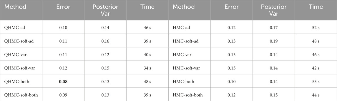
Table 1. Comparison of QHMC and HMC on 2D, inequality.
Figure 1 presents the relative error values of the algorithms with respect to two parameters: the size of the dataset and signal-to-noise ratio (SNR). It can be seen that the most accurate results without adding any noise are provided by QHMCboth and tnQHMC algorithms with around
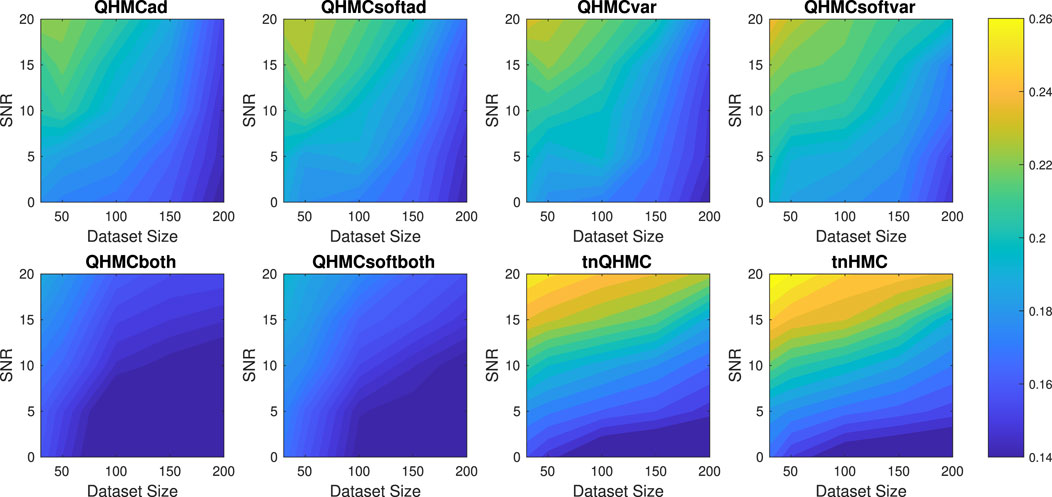
Figure 1. Relative error of the algorithms with different SNR and data sizes for Example 1 (2D), inequality.
Further, we compare the time performances of the algorithms in Figure 2 which demonstrates that QHMC methods, especially the probabilistic QHMC approaches can perform much faster than the truncated Gaussian methods. In this simple 2D problem in Equation 36, the presence of noise does not significantly impact the running times of the QHMC algorithms. In contrast, truncated Gaussian algorithms are slower under noisy environment even when the dataset size is small. Additionally, it can be observed in Figure 3 that the QHMC algorithms, especially QHMCvar and QHMCboth are the most robust ones, as their small relative error comes with a small posterior variance. In contrast, the posterior variance values of the truncated Gaussian methods are higher than QHMC posterior variances even when there is no noise, and gets higher along with the relative error (see Figure 1) when the SNR levels increase. Combining all of these experiments, the inference is that QHMC methods achieve higher accuracy within a shorter time frame. Consequently, these methods prove to be more efficient and robust as they can effectively tolerate changes in parameters. Additionally, it is worth noting that a slight improvement is achieved in the performance of truncated Gaussian algorithms by implementing tnQHMC. Based on the numerical results obtained by tnQHMC, it can be concluded that employing tnQHMC not only yields higher accuracy but also saves some computational time compared to tnHMC.
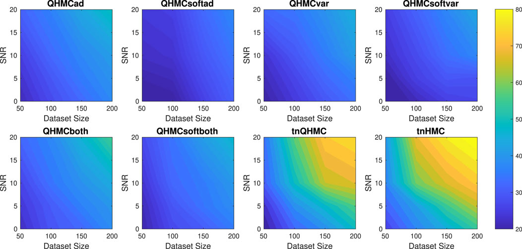
Figure 2. Execution times (in seconds) of the algorithms with different SNR and datasizes for Example 1 (2D), inequality.
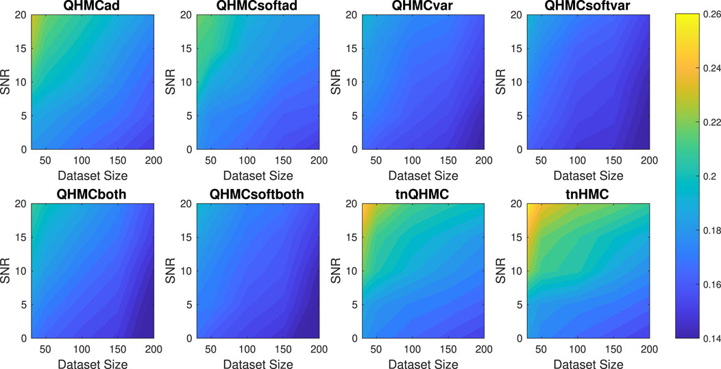
Figure 3. Posterior variances of the algorithms with different SNR and datasizes for Example 1 (2D), inequality.
4.1.2 Example 2
Consider the 10D Ackley function Eriksson and Poloczek (2021) defined as follows:
where
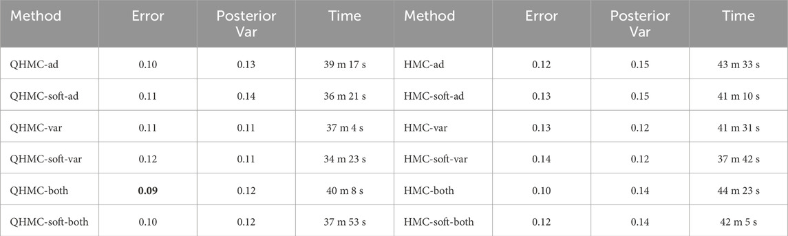
Table 2. Comparison of QHMC and HMC on 10D, inequality.
Figure 4 illustrates that QHMCboth, QHMCsoftboth and truncated Gaussian algorithms yield the lowest error when there is no noise in the data. However, as the noise level increases, truncated Gaussian methods fall behind all QHMC approaches. Specifically, both the QHMCboth and QHMCsofthboth algorithms demonstrate the ability to tolerate noise levels up to
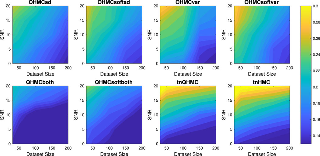
Figure 4. Relative error of the algorithms with different SNR and data sizes for Example 2 (10D), inequality.
Figure 5 illustrates the time comparison of the algorithms, where QHMC methods provide around
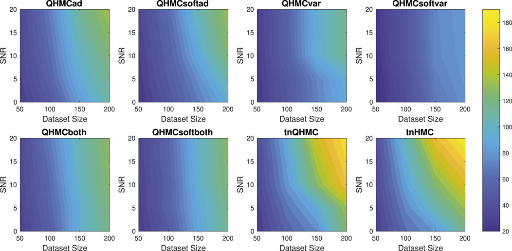
Figure 5. Execution times (in minutes) of the algorithms with different SNR and datasizes for Example 2 (10D), inequality.
Figure 6 presents that the posterior variance values of truncated Gaussian methods are significantly higher than that of the QHMC algorithms, especially when the noise levels are higher than
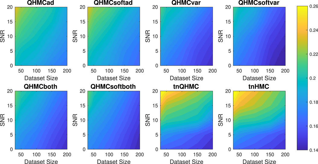
Figure 6. Posterior variances of the algorithms with different SNR and datasizes for Example 2 (10D), inequality.
4.1.3 Example 3: solute transport in heterogeneous porous media
Following the example in Yang et al. (2019), we examine conservative transport within a constant velocity field in heterogeneous porous media. Let us denote the solute concentration by
where
In this context,
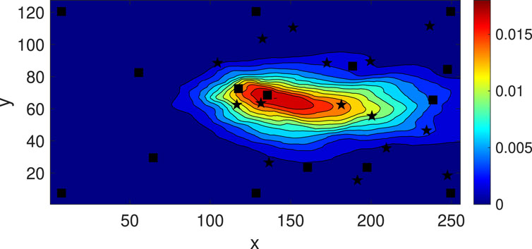
Figure 7. Observation locations (black squares) and constraint locations (black stars).
Table 3 presents a comparison of all versions of QHMC and HMC methods, along with the truncated Gaussian algorithms. Similar to the results observed with synthetic examples, the QHMCboth, QHMCsoftboth, and tnQHMC algorithms demonstrate the most accurate predictions with a relative error of
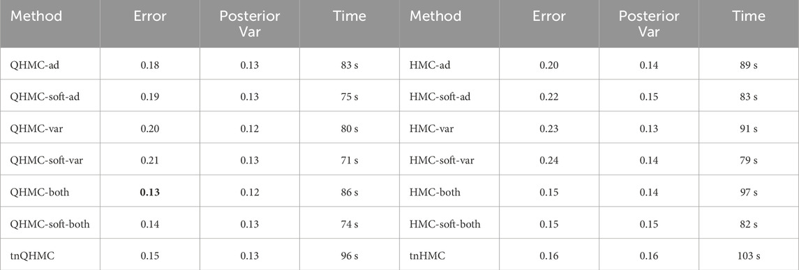
Table 3. Comparison of QHMC and HMC on solute transport with nonnegativity.
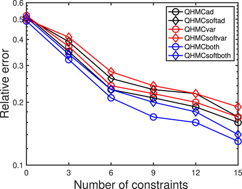
Figure 8. The change in relative error while adding constraints, solute transport.
4.1.4 Example 4: heat transfer in a hallow sphere
This 3-dimensional example considers a heat transfer problem in a hallow sphere. Let
In this context,
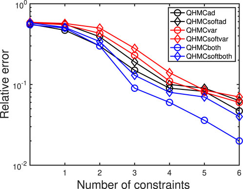
Figure 9. The change in relative error while adding constraints, heat equation.
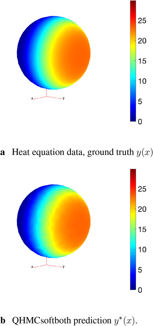
Figure 10. Comparison of the ground truth and QHMCsoftboth result. (A) Heat equation data, ground truth y(x). (B) QHMCsoftboth prediction y*(x).
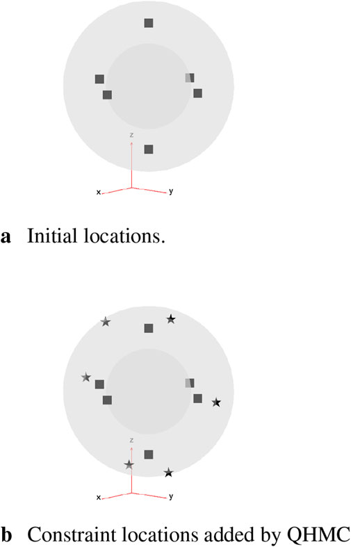
Figure 11. Initial locations (squares) and adaptively added constraint locations (stars). (A) Initial locations. (B) Constraint locations added by QHMC.
4.2 Monotonicity constraints
This section provides two numerical examples to investigate the effectiveness of our algorithms on monotonicity constraints. As stated in Section 2.3.1, the monotonicity constraints are enforced in the direction of active variables. Similar to the comparisons in previous section, we illustrate the advantages of QHMC over HMC, and then compare the performance of QHMC algorithms with additive GP approach introduced in López-Lopera et al. (2022) with respect to the same criteria as in the previous section.
4.2.1 Example 1
Consider the following 5D function with monotonicity constraints López-Lopera et al. (2022):
In this example, we enforce the function in Equation 41 to be non-decreasing with x ∈ [0, 1]^5. Table 5 shows the performances of HMC and QHMC algorithms, where we observe that QHMC achieves higher accuracy with lower variance in a shorter amount of time. The comparison proves that each version of QHMC is more efficient than HMC In addition, Figure 12 shows the relative error values of QHMC and additive GP algorithms with respect to the change in SNR and dataset size. Based on the results, it is clear that QHMCboth and QHMCsoftboth provide the most accurate results under every different condition, while the difference is more remarkable for the cases in which noise is higher. Although QHMCboth and QHMCsoftboth provides the most accurate results, other QHMC versions also generate more accurate results then additive GP method. Moreover, Figure 13 shows that the soft-constrained QHMC approaches are faster than the hard-constrained QHMC, while hard-constrained QHMC versions are still faster than additive GP algorithm. Additionally, we can see in Figure 14 that QHMC, both hard and soft constrained versions, can reduce the posterior variance. Unlike the additiveGP method, QHMC approaches generate small variances even under high noise.
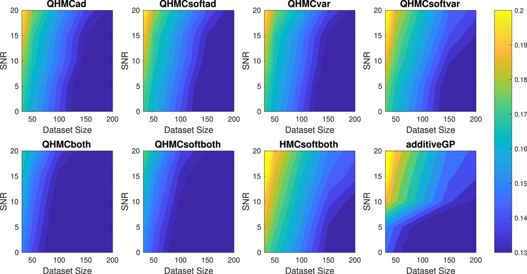
Figure 12. Relative error of the algorithms with different SNR and data sizes for Example 1 (5D), monotonicity.
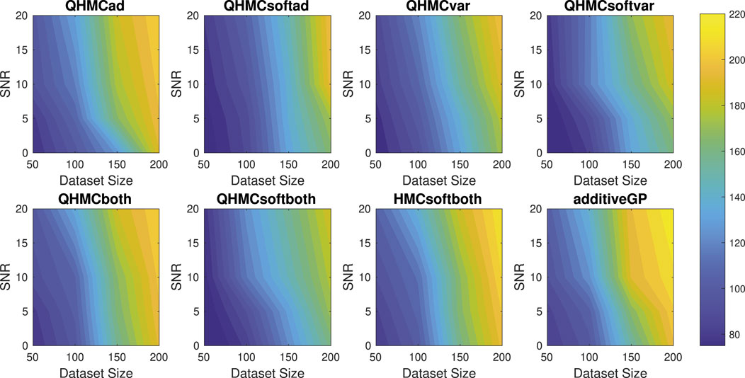
Figure 13. Execution times (in seconds) of the algorithms with different SNR and data sizes for Example 1 (5D), monotonicity.
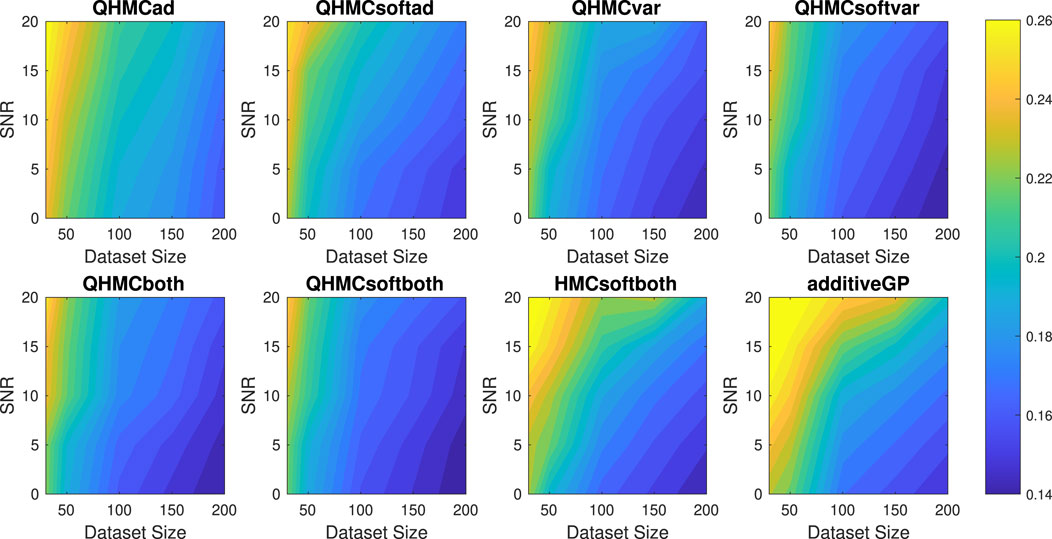
Figure 14. Posterior variances of the algorithms with different SNR and data sizes for Example 1 (5D), monotonicity.
4.2.2 Example 2
We provide a 20-dimensional example to indicate the applicability and effectiveness of QHMC algorithms on higher dimensions with monotonicity constraint. We consider the target function used in López-Lopera et al. (2022), Bachoc et al. (2022).
with
Table 6 illustrates accuracy and time advantages of QHMC over HMC. For each version of QHMC and HMC, using QHMC sampling in a specific version accelerates the process while increasing the accuracy. Overall comparison shows that among all versions with QHMC and HMC sampling, QHMCboth is the most accurate approach, while QHMCsoftboth is the fastest and ranked second in accuracy. Figures 15, 16 show the relative error and time performances of QHMC-based algorithms, HMCsoftboth and additive GP algorithm, respectively. In this final example with the highest dimension, the same phenomenon is observed as in previous results: soft-constrained versions demonstrate greater efficiency, while hard-constrained QHMC approaches remain faster than additive GP across different conditions, including high noise levels. Based on Figure 15, QHMCboth can tolerate noise levels up to
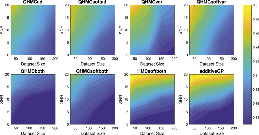
Figure 15. Relative error of the algorithms with different SNR and data sizes for Example 2 (20D), monotonicity.
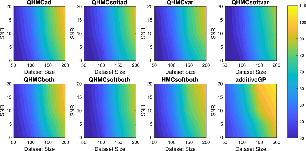
Figure 16. Execution times (in minutes) of the algorithms with different SNR and data sizes for Example 2 (20D), monotonicity.
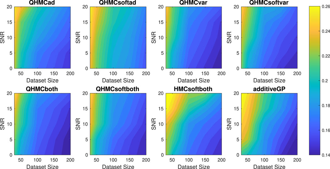
Figure 17. Posterior variances of the algorithms with different SNR and data sizes for Example 2 (20D), monotonicity.
4.3 Discussion
In the scope of the proposed QHMC-based method, this work investigates the advantages and disadvantages of using soft-constrained approach on physics-informed GP regression. The comparison of modified versions of proposed algorithm along with a recent method is further performed to validate the superiority of the approach. The significant findings and the corresponding possible reasons are summarized as follows:
1. Synthetic examples are designed to highlight the robustness and efficiency of proposed method. In one example, considering two criteria: dataset size and SNR. The QHMC-based algorithms are evaluated in an environment with a range of
2. Additionally, the numerical results of synthetic examples include the execution times for when the SNR and dataset size increase in each example. The goal is to underscore the effectiveness of the proposed algorithm. Figures 2, 5, 13, 16 show the time advantages of the algorithms, especially for the soft-constrained versions.
3. The dimensions of synthetic examples are selected to verify that the robustness and efficiency of the algorithms remain for higher dimensions. For inequality-constrained scenarios, evaluations are performed on 2D and 10D problems, while for monotonicity-constrained algorithms evaluations are performed on 5D and 20D problems. The results have verified that the performance of proposed methods can maintain the accuracy for higher-dimensional cases in a relatively short amount of times.
4. The real-life applications are chosen to verify that the proposed method is promising to generalize different type of problems. The solute concentration example is a 2D problem with non-homogeneous structure, while heat transfer problem is a 3D problem that requires PDE solving. On the contrary of synthetic examples, in this set of experiments, the dataset size is fixed and there is no injected Gaussian noise in the data. We present a comprehensive comparison of all methods along with the truncated Gaussian algorithm. Step by step decrease in the error is presented in Figures 8, 9, where the success of all versions are verified.
5. The proposed method is a combination of QHMC algorithm and a probabilistic approach for phiysics-informed GP. QHMC training provides accuracy due to its broad state space exploration, while probabilistic approach lowers the variance. In each case, we start with the experiments conducted with fixed dataset size and zero SNR to demonstrate the superiority of QHMC over HMC. The HMC versions of the proposed methods are implemented and compared to the corresponding QHMC algorithms in Tables 1, 3–6. The findings for every single case confirm that QHMC enhances the accuracy, robustness and efficiency. After demonstrating the superiority of QHMC method, a comprehensive evaluation is performed for QHMC-based methods in different scenarios. Again, for the sake of verification of efficiency of soft-constrained QHMC, we implemented the hard constrained versions by choosing the violation probability as 0.005. The findings indicate that the soft-constrained approaches reduce computational expenses while maintaining accuracy comparable to that of the hard-constrained counterparts. Releasing the constraints by a probabilistic sense has brought efficiency, while decreasing the posterior variance.
6. We should also note that while the numerical results indicate that the current approach is a robust and efficient QHMC algorithm, the impact of the probability of constraint violation should be further investigated. The experiments were conducted with a relatively low probability of releasing the constraints (around
7. While our examples demonstrate the efficiency of the proposed approach in higher dimensions (up to 20), evaluating the performance of the algorithms in much higher dimensions, such as 100 or more, remains a subject for future work. Based on the current results, we expect that the QHMC will outperform HMC, due to its sampling advantages. For example, in Liu and Zhang (2019) a stochastic version of QHMC approach is efficiently applied to train a two-layer neural network for classifying the MNIST dataset, where the weight matrices have dimensions of
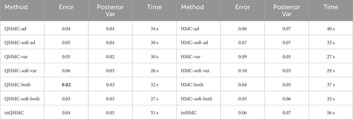
Table 4. Comparison of QHMC and HMC on heat transfer with nonnegativity.
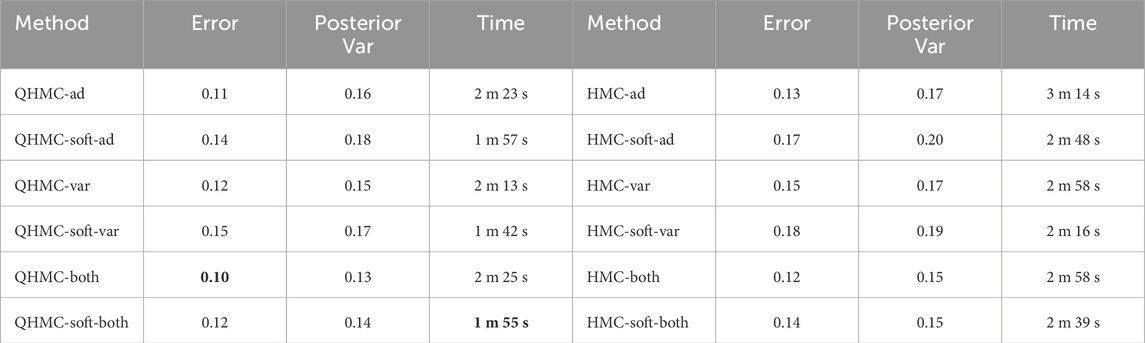
Table 5. Comparison of QHMC and HMC on 5D, monotonicity.
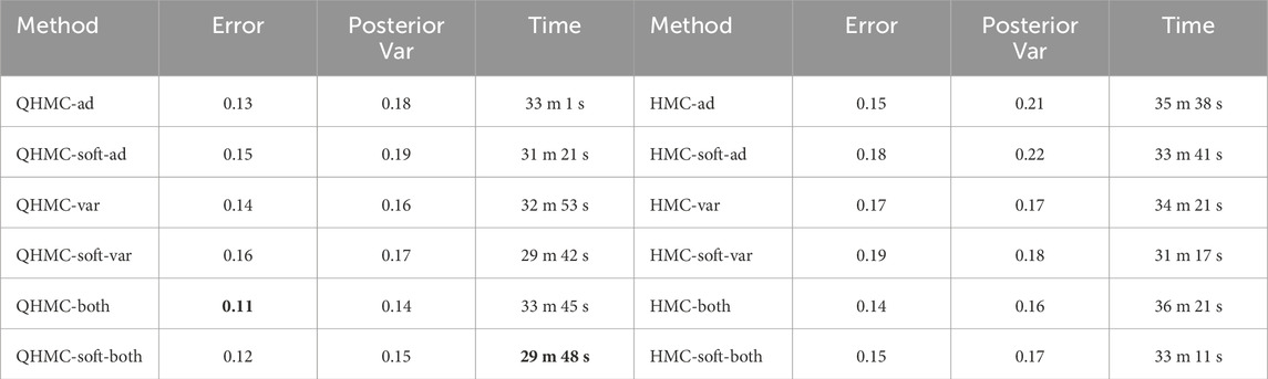
Table 6. Comparison of QHMC and HMC on 20D, monotonicity.
5 Conclusion
Leveraging the accuracy of QHMC training and the efficiency of probabilistic approach, this work introduced a soft-constrained QHMC algorithm to enforce inequality and monotonicity constraints on the GP. The proposed algorithm reduces the difference between ground truth and the posterior mean in the resulting GP model, while increasing the efficiency by attaining the accurate results in a short amount of time. To further enhance the performance of the QHMC algorithms across various scenarios, modified versions of QHMC are implemented adopting adaptive learning. These versions provide flexibility in selecting the most suitable algorithm based on the specific priorities of a given problem.
We provided the convergence of QHMC by showing that its steady-state distribution approach the true posterior density, and theoretically justified that the probabilistic approach preserves convergence. Finally, we have implemented our methods to solve several types of optimization problems. Each experiment initially outlined the benefits of QHMC sampling in comparison to HMC sampling. These advantages remained consistent across all cases, resulting in approximately a
In the context of inequality-constrained Gaussian processes (GPs), we explored 2-dimensional and 10-dimensional synthetic problems, along with two real applications involving 2-dimensional and 3-dimensional data. For synthetic examples, the relative error, posterior variance and execution time of the algorithms were compared while gradually increasing the noise level and dataset size. Overall, QHMC-based algorithms outperformed the truncated Gaussian methods. Although the truncated Gaussian methods provide high accuracy in the absence of noise and are compatible with QHMC approaches, their relative error and posterior variances increase as the noise appeared and increased. Moreover, the advantages of soft-constrained QHMC became more evident, particularly in higher-dimensional cases, when compared to truncated Gaussian and even hard-constrained QHMC. The time comparison of the algorithms underscores that the truncated Gaussian methods are significantly impacted by the curse of dimensionality and large datasets, exhibiting slower performance under these conditions. In real-world application scenarios featuring 2-dimensional and 3-dimensional data, the findings were consistent with those observed in the synthetic examples. Although the accuracy level may not reach the highest levels observed in the synthetic examples and 3-dimensional heat equation problem, the observed trend remains consistent. The lower accuracy observed in the latter problem can be attributed to the non-homogeneous structure of solute concentration.
In the case of monotonicity-constrained GP, we addressed 5-dimensional and 20-dimensional examples, utilizing the same configuration as employed for inequality-constrained GP. A comprehensive comparison was conducted between all versions of QHMC algorithms and the additive GP method. The results indicate that QHMC-based approaches hold a notable advantage, particularly in scenarios involving noise and large datasets. While additive GP proves to be a strong method suitable for high-dimensional cases, QHMC algorithms performed faster and yielded lower variances.
In conclusion, the work has demonstrated that soft-constrained QHMC is a robust, efficient and flexible method that can be applicable to higher dimensional cases and large datasets. Numerical results have shown that soft-constrained QHMC is promising to be generalized to various applications with different physical properties.
Data availability statement
The data analyzed in this study is subject to the following licenses/restrictions: Datasets are from author’s one of the previous papers. Requests to access these datasets should be directed to DK, ZGlrMzE4QGxlaGlnaC5lZHU=.
Author contributions
DK: Formal Analysis, Investigation, Methodology, Validation, Writing–original draft, Writing–review and editing. XY: Formal Analysis, Methodology, Project administration, Resources, Supervision, Writing–review and editing, Funding acquisition.
Funding
The author(s) declare that financial support was received for the research, authorship, and/or publication of this article. This work is supported by the NSF CAREER DMS-2143915.
Conflict of interest
The authors declare that the research was conducted in the absence of any commercial or financial relationships that could be construed as a potential conflict of interest.
Publisher’s note
All claims expressed in this article are solely those of the authors and do not necessarily represent those of their affiliated organizations, or those of the publisher, the editors and the reviewers. Any product that may be evaluated in this article, or claim that may be made by its manufacturer, is not guaranteed or endorsed by the publisher.
References
Abrahamsen, P., and Benth, F. E. (2001). Kriging with inequality constraints. Math. Geol. 33, 719–744. doi:10.1023/a:1011078716252
Agrell, C. (2019). Gaussian processes with linear operator inequality constraints. arXiv Prepr. arXiv:1901, 03134.
Bachoc, F., López-Lopera, A. F., and Roustant, O. (2022). Sequential construction and dimension reduction of Gaussian processes under inequality constraints. SIAM J. Math. Data Sci. 4, 772–800. doi:10.1137/21m1407513
Barbosa, B. H. G., Xu, N., Askari, H., and Khajepour, A. (2021). Lateral force prediction using Gaussian process regression for intelligent tire systems. IEEE Trans. Syst. Man, Cybern. Syst. 52, 5332–5343. doi:10.1109/tsmc.2021.3123310
Chati, Y. S., and Balakrishnan, H. (2017). “A Gaussian process regression approach to model aircraft engine fuel flow rate,” in Proceedings of the 8th international conference on cyber-physical systems, 131–140.
Da Veiga, S., and Marrel, A. (2012). Gaussian process modeling with inequality constraints. Ann. la Fac. Sci. Toulouse Mathématiques 21, 529–555. doi:10.5802/afst.1344
Dürichen, R., Pimentel, M. A., Clifton, L., Schweikard, A., and Clifton, D. A. (2014). “Multi-task Gaussian process models for biomedical applications,” in IEEE-EMBS international Conference on Biomedical and health informatics (BHI) (IEEE), 492–495.
Emmanuel, S., and Berkowitz, B. (2005). Mixing-induced precipitation and porosity evolution in porous media. Adv. water Resour. 28, 337–344. doi:10.1016/j.advwatres.2004.11.010
Eriksson, D., and Poloczek, M. (2021). Scalable constrained Bayesian optimization, In Proceedings of the 24th International Conference on Artificial Intelligence and Statistics (PMLR 130:730–738, 2021), 730–738606.
Ezati, M., Esmaeilbeigi, M., and Kamandi, A. (2024). Novel approaches for hyper-parameter tuning of physics-informed Gaussian processes: application to parametric pdes. Eng. Comput. 40, 3175–3194. doi:10.1007/s00366-024-01970-8
Gelman, A., Carlin, J. B., Stern, H. S., Dunson, D. B., Vehtari, A., and Rubin, D. B. (2014). Bayesian data analysis. Philadelphia, Pennsylvania: Tyler & Francis Group, Inc.
Gulian, M., Frankel, A., and Swiler, L. (2022). Gaussian process regression constrained by boundary value problems. Comput. Methods Appl. Mech. Eng. 388, 114117. doi:10.1016/j.cma.2021.114117
Guo, S., Xu, H., and Zhang, L. (2015). Convergence analysis for mathematical programs with distributionally robust chance constraint. SIAM J. Optim. 27, 784–816. (to appear). doi:10.1137/15m1036592
Hess, C. (1999). Conditional expectation and martingales of random sets. Pattern Recognit. 32, 1543–1567. doi:10.1016/s0031-3203(99)00020-5
Jensen, B. S., Nielsen, J. B., and Larsen, J. (2013). “Bounded Gaussian process regression,” in 2013 IEEE international workshop on machine learning for signal processing (MLSP) (IEEE), 1–6.
Kochan, D., Zhang, Z., and Yang, X. (2022). “A quantum-inspired Hamiltonian Monte Carlo method for missing data imputation,” in Mathematical and scientific machine learning (PMLR), 17–32.
Kohanpur, A. H., Saksena, S., Dey, S., Johnson, J. M., Riasi, M. S., Yeghiazarian, L., et al. (2023). Urban flood modeling: uncertainty quantification and physics-informed Gaussian processes regression forecasting. Water Resour. Res. 59, e2022WR033939. doi:10.1029/2022wr033939
Kuss, M., and Rasmussen, C. (2003). Gaussian processes in reinforcement learning. Adv. neural Inf. Process. Syst. 16.
Lange-Hegermann, M. (2021). Linearly constrained Gaussian processes with boundary conditions. In Proceedings of The 24th International Conference on Artificial Intelligence and Statistics (PMLR628 130: 1090–1098).
Li, X.-Q., Song, L.-K., Choy, Y.-S., and Bai, G.-C. (2023). Fatigue reliability analysis of aeroengine blade-disc systems using physics-informed ensemble learning. Philosophical Trans. R. Soc. A 381, 20220384. doi:10.1098/rsta.2022.0384
Lin, G., and Tartakovsky, A. M. (2009). An efficient, high-order probabilistic collocation method on sparse grids for three-dimensional flow and solute transport in randomly heterogeneous porous media. Adv. Water Resour. 32, 712–722. doi:10.1016/j.advwatres.2008.09.003
Liu, Z., and Zhang, Z. (2019). Quantum-inspired Hamiltonian Monte Carlo for bayesian sampling. arXiv Prepr. arXiv:1912.01937.
López-Lopera, A., Bachoc, F., and Roustant, O. (2022). High-dimensional additive Gaussian processes under monotonicity constraints. Adv. Neural Inf. Process. Syst. 35, 8041–8053.
López-Lopera, A. F., Bachoc, F., Durrande, N., and Roustant, O. (2018). Finite-dimensional Gaussian approximation with linear inequality constraints. SIAM/ASA J. Uncertain. Quantification 6, 1224–1255. doi:10.1137/17m1153157
Maatouk, H., and Bay, X. (2017). Gaussian process emulators for computer experiments with inequality constraints. Math. Geosci. 49, 557–582. doi:10.1007/s11004-017-9673-2
Maatouk, H., Roustant, O., and Richet, Y. (2015). Cross-validation estimations of hyper-parameters of Gaussian processes with inequality constraints. Procedia Environ. Sci. 27, 38–44. doi:10.1016/j.proenv.2015.07.105
Mao, Z., Jagtap, A. D., and Karniadakis, G. E. (2020). Physics-informed neural networks for high-speed flows. Comput. Methods Appl. Mech. Eng. 360, 112789. doi:10.1016/j.cma.2019.112789
Nabati, M., Ghorashi, S. A., and Shahbazian, R. (2022). Jgpr: a computationally efficient multi-target Gaussian process regression algorithm. Mach. Learn. 111, 1987–2010. doi:10.1007/s10994-022-06170-3
Pensoneault, A., Yang, X., and Zhu, X. (2020). Nonnegativity-enforced Gaussian process regression. Theor. Appl. Mech. Lett. 10, 182–187. doi:10.1016/j.taml.2020.01.036
Pimentel, M. A., Clifton, D. A., Clifton, L., and Tarassenko, L. (2013). “Probabilistic estimation of respiratory rate using Gaussian processes,” in 2013 35th annual international conference of the IEEE engineering in medicine and biology society (EMBC) (IEEE), 2902–2905.
Qiang, B., Shi, K., Liu, N., Ren, J., and Shi, Y. (2023). Integrating physics-informed recurrent Gaussian process regression into instance transfer for predicting tool wear in milling process. J. Manuf. Syst. 68, 42–55. doi:10.1016/j.jmsy.2023.02.019
Raissi, M., Perdikaris, P., and Karniadakis, G. E. (2017). Machine learning of linear differential equations using Gaussian processes. J. Comput. Phys. 348, 683–693. doi:10.1016/j.jcp.2017.07.050
Rasmussen, C. E., and Nickisch, H. (2010). Gaussian processes for machine learning (gpml) toolbox. J. Mach. Learn. Res. 11, 3011–3015.
Riihimäki, J., and Vehtari, A. (2010). “Gaussian processes with monotonicity information,” in Proceedings of the thirteenth international conference on artificial intelligence andf statistics (JMLR Workshop and Conference Proceedings), 645–652.
Salzmann, M., and Urtasun, R. (2010). Implicitly constrained Gaussian process regression for monocular non-rigid pose estimation. Adv. neural Inf. Process. Syst. 23.
Song, F., Shi, K., and Li, K. (2021). “A nonlinear finite element-based supervised machine learning approach for efficiently predicting collapse resistance of wireline tool housings subjected to combined loads,” in ASME International Mechanical Engineering Congress and Exposition (American Society of Mechanical Engineers). doi:10.1115/imece2021-7222285680V012T12A057
Stein, M. L. (1988). Asymptotically efficient prediction of a random field with a misspecified covariance function. Ann. Statistics 16, 55–63. doi:10.1214/aos/1176350690
Swiler, L. P., Gulian, M., Frankel, A. L., Safta, C., and Jakeman, J. D. (2020). A survey of constrained Gaussian process regression: approaches and implementation challenges. J. Mach. Learn. Model. Comput. 1, 119–156. doi:10.1615/jmachlearnmodelcomput.2020035155
Wang, Y., Wang, Z., Han, K., Tiwari, P., and Work, D. B. (2021). “Personalized adaptive cruise control via Gaussian process regression,” in 2021 IEEE international intelligent transportation systems conference (ITSC) (IEEE), 1496–1502.
Wilkie, D., and Galasso, C. (2021). Gaussian process regression for fatigue reliability analysis of offshore wind turbines. Struct. Saf. 88, 102020. doi:10.1016/j.strusafe.2020.102020
Williams, C. K., and Rasmussen, C. E. (2006). Gaussian Processes for Machine Learning 2. MA: MIT press Cambridge.
Yang, X., Barajas-Solano, D., Tartakovsky, G., and Tartakovsky, A. M. (2019). Physics-informed cokriging: a Gaussian-process-regression-based multifidelity method for data-model convergence. J. Comput. Phys. 395, 410–431. doi:10.1016/j.jcp.2019.06.041
Yang, X., Tartakovsky, G., and Tartakovsky, A. M. (2021). Physics information aided kriging using stochastic simulation models. SIAM J. Sci. Comput. 43, A3862–A3891. doi:10.1137/20m1331585
Zhang, H. (2004). Inconsistent estimation and asymptotically equal interpolations in model-based geostatistics. J. Am. Stat. Assoc. 99, 250–261. doi:10.1198/016214504000000241
Nomenclature
Abbreviations
additiveGP Additive Gaussian Process method
GP Gaussian Process
HMC Hamiltonian Monte Carlo
HMCad Hard-constrained Hamiltonian Monte Carlo with adaptivity
HMCboth Hard-constrained Hamiltonian Monte Carlo with both adaptivity and variance
HMCsoftad Soft-constrained Hamiltonian Monte Carlo with adaptivity
HMCsoftboth Soft-constrained Hamiltonian Monte Carlo with both adaptivity and variance
HMCsoftvar Soft-constrained Hamiltonian Monte Carlo with variance
HMCvar Hard-constrained Hamiltonian Monte Carlo with variance
MCMC Markov chain Monte Carlo
MH Metropolis-Hastings
PDE Partial differential equations
QHMC Quantum-inspired Hamiltonian Monte Carlo
QHMCad Hard-constrained Quantum-inspired Hamiltonian Monte Carlo with adaptivity
QHMCboth Hard-constrained Quantum-inspired Hamiltonian Monte Carlo with adaptivity and variance
QHMCsoftad Soft-constrained Quantum-inspired Hamiltonian Monte Carlo with adaptivity
QHMCsoftboth Soft-constrained Quantum-inspired Hamiltonian Monte Carlo with both adaptivity and variance
QHMCsoftvar Soft-constrained Quantum-inspired Hamiltonian Monte Carlo with variance
QHMCvar Hard-constrained Quantum-inspired Hamiltonian Monte Carlo with variance
SNR Signal-to-noise ratio
tnHMC Truncated Gaussian method with Hamiltonian Monte Carlo sampling
tnQHMC Truncated Gaussian method with Quantum-inspired Hamiltonian Monte Carlo sampling
Symbols
Keywords: constrained optimization, Gaussian process regression, quantum-inspired Hamiltonian Monte Carlo, adaptive learning, soft constraints
Citation: Kochan D and Yang X (2025) Blending physics with data using an efficient Gaussian process regression with soft inequality and monotonicity constraints. Front. Mech. Eng. 10:1410190. doi: 10.3389/fmech.2024.1410190
Received: 31 March 2024; Accepted: 23 December 2024;
Published: 23 January 2025.
Edited by:
Ke Li, Schlumberger, United StatesReviewed by:
Lu-Kai Song, Beihang University, ChinaXueyu Zhu, The University of Iowa, United States
Fei Song, Schlumberger, United States
Copyright © 2025 Kochan and Yang. This is an open-access article distributed under the terms of the Creative Commons Attribution License (CC BY). The use, distribution or reproduction in other forums is permitted, provided the original author(s) and the copyright owner(s) are credited and that the original publication in this journal is cited, in accordance with accepted academic practice. No use, distribution or reproduction is permitted which does not comply with these terms.
*Correspondence: Xiu Yang, eGl5NTE4QGxlaGlnaC5lZHU=