Simulations of decane-ammonia autoignition in two mixture fractions

This paper presents a zero-dimensional Doubly Conditional Moment Closure (0D-DCMC) methodology for investigating dual-fuel combustion involving ammonia and diesel. The approach uses two mixture fractions as conditioning variables, one for each fuel, to effectively model ignition and reveal the flame structure in mixture fraction space. Initially, 0D reactor calculations are performed using Cantera, exploring the chemical mechanism, identifying the most reactive mixture fractions, and determining key species involved in the ignition process. Following that, the 0D-DCMC simulations carried out provide understanding into the effects of the scalar and cross-scalar dissipation rates on autoignition. The results show that higher scalar dissipation rates delay ignition, while a negative cross-scalar dissipation rate reduces ignition delay compared to a positive rate. The ignition is shown to occur near the most reactive mixture fraction of the most reactive fuel, at lower conditional values of the less reactive fuel’s mixture fraction. The species fronts formed are observed to follow a trajectory between the stoichiometric mixture fractions of the fuels. The results establish a robust computational framework for modeling dual-fuel combustion.

1 Introduction

Following the Paris Agreement in 2015 (UNFCCC, 2024), the International Maritime Organisation is aiming at 50% greenhouse gas emissions reduction compared to 2008 by 2050 (Joung et al., 2020). Shipping is responsible for carrying around 80% of global trade by volume (United Nations, 2018) producing however an estimated 2.2% of global emissions ${\text{CO}}_2$ (International Maritime Organization, 2015). With increasing environmental regulations and mounting concerns about greenhouse gas emissions (Simon et al., 2020), the search for cleaner alternative fuels has become imperative (Chin et al., 2021). Ammonia has emerged as a promising candidate due to its carbon-free nature (Ramanathan et al., 2023) and the potential to significantly reduce marine pollution (Wong et al., 2024). Due to its zero carbon and sulfur content, burning NH3 in an engine results in almost no ${\text{CO}}_2$ or ${\text{SO}}_X$ emissions with potential for reducing GHG by 94% (Zhou et al., 2024). From a well-to-wake standpoint, ammonia is a carbon-neutral fuel when it is generated using renewable energy sources (MAN Energy Solutions, 2023). The elimination of pollutants also includes soot, unburned hydrocarbons, methane slip, and CO.

However, ammonia is a difficult fuel to burn. The flame speed is low and its ignition time long (Valera-Medina et al., 2018), which necessitates special measures to consume it successfully. One such approach is dual-fuel combustion and in particular pilot ignition, where an easy-to-ignite hydrocarbon fuel is injected into the cylinder first, so that its ignition provides a distributed ignition source for the ammonia. Reciprocating engines are expected to be one the key technologies for using ammonia in shipping in the future (Curran et al., 2024). If the ammonia is already premixed with air, then an ammonia premixed flame will initiate, but if the ammonia is injected separately as in a direct injection concept, there will be a non-premixed ammonia-air system that must be ignited. This paper deals with the latter possibility and provides some fundamental understanding of the underlying chemistry and how this is affected by diffusion.

Revealing the fundamental effects of simultaneous mixing and chemical reaction is often done by resort to the mixture fraction, as in the flamelet method [for a review, see the textbooks (Poinsot and Veynante, 2005; Peters, 2001)]. In our dual-fuel case, however, we need two mixture fractions. In the current analysis, the Doubly Conditional Moment Closure method presented by Sitte and Mastorakos (Philip, 2019) is extended to a two-mixture fraction approach. There have been previous efforts in 2D flamelet calculations using the two mixture fraction approach in staged combustion (secondary oxidizer stream) (Perry et al., 2017; Yu and Watanabe, 2023) accurately capturing the flame structure of the combustion system, but there have not been explorations of flame structures in mixture fraction space for hydrocarbon-ammonia systems. Here, the general features of hydrocarbon ignition will be mimicked by decane, for which detailed chemistry is available.

The objectives of this paper are to study decane-ammonia combustion systems, and in particular decane autoignition and the subsequent ignition of the ammonia-air flame, through a Doubly-Conditional Moment Closure formulation. The structure of the flames is explored and the sensitivity to scalar dissipation quantified.

2 Numerical methods

2.1 Flamelet and CMC

In the standard flamelet approach, the functions T ($\xi$, t), $Y_k(\xi ,t)$ define the flame structure if we assume that the structure of the diffusion flame depends only on the mixture fraction $\xi$ and on time $t$. This is substantiated by making a variable change in the species equations from (${\text{x}}_1$, ${\text{x}}_2$, ${\text{x}}_3$, t) to (z, ${\text{y}}_2$, ${\text{y}}_3$, t) where ${\text{y}}_2$ and ${\text{y}}_3$ are spatial variables in planes parallel to iso-$\xi$ surfaces (Poinsot and Veynante, 2005).

$T=T\left(\xi ,t\right)and{Y}_K=Y_k\left(\xi ,t\right)(1)$

Neglecting the terms associated with gradients along the flame front (${\text{y}}_2$ and ${\text{y}}_3$) and keeping the terms perpendicular to the flame (along $\xi$) as significant we could approximate the flame structure locally as one-dimensional, depending only on time and the coordinate normal to the flame front $(\xi )$ as presented in Equation 1. For this assumption to hold the flame must be thin compared to other flow and wrinkling scales in a multi-dimensional flow (Poinsot and Veynante, 2005). This implies that each part of the flame front can be approximated as a small laminar flame, the “flamelet”. Following the above the species mass fraction equation as well as the temperature are written as follows in Equations 2, 3:

$\rho \frac{\partial Y_k}{\partial t}={\dot{\omega }}_k+\frac{1}{2}\rho \chi \frac{{\partial }^2{Y}_k}{\partial {\xi }^2}(2)$

$\rho \frac{\partial T_k}{\partial t}={\dot{\omega }}_T+\frac{1}{2}\rho \chi \frac{{\partial }^{2}T}{\partial {\xi }^2}(3)$

The only term depending on spatial variables (${\text{x}}_i$), in the flamelet Equations 2, 3 is the scalar dissipation rate $\chi$ which controls mixing as it dictates the gradients of $\xi$ (Poinsot and Veynante, 2005). Once $\chi$ is specified, Equations 2, 3 can be solved in the $\xi$ space to provide the flame structure. The usual way to determine its value/distribution is by performing a direct numerical simulation of the problem under consideration or an experiment. If this is not the case, a try error process is followed in order to allocate what is called the extinction scalar dissipation rate over which the flame cannot exist.

The flamelet equations can also be understood as a subset of the Conditional Moment Closure approach, reviewed in Bilger (1993), where the conditioning is performed based on the mixture fraction (Peters, 2001). Rather than focusing on flame surface statistics and the laminar reactive-diffusive structure tied to the flame surface as is the case in the flamelet model, CMC employs conditional moments at a particular location x and time t within the flow field, using the conditional probability density function (Peters, 2001). The flame structure is characterized by the conditional averages of the reactive scalars and the conditional mean $Q_a$ is defined as the ensemble average of $Y_a(x,t)$ under the condition that the associated value $\xi (x,t)$ is at the value $\eta$ (Philip, 2019) as seen in Equation 4:

$Q_{\alpha }\left(\eta ;x,t\right)\equiv \langle Y_{\alpha }\left(x,t\right)\mid \xi \left(x,t\right)=\eta \rangle \equiv \langle Y_{\alpha }\mid \eta \rangle (4)$

Through this averaging process, the instantaneous reactive scalar value can be recovered into the conditional mean and a deviation from the conditional mean as presented in Equation 5 (Bilger, 1993):

$Y_{\alpha }\left(x,t\right)=Q_{\alpha }\left(\xi \left(x,t\right);x,t\right)+{Y^{″}}_{\alpha }\left(x,t\right)(5)$

The core concept of the CMC method involves solving transport equations for the conditional averages of reactive scalars in order to determine the flame structure (Philip, 2019). Furthermore, an exact transport equation for these conditional moments can be derived. That is by adopting a set of assumptions, including high Reynolds number, the primary closure hypothesis, molecular-level Fickian mass diffusion, a Lewis number of unity, and negligible conditional density fluctuations, the equation can be simplified to the form of Equation 6 (Klimenko and Bilger, 1999):

$\frac{\partial Q_{\alpha }}{\partial t}+\langle u\mid \eta \rangle \cdot \nabla Q_{\alpha }=\langle N_{\xi }\mid \eta \rangle \frac{{\partial }^2{Q}_{\alpha }}{\partial {\eta }^2}+\langle {\dot{\omega }}_{\alpha }\mid \eta \rangle -\frac{\nabla \cdot \left(\langle \rho \mid \eta \rangle \langle u^{″}{Y^{″}}_{\alpha }\mid \eta \rangle p\left(\eta \right)\right)}{\langle \rho \mid \eta \rangle p\left(\eta \right)}(6)$

The unconditional mean of a variable can be determined from its conditional means as follows:

$⟨Y_{\alpha }\left(x,t\right)⟩={\int }_0^1{Q}_{\alpha }\left(\eta ;x,t\right)p\left(\eta ;x,t\right)d\eta (7)$

2.2 DCMC equations

The DCMC equations presented in this sub-section are adapted from the work of Philip (2019). The rationale for using double conditioning is that if most fluctuations around the single-conditional mean can be linked to the second conditional variable, then the fluctuations around the double-conditional mean, determined by two mixture fractions, should be small (Philip, 2019). As singly-conditioned CMC models are limited to cases that are either premixed or predominantly non-premixed (Philip Sitte and Mastorakos, 2019) the double conditioning allows for a wider description of phenomena present in dual fuel systems. The DCMC method extends the parameter space and incorporates the cross-scalar dissipation rate, while remaining a straightforward generalization of the CMC approach. Additionally, it is expected to describe well all combustion modes relevant to dual-fuel engines (Harikrishnan et al., 2024). The doubly conditional space is as follows in Equation 8:

$D=\left\{\left({\eta }_1,{\eta }_2\right)\in {\mathbb{R}}^2:0\le {\eta }_1\le 1,0\le {\eta }_2\le 1\right\}(8)$

The conditional mass fractions are given in Equation 9 and the conditional enthalpy in Equation 10. The conditional temperature equation also exists but only one of the temperature and enthalpy need to be solved choosing the latter:

$\begin{array}{cc}\hfill & \frac{\partial Q_{\alpha }}{\partial t}+\nabla \cdot \left(Q_{\alpha }\langle \mathbf{u}\mid {\eta }_1,{\eta }_2\rangle \right)=Q_{\alpha }\nabla \cdot \left(\langle \mathbf{u}\mid {\eta }_1,{\eta }_2\rangle \right)\hfill \\ \hfill & -\frac{1}{\bar{\rho }\tilde{p}}\nabla \cdot \left(\bar{\rho }\tilde{p}\left[\langle \mathbf{u}{Y}_{\alpha }\mid {\eta }_1,{\eta }_2\rangle -Q_{\alpha }\langle \mathbf{u}\mid {\eta }_1,{\eta }_2\rangle \right]\right)\hfill \\ \hfill & +\frac{1}{\bar{\rho }\tilde{p}}\nabla \cdot \left(\bar{\rho }\tilde{p}\langle D\nabla Y_{\alpha }\mid {\eta }_1,{\eta }_2\rangle \right)\hfill \\ \hfill & +\langle N_{{\xi }_1}\mid {\eta }_1,{\eta }_2\rangle \frac{{\partial }^2{Q}_{\alpha }}{\partial {\eta }_1^2}+2\langle N_{{\xi }_1{\xi }_2}\mid {\eta }_1,{\eta }_2\rangle \frac{{\partial }^2{Q}_{\alpha }}{\partial {\eta }_1\partial {\eta }_2}\hfill \\ \hfill & +\langle N_{{\xi }_2}\mid {\eta }_1,{\eta }_2\rangle \frac{{\partial }^2{Q}_{\alpha }}{\partial {\eta }_2^2}+\langle {\dot{\omega }}_{\alpha }\mid {\eta }_1,{\eta }_2\rangle \hfill \\ \hfill & -\langle {\dot{\omega }}_c^{*}\mid {\eta }_1,{\eta }_2\rangle \frac{\partial Q_{\alpha }}{\partial {\eta }_2}\hfill \end{array}(9)$

$\begin{array}{cc}\hfill & \frac{\partial Q_h}{\partial t}+\nabla \cdot \left(Q_h\langle u\mid {\eta }_1,{\eta }_2\rangle \right)=Q_h\nabla \cdot \left(\langle u\mid {\eta }_1,{\eta }_2\rangle \right)\hfill \\ \hfill & -\frac{1}{\bar{\rho }\tilde{p}}\nabla \cdot \left(\bar{\rho }\tilde{p}\left[\langle uh\mid {\eta }_1,{\eta }_2\rangle -Q_h\langle u\mid {\eta }_1,{\eta }_2\rangle \right]\right)\hfill \\ \hfill & +\frac{1}{\bar{\rho }\tilde{p}}\nabla \cdot \left(\bar{\rho }\tilde{p}\langle a\nabla h\mid {\eta }_1,{\eta }_2\rangle \right)\hfill \\ \hfill & +\langle N_{{\xi }_1}\mid {\eta }_1,{\eta }_2\rangle \frac{{\partial }^2{Q}_h}{\partial {\eta }_1^2}+2\langle N_{{\xi }_1{\xi }_2}\mid {\eta }_1,{\eta }_2\rangle \frac{{\partial }^2{Q}_h}{\partial {\eta }_1\partial {\eta }_2}\hfill \\ \hfill & +\langle N_{{\xi }_2}\mid {\eta }_1,{\eta }_2\rangle \frac{{\partial }^2{Q}_h}{\partial {\eta }_2^2}\hfill \\ \hfill & -\langle {\dot{\omega }}_c^{*}\mid {\eta }_1,{\eta }_2\rangle \frac{\partial Q_h}{\partial {\eta }_2}+〈\frac{1}{\rho }no\frac{\partial p}{\partial t}n|e{\eta }_{1}e,e{\eta }_2〉\hfill \end{array}(10)$

where, according to Harikrishnan et al. (2024), the following are true: $⟨N_{{\xi }_1}\mid {\eta }_1,{\eta }_2⟩$, $⟨N_{{\xi }_2}\mid {\eta }_1,{\eta }_2⟩$, and $⟨N_{{\xi }_1{\xi }_2}\mid {\eta }_1,{\eta }_2⟩$ are the conditional scalar dissipation rates (SDRs) of ${\xi }_1$, ${\xi }_2$, and the cross-scalar dissipation rate, respectively. The final term in the $Q_h$ equation accounts for the pressure $(p)$ rise in the constant volume chamber. The term $⟨{\dot{\omega }}_{\alpha }\mid {\eta }_1,{\eta }_2⟩$ represents the conditional chemical source term while the $⟨u\mid {\eta }_1,{\eta }_2⟩$, $\tilde{p}$, and $\bar{\rho }$ are the conditional velocity, Favre-filtered probability density function, and filtered density, respectively. Moving on, ${\eta }_1$ and ${\eta }_2$ are the respective sample space variables for the two mixture fractions. Finally, $⟨{\dot{\omega }}_c^{*}\mid {\eta }_1,{\eta }_2⟩$ is the conditional apparent reaction rate term. The apparent reaction rate, encapsulating both the direct chemical source term and effects of the effects of the scalar dissipation rates, is presented in Equation 11:

$\begin{array}{cc}\hfill ⟨{\dot{\omega }}_c^{*}\mid {\eta }_1,{\eta }_2⟩& =\frac{1}{\frac{\partial Q_{\psi }}{\partial {\eta }_2}}\left[⟨{\dot{\omega }}_{\psi }\mid {\eta }_1,{\eta }_2⟩+⟨N_{{\xi }_1}\mid {\eta }_1,{\eta }_2⟩\frac{{\partial }^2{Q}_{\psi }}{\partial {\eta }_1^2}\right.\hfill \\ \hfill & \left.+2⟨N_{{\xi }_1{\xi }_2}\mid {\eta }_1,{\eta }_2⟩\frac{{\partial }^2{Q}_{\psi }}{\partial {\eta }_1\partial {\eta }_2}+⟨N_{{\xi }_2}\mid {\eta }_1,{\eta }_2⟩\frac{{\partial }^2{Q}_{\psi }}{\partial {\eta }_2^2}\right]\hfill \end{array}(11)$

The conditional expectation of the mixture fraction SDR, $⟨N_{\xi }\mid {\eta }_1,{\eta }_2⟩$, presented in Equation 12 is modeled using Amplitude Mapping Closure (AMC) (O’Brien and Jiang, 1991) of Equation 13. The shape of this bell curve plays a significant role in the diffusion in mixture fraction space due to the zero value it assumes at the boundaries not allowing diffusion to those points from internal values of the mixture fraction.

$⟨N_{\xi }\mid {\eta }_1,{\eta }_2⟩=N_0{G}_{\xi }\left({\eta }_1\right)(12)$

where,

$G_{\xi }\left(\eta \right)=\exp \left(-2{\left({erf}^{-1}\left(2\eta -1\right)\right)}^2\right)(13)$

$N_0=\frac{{\tilde{N}}_{\xi }}{{\int }_0^1{\int }_0^1{G}_{\xi }\left({\eta }_1\right)\tilde{p}\left({\eta }_1,{\eta }_2\right)d{\eta }_{1}d{\eta }_2}(14)$

$N_{{\xi }_1}\equiv D\nabla {\xi }_1\cdot \nabla {\xi }_1,N_{{\xi }_2}\equiv D\nabla {\xi }_2\cdot \nabla {\xi }_2,N_{{\xi }_1{\xi }_2}\equiv D\nabla {\xi }_1\cdot \nabla {\xi }_2(15)$

where $N_0=⟨N_{\xi }\mid 0.5,{\eta }_2⟩$ and $⟨N_{\xi }\mid {\eta }_1,0.5⟩$ respectively using Equation 14. The modeling of the cross-scalar dissipation rate is still a matter of research and constitutes a central input to the DCMC method. The modelling of the latter term of Equation 15 is proposed in Equation 16 by Kronenburg (2004) is utilized.

$⟨N_{{\xi }_1{\xi }_2}\mid {\eta }_1,{\eta }_2⟩=\frac{\sqrt{{\tilde{N}}_{{\xi }_1{\xi }_2}}}{\sqrt{{\tilde{N}}_{{\xi }_1}{\tilde{N}}_{{\xi }_2}}}\sqrt{⟨N_{{\xi }_1}\mid {\eta }_1,{\eta }_2⟩}\sqrt{⟨N_{{\xi }_2}\mid {\eta }_1,{\eta }_2⟩}(16)$

The ratio $\frac{\sqrt{{\tilde{N}}_{{\xi }_1{\xi }_2}}}{\sqrt{{\tilde{N}}_{{\xi }_1}{\tilde{N}}_{{\xi }_2}}}$ will be denoted by $N_{\mathit{rat}}$ in this paper and its magnitude will be varied to examine the consequences to the solution. For partially premixed combustion, the cross-scalar dissipation rate is an important quantity and assumes a positive value for premixed combustion and a negative for non-premixed combustion (Chakraborty et al., 2007). There is very little information in the literature for this quantity whose modelling is a topic for further research.

2.3 0D-DCMC equations

To initially explore flame structures in dual-fuel systems, as in this paper, a simplification process is followed reducing the DCMC equations to zero dimension and essentially going from three spatial and two mixture fraction dimensions to only two mixture fraction dimensions. The underlying assumptions of the 0D-CMC equations are.

$•$ High Reynolds number that allows for the neglect of some molecular transport terms.

$•$ Unity Lewis number meaning that all reacting scalars diffuse at the same rate with the mixture fraction.

$•$ No transport in physical space, meaning that terms related to physical coordinates do not appear in the equations.

$•$ No heat losses.

$•$ Constant pressure.

$•$ Fixed $\eta$ boundaries and Dirichlet boundary conditions for $\eta =0$ and $\eta =1$.

$•$ Presumed $N\mid \eta$ profiles.

Under these assumptions, the 0D-DCMC equations assume the form of Equations 17, 18.

$\begin{array}{cc}\hfill & \frac{\partial Q_{\alpha }}{\partial t}=\langle N_{{\xi }_1}\mid {\eta }_1,{\eta }_2\rangle \frac{{\partial }^2{Q}_{\alpha }}{\partial {\eta }_1^2}+2\langle N_{{\xi }_1{\xi }_2}\mid {\eta }_1,{\eta }_2\rangle \frac{{\partial }^2{Q}_{\alpha }}{\partial {\eta }_1\partial {\eta }_2}\hfill \\ \hfill & +\langle N_{{\xi }_2}\mid {\eta }_1,{\eta }_2\rangle \frac{{\partial }^2{Q}_{\alpha }}{\partial {\eta }_2^2}+\langle {\dot{\omega }}_{\alpha }\mid {\eta }_1,{\eta }_2\rangle \hfill \end{array}(17)$

$\begin{array}{cc}\hfill & \frac{\partial Q_h}{\partial t}=\langle N_{{\xi }_1}\mid {\eta }_1,{\eta }_2\rangle \frac{{\partial }^2{Q}_h}{\partial {\eta }_1^2}+2\langle N_{{\xi }_1{\xi }_2}\mid {\eta }_1,{\eta }_2\rangle \frac{{\partial }^2{Q}_h}{\partial {\eta }_1\partial {\eta }_2}\hfill \\ \hfill & +\langle N_{{\xi }_2}\mid {\eta }_1,{\eta }_2\rangle \frac{{\partial }^2{Q}_h}{\partial {\eta }_2^2}+\langle \dot{Q}\mid {\eta }_1,{\eta }_2\rangle \hfill \end{array}(18)$

In this paper, 0D-DCMC simulations will be performed to understand the basic structure of dual-fuel autoignition systems, as a first step in a full implementation in a turbulent reacting flow multi-dimensional simulation.

2.4 Initial conditions

In this section, the initial conditions of the solution of the equations are discussed. Two mixture fractions are used, one for each fuel, ${\xi }_1$ for decane, and ${\xi }_2$ for ammonia. The initial conditions are chosen as mixing lines. These lines correspond to states where the fuel and oxidizer mix without reacting. Such mixing lines are crucial in capturing ignition and quenching (Poinsot and Veynante, 2005).

With the presence of two fuels, it is not clear what to do in the top right corner. The points $({\eta }_1,{\eta }_2)=(\mathrm{0,1})$ and $({\eta }_1,{\eta }_2)=(\mathrm{1,0})$ correspond to pure ammonia and pure diesel respectively whereas the point $({\eta }_1,{\eta }_2)=(\mathrm{0,0})$ to the pure oxidizer (air). The point $({\eta }_1,{\eta }_2)=(\mathrm{1,1})$ is a matter of debate as there are multiple options and it is unclear whether this results in different results. As we have two fuels the logical boundary condition is to consider that at that point 50$\%$ ammonia and 50$\%$ diesel (by mass) are present corresponding to a mixture. The resulting distributions are seen in Figures 1, 2. One could also set this point as 100 $\%$ ammonia or diesel altering the mathematical formulation of the problem and thus the results. However, the quantitative analysis yields the same conclusions. In conclusion, the current choice is a matter of modelling and is not expected to affect the results if the interpretation is done correctly considering the initial conditions.

Figure 1

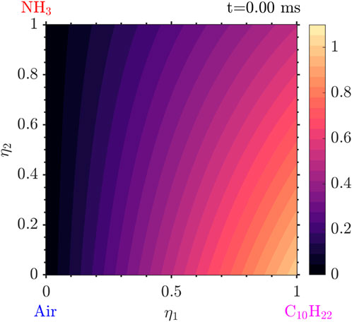
Figure 1. Initial decane mass fraction in ${\eta }_1-{\eta }_2$ space.

Figure 2

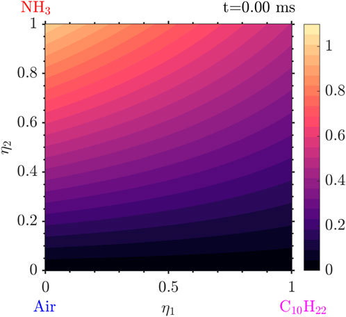
Figure 2. Initial ammonia mass fraction in ${\eta }_1-{\eta }_2$ space.

As the chemistry is detailed and the ${\text{c}}_p$ of each species is different, the initial distributions of species mass fractions and the enthalpy are linear functions of ${\xi }_1$ and ${\xi }_2$. However, the temperature is not. In the current analysis, the mass fractions and the enthalpy are used and the temperature distribution is computed from the enthalpy. The same typical approach as in the single mixture fraction case is followed for constructing the mixing lines in each of the four boundaries interpolating between the extreme values at the two corners corresponding to each boundary. The values at the inner nodes are computed from a multivariate interpolation.

2.5 Numerical procedure

The 0D-DCMC equation is a parabolic PDE in two dimensions (the two mixture fractions) and time. In a full 3D simulation in the future, we would add the 3 spatial dimensions, as in Philip, (2019), but this is not done here. The mixture fraction spaces are discretised with a 71 x 71 nonuniform grid covering the whole range of 0–1. The choice of its size is dictated by the trade-off between accuracy and computational effort. The grid is denser around the stoichiometric mixture fraction of each fuel as the flame and most reactions are expected to lie there. Due to the steep gradients and the rapid construction and destruction of species around stoichiometry, a very dense grid is required around there for accuracy. As a result, using a non-uniform grid allows for significant computational improvements. The diffusion in mixture fraction space is solved first with the VODPK solver (Alan, 1983), using the non-stiff Adam’s method which solves the set of non-linear ODEs. Central-differencing schemes for non-uniform grids, which are second-order accurate, are used for the numerical discretisation of the $\frac{{\partial }^{2}Q}{\partial {\xi }^2}$ terms.

Chemical source terms are addressed last using the SpeedCHEM solver (Perini et al., 2012). This solver, referred to as LIBSC, utilizes a sparse Jacobian formulation and precomputed, temperature-dependent properties to greatly enhance computational speed. It also supports the use of an analytical Jacobian, which approximates the Jacobian matrix of the ODE system. For most chemical mechanisms, this approach offers significant performance enhancements. Timesteps equal or smaller than ${10}^{-6}$ s are used to minimise operator splitting errors.

2.6 Chemical mechanism

This section briefly discusses the selection of the chemical mechanism used for the simulations. Typically, the physical properties of diesel, such as density and evaporation rate, are modeled using decane or dodecane, while heptane is used to mimic diesel’s chemistry. Most current chemical mechanisms for ammonia/hydrocarbon fuels are derived by merging databases for each fuel and as a result in general further research is required in this area.

A recently published chemical scheme, the Aalto75 model (Tolga Kurumus et al., 2024), includes 75 species and 451 reactions and is reported to be well-validated across various experimental datasets, including ignition delay times, laminar flame speeds, and species profiles. However, it was not used in this study as it was released after the project had already begun and is left for future work. Another chemical mechanism for ammonia/n-heptane mixtures was published by (Thorsen et al., 2023), offering good predictions of ignition delay times at pressures up to 100 bar. However, this mechanism was not selected due to its complexity, as it has too many species and reactions, making it very difficult to handle computationally for the current project.

The chemical mechanism ultimately chosen for this study is the one provided by Lin Tay et al. (2017) for decane-ammonia combustion, consisting of 80 species and 374 reactions. The ignition delay times for diesel and ammonia were found to be very similar with the parent mechanisms, indicating that this mechanism is sufficiently robust for use in diesel engine simulations and should contain the key aspects of the problem.

3 Results and discussion

3.1 0D reactor evaluation

In this section, homogeneous reactor calculations with the use of Cantera are performed. The motivation is twofold: to validate that the chemical mechanism produces reasonable results for homogeneous mixtures and to locate the “most reactive” mixture fraction ${\xi }_{mr}$ (Mastorakos, 2009) in the case of fuel-air mixing layers. For such cases, the initial condition of temperature is connected with the initial mass fractions through Equations 19–22:

$Y_{fu}=\xi \times Y_{f{u}_0}(19)$

$Y_{O_2}=\left(1-\xi \right)\times Y_{O_{2_0}}(20)$

$Y_{N_2}=\left(1-\xi \right)\times Y_{N_{2_0}}(21)$

$T=T_{ox}-\xi \times \left(T_{ox}-T_{fu}\right)(22)$

The temperature of the oxidizer is left as a parameter and the fuel temperature is set constant to 300 K. The calculations are based on a series of batch reactors for the different temperatures and pressures with the mixture fraction being varied with the initial condition as above. For each temperature or pressure, the most reactive mixture fraction is the one producing the smallest ignition delay.

A typical batch reactor simulation for the ignition of homogeneous ammonia/air mixtures is presented in Figure 3 for an oxidiser temperature of 1200 K and a pressure of 2 atm and it is found that ignition takes place at approximately 1.1 ms. We notice that the rapid temperature increase is correlated with the rise of the species OH and ${\text{H}}_2$ and that ${\text{N}}_2$O is rapidly produced and destroyed making it a pre-ignition species, as seen in the right axis of the mass fractions. ${\text{N}}_2$O, HNO, NO and ${\text{NH}}_2$ are quickly produced at the autoignition instant and then quickly destroyed. On the contrary, species like NNH and OH, although again rapidly produced, stay relatively constant after the ignition. Finally, observing the early chemistry we see that ${\text{NO}}_2$ is produced during the species accumulation period and flattens during the autoignition.

Figure 3

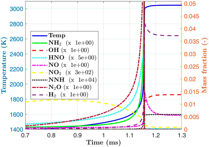
Figure 3. Temperature and various species during autoignition of ammonia/air for ${\text{T}}_{\text{air}}$ = 1200 K, P = 20 bar, $\varphi =1$.

For the case of ammomia/air mixing layers, i.e., where the initial condition of species and temperature are the inert mixing between pure ammonia and pure air, Figures 4, 5 show the variation of ignition delay time with mixture fraction for different pressures and temperatures. These curves serve to locate the most reactive mixture fraction which is the minimum of those U-bell shapes. For low values of mixture fraction, despite the high temperatures, the mixture is too lean while for high mixture fractions, the temperature is low and the mixture too rich, and hence the minimum autoignition time is somewhere between and this characterises the most reactive mixture fraction. The most reactive mixture fraction ${\xi }_{mr}$ for the given pressure of 20 bar and an oxidizer temperature of 1200 K is 0.11. For reference, the stoichimetric mixture fraction is ${\xi }_{st}=0.142$. It is also evident that as the pressure or temperature increase, the most reactive mixture fraction determination becomes less sharp, which suggests that autoignition in non-premixed systems may be occurring almost simultaneously in wide regions in space (i.e., at a range of mixture fractions). Nevertheless, the estimate of ${\xi }_{mr}$ and the associated autoignition time are important reference values for inhomogeneous systems and can be compared when straining (e.g., through high values of the scalar dissipation) becomes important.

Figure 4

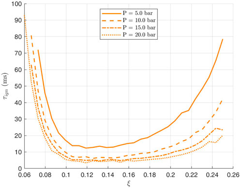
Figure 4. Variation of ammonia ignition delay with mixture fraction $\xi$ for different pressures for $T_{\text{ox}}$ = 1200 K and $T_{\text{f}}$ = 300 K.

Figure 5

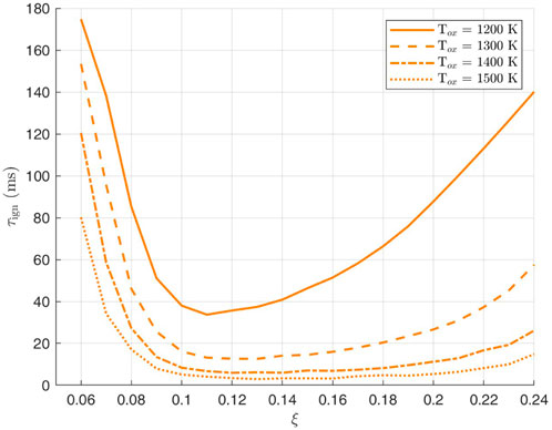
Figure 5. Variation of ammonia ignition delay with mixture fraction $\xi$ for different temperatures for $P$ = 20 bar and $T_{\text{f}}$ = 300 K.

The same procedure is followed for the decane-air mixture. In Figures 6, 7 ignition delay in terms of the mixture fraction ${\xi }_{mr}$ is presented for different pressures and temperatures. Again, similar trends are observed for lower values of $\xi$ as expected from the stoichiometric ${\xi }_{st}=0.0626$. Compared to ammonia, decane ignites quickly for high temperatures and pressures. For example, for 20 bar and $T_{ox}$ = 1200 K, the quickest ignition time for the ammonia-air system is about 35 ms, while for the decane-ar system the quickest ignition delay is about 10 ms. Overall, the higher reactivity of decane is demonstrated in the chemical scheme used. Therefore, the concept that the high reactivity fuel (decane) will autoignite before the ammonia is captured well by the current mechanism.

Figure 6

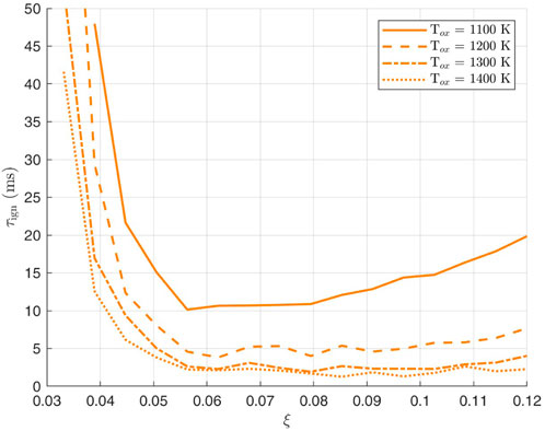
Figure 6. Variation of Decane Ignition delay with Mixture fraction $\xi$ for different temperatures for P = 20 bar.

Figure 7

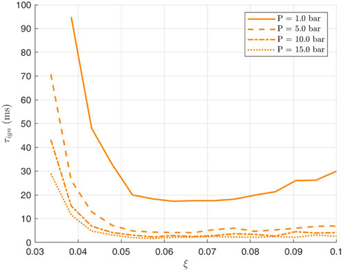
Figure 7. Variation of decane ignition delay with mixture fraction $\xi$ for different pressures for ${\text{T}}_{\text{ox}}$ = 1200 K and ${\text{T}}_{\text{f}}$ = 300 K.

3.2 Autoignition and evolution in 0D-DCMC

In this section, the 0D-DCMC exploration takes place to understand the effects of the scalar dissipation rates on the ignition of the decane-ammonia mixture. An overall description is given first, followed by a more detailed presentation of the structure of the autoignition spot and the evolution of the reaction fronts. The sensitivity to scalar dissipation rates is also shown.

3.2.1 General behaviour

The results presented in this section are from a simulation for $T_{ox}$ = 1200 K, $T_{fu}$ = 300 K and a pressure of 80 bar. The peak scalar dissipation rate is set at 10 $s^{-1}$ and a peak cross scalar dissipation rate of −5 $s^{-1}$. A three-phase evolution is usually found. The first phase is the ignition of the decane/air mixture at low values of ${\eta }_1$. The second phase consists of the diffusion of species and energy from the autoignition spot, raising the temperature in mixture fracture space and additionally transferring species to higher values of ${\eta }_1$ and ${\eta }_2$, hence igniting all mixture fractions. The third phase, if observed, corresponds to the ignition of the line ${\eta }_1=0$, which represents the ammonia/air mixing line (zero decane). A description of these three phases follows.

The evolution of the solution starts with the ignition of the decane and low ${\eta }_2$ values as seen in Figure 8. The mixture is igniting at non-zero ${\eta }_2$ values which implies that a very lean, in terms of ammonia, decane-ammonia-air mixture is more reactive than a pure decane-air mixture. The ignition ${\eta }_2$ is lower than the most reactive mixture fraction of ammonia for the given conditions, and the ignition ${\eta }_1$ is slightly richer that the decane ${\xi }_{mr}$ as quantified from the decane-air mixing layer analysis (Figure 7 for example,).

Figure 8

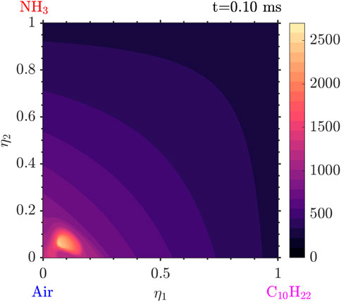
Figure 8. Temperature distribution at $t=0.1$ ms for $P=$ 80 bar, $T_{ox}$ = 1200 K, $T_{fu}$ = 300 K, $N_{\mathrm{0,1}}=N_{\mathrm{0,2}}=10$ ${\text{s}}^{-1}$, $N_{\mathit{rat}}$ = 0.5.

Following that, very quickly, the ${\eta }_2=0$ line also ignites. The scale on the right is obtained from the maximum temperature reached after having analyzed the whole simulation. The ignition fronts rapidly evolve and move to the vicinity of ${\xi }_{st}$ eventually reaching high temperatures for the whole region of mixture fractions smaller than 0.2 as seen in Figure 9. Figures 10, 11 shows the high ${\text{CH}}_2$O region migrating towards high values of ${\eta }_1$ and ${\eta }_2$ following the autoignition. Examining the same species along a single value of ${\eta }_2$ in Figure 12, we observe again the traverse as well as a single front traveling to the higher ${\eta }_1$ and a small one traveling to the low ${\eta }_1$. Furthermore, from the two-dimensional distribution the diffusion and production of ${\text{CH}}_2$O in larger ${\eta }_2$ values is evident. The presence of combustion intermediates like ${\text{CH}}_2$O in a large range of mixture fractions suggests that in pilot-ignited diesel-ammonia systems we must consider the full mixture fraction evolutions and pollutant generation and that the chemical scheme must be validated for very rich mixtures as well as lean ones.

Figure 9

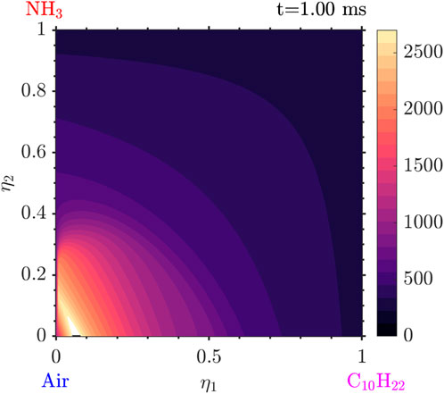
Figure 9. Temperature distribution at $t=1.0$ ms and the conditions of Figure 8.

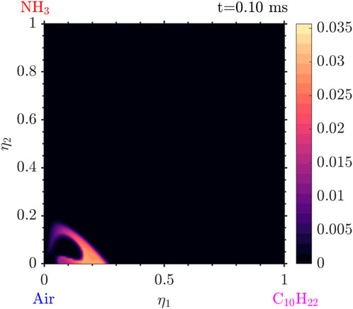
Figure 10

Figure 10. ${\mathrm{C}\mathrm{H}}_2$O mass fraction distribution at $t=0.1$ ms and the conditions of Figure 8.

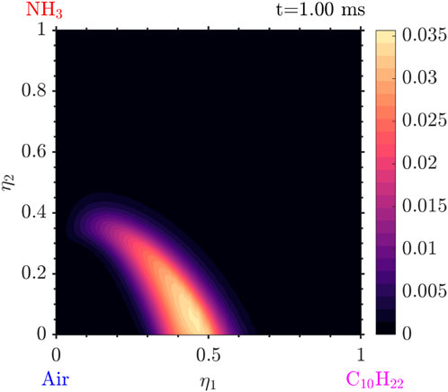
Figure 11

Figure 11. ${\mathrm{C}\mathrm{H}}_2$O mass fraction distribution at $t=1.0$ ms and the conditions of Figure 8.

Figure 12

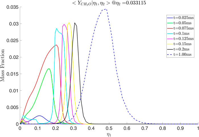
Figure 12. Conditional mass fraction of ${\text{CH}}_2$O at different instants for the conditions of Figure 8.

Tracking the temperature as well as the mass fraction for the values of ${\eta }_1$ and ${\eta }_2$ corresponding to most the reactive mixture fraction respectively in Figure 13 the rapid increase of temperature is observed reaching around 258 0K after 0.6 ms. Additionally, the pre-ignition species OH is rapidly produced and destroyed. As seen from Figure 14 that shows the distribution along the decane-air line, decane is rapidly consumed, as seen by the curvature of the green line, producing also other intermediate species such as CO and ${\text{H}}_2$ at low ${\eta }_1$. Once again, two fronts are seen for most species traveling across ${\eta }_1$. The ${\text{HO}}_2$ forms three peaks, whereas OH forms two, one around the stoichiometry of the decane and one traveling to the right, indicating two reaction fronts.

Figure 13

Figure 13. Time evolution of the temperature and the OH mass fraction at (${\eta }_1$, ${\eta }_2$) = (${\xi }_{1_{mr}}$, ${\xi }_{2_{mr}}$) and the conditions of Figure 8.

Figure 14

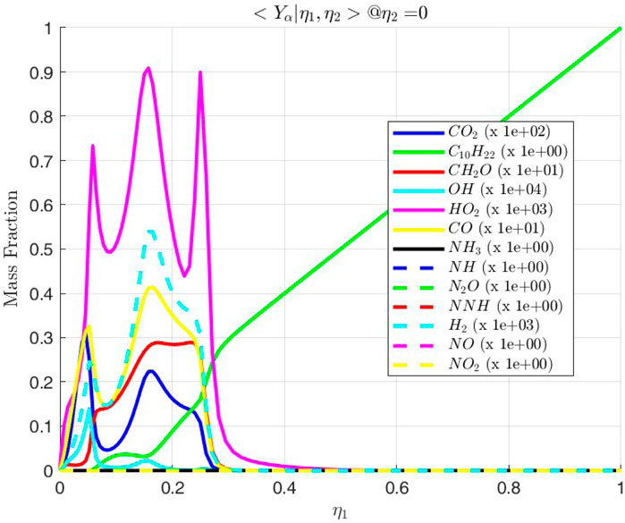
Figure 14. Conditional mass fractions of various species along the line ${\eta }_2$ = 0 and at $t=$0.1 ms. Conditions as in Figure 8.

Various species due to the presence of ammonia are also observed. In Figure 15 it is seen that the ${\text{N}}_2$O is generated around the ignition point but is eventually mainly produced in higher values of ${\eta }_2$ where the concentration of ammonia is greater (Figure 16). The initial front of ${\text{N}}_2$O has an interesting shape in the ${\eta }_1-{\eta }_2$ distribution. The front becomes significantly thicker although the peak ${\text{N}}_2$O is reduced as it moves to larger ${\eta }_2$ diffusing at the same time towards the ${\eta }_2=0$ line the same way the ${\text{CH}}_2$O is diffusing towards line ${\eta }_1=0$. The ${\text{NH}}_3$ consumption is more clear in Figure 17 where ammonia (the black line) is starting to be consumed (the curve assumes a curvature) while intermediate species such as NO and ${\text{NO}}_2$ are produced. In this figure, different species take very different shapes. The NO forms a double front while the ${\text{CH}}_2$O has one wide peak as seen before.

Figure 15

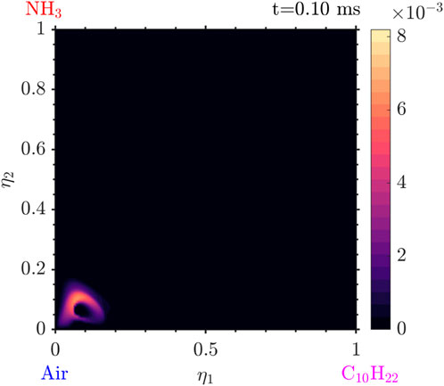
Figure 15. Mass fraction of ${\text{N}}_2\text{O}$ at $t=0.1$ ms and the conditions of Figure 8.

Figure 16

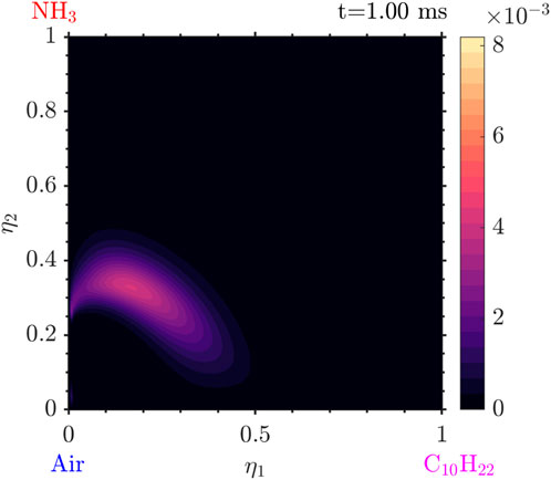
Figure 16. Mass fraction of ${\text{N}}_2\text{O}$ at $t=1.0$ ms and the conditions of Figure 8.

Figure 17

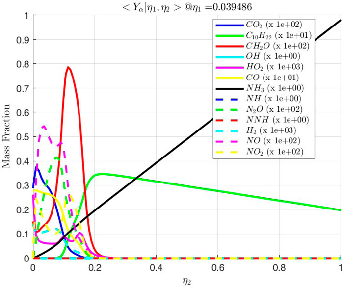
Figure 17. Conditional mass fractions as a function of ${\eta }_2$ at the indicated ${\eta }_1$ at $t=$0.1 ms and the conditions of Figure 8.

3.2.2 Intermediate phase

After autoignition, the flame grows across both mixture fractions. The diffusion flame of decane-air with no ${\text{NH}}_3$ $({\eta }_2=0)$ is eventually fully ignited and there are mixed flame structures for ${\eta }_2>0$ with progressively more presence of ${\text{NH}}_3$. Figure 18 shows the ${\eta }_2$ distributions (i.e., along the ammonia-air line) of various species at a long time after ignition and for ${\eta }_1=$0.097, i.e., slightly richer than stoichiometry for decane. The consumption of ${\text{NH}}_3$ becomes clear, while the generation of ${\text{CH}}_2$O due to the consumption of decane is also evident. Hydrogen is growing due to the decomposition of ammonia and the pyrolysis of decane. OH is peaks at the decane-air flame (i.e., somewhere at the line ${\eta }_2=0$) and is consumed at higher values of ${\eta }_2$.

Figure 18

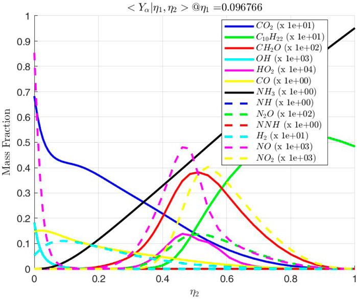
Figure 18. Conditional mass fractions vs. ${\eta }_2$ at the indicated ${\eta }_1$ at $t=$5.0 ms and the conditions of Figure 8.

3.2.3 Ignition of line ${\eta }_1=0$

The line ${\eta }_1=0$ corresponds to the air ammonia mixing line. Due to the Amplitude Mapping Model that gives $N_{{\xi }_1}$ = 0 at ${\eta }_1=0$, no species reach this line from higher mixture fractions. As a result, due to the modelling choice of the scalar dissipation model (which is the usual model in both flamelet and CMC models), this boundary follows its own characteristic time evolution. There are again pre-ignition species such as ${\text{HO}}_2$ that are rapidly produced and consumed as well as some products such as ${\text{H}}_2$ (not shown). We also see that ${\text{N}}_2$O is produced during the consumption of ammonia, which is depicted in Figure 19 where a single front forms. This front again travels to larger ${\eta }_2$ values and peaks around the stoichiometry of ammonia. The same is true for the temperature distribution in Figure 20. Initially, as seen even after 1 ms the distribution is exactly the same as the initial conditions. At some point, the line starts igniting eventually forming a front that is heading to larger ${\eta }_2$. The maximum temperature is smaller, as expected from pure ammonia, in this region. The distribution at the latest time shown in Figure 20 is similar to a conventional non-premixed autoigniting system at the moment of autoignition (Mastorakos, 2009).

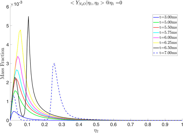
Figure 19

Figure 19. ${\mathrm{N}}_2$O along ${\eta }_2$ for ${\eta }_1=0$ at different time instants for the conditions of Figure 8.

Figure 20

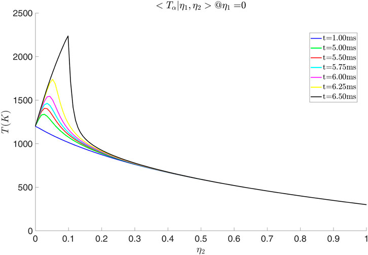
Figure 20. Temperature distribution along ${\eta }_2$ for ${\eta }_1=0$ at different time instants for the conditions of Figure 8.

3.2.4 Effects of scalar dissipation rates

Simulations with various values of scalar dissipation were performed. Examining Figures 21, 22 we observe that a positive cross-scalar dissipation rate leads to later ignition in comparison to a negative cross scalar dissipation rate. Additionally, we observe that for a higher magnitude of scalar dissipation rate the ignition is delayed in comparison to the smaller ones. Moreover, the difference in ignition time when the scalar dissipation rate is small is insignificant, as suggested by Mastorakos (2009) from analysis of autoignition in single mixture fraction. As the scalar dissipation increases, eventually autoignition does not occur, as expected (not shown here). Analyzing the evolution of the solution from Figure 23 it is evident that the diffusion of radicals is altered judging from the conditional mass fraction of ${\text{CH}}_2$O. The phenomenon again is slower for the positive cross-scalar dissipation rate. It is interesting that for high scalar dissipation rates $N_{{\xi }_1}$ and $N_{{\xi }_2}$ the diffusion of the radicals is faster to higher ${\eta }_1$ but with lower magnitude. The small scalar dissipation rate produces a thinner front with a higher concentration.

Figure 21

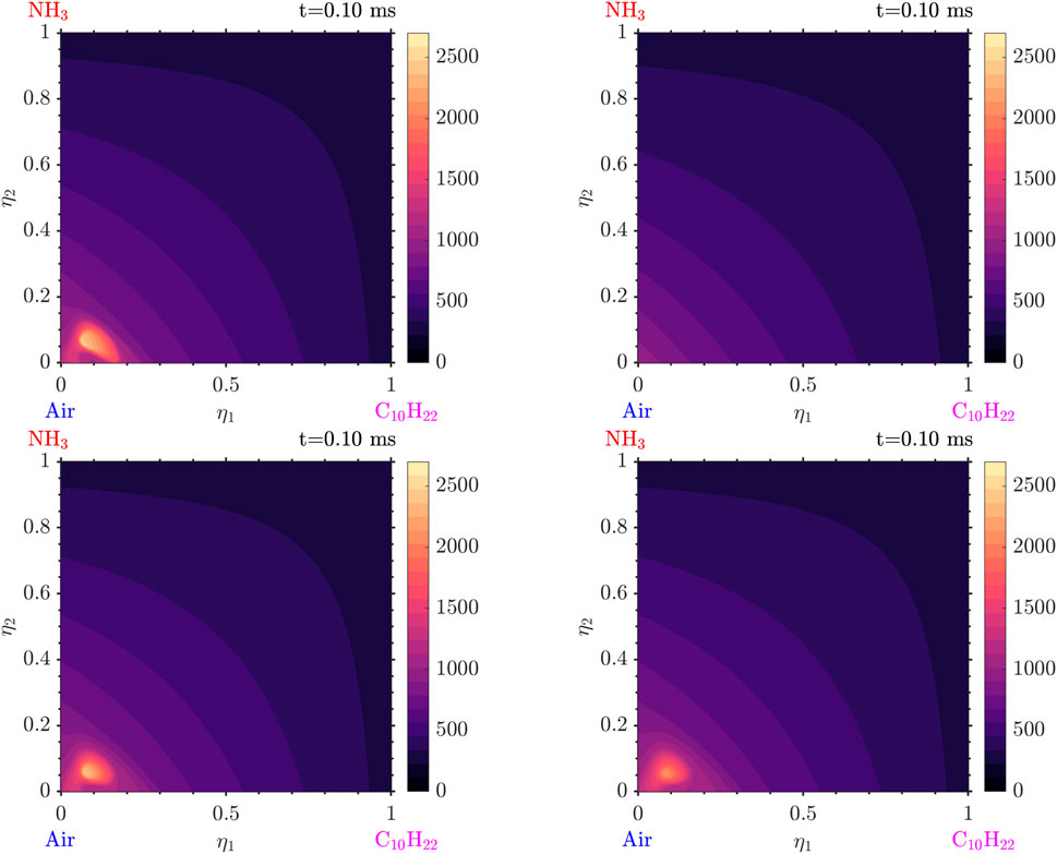
Figure 21. Distributions in ${\eta }_1-{\eta }_2$ space of the temperature at $t=$0.1 ms. From top left going clockwise: (A) ${\text{N}}_{{\xi }_1}$, ${\text{N}}_{{\xi }_2}$ = 1 ${\text{s}}^{-1}$ and ${\text{N}}_{{\xi }_1{\xi }_2}$ = −0.5 ${\text{s}}^{-1}$; (B) ${\text{N}}_{{\xi }_1}$, ${\text{N}}_{{\xi }_2}$ = 10 ${\text{s}}^{-1}$ and ${\text{N}}_{{\xi }_1{\xi }_2}$ = 5 ${\text{s}}^{-1}$; (C) ${\text{N}}_{{\xi }_1}$, ${\text{N}}_{{\xi }_2}$ = 50 ${\text{s}}^{-1}$ and ${\text{N}}_{{\xi }_1{\xi }_2}$ = −25 ${\text{s}}^{-1}$; (D) ${\text{N}}_{{\xi }_1}$, ${\text{N}}_{{\xi }_2}$ = 25 ${\text{s}}^{-1}$ and ${\text{N}}_{{\xi }_1{\xi }_2}$ = −12.5 ${\text{s}}^{-1}$.

Figure 22

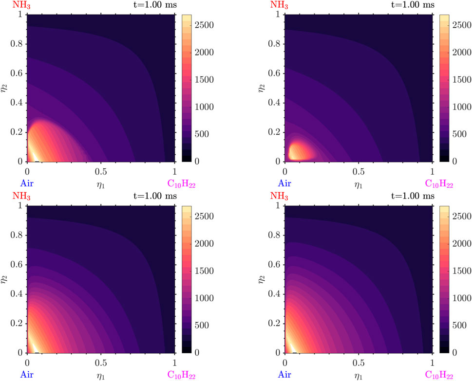
Figure 22. Distributions in ${\eta }_1-{\eta }_2$ space of the temperature at $t=$1.0 ms. From top left going clockwise: (A) ${\text{N}}_{{\xi }_1}$, ${\text{N}}_{{\xi }_2}$ = 1 ${\text{s}}^{-1}$ and ${\text{N}}_{{\xi }_1{\xi }_2}$ = −0.5 ${\text{s}}^{-1}$; (B) ${\text{N}}_{{\xi }_1}$, ${\text{N}}_{{\xi }_2}$ = 10 ${\text{s}}^{-1}$ and ${\text{N}}_{{\xi }_1{\xi }_2}$ = 5 ${\text{s}}^{-1}$; (C) ${\text{N}}_{{\xi }_1}$, ${\text{N}}_{{\xi }_2}$ = 50 ${\text{s}}^{-1}$ and ${\text{N}}_{{\xi }_1{\xi }_2}$ = −25 ${\text{s}}^{-1}$; (D) ${\text{N}}_{{\xi }_1}$, ${\text{N}}_{{\xi }_2}$ = 25 ${\text{s}}^{-1}$ and ${\text{N}}_{{\xi }_1{\xi }_2}$ = −12.5 ${\text{s}}^{-1}$.

Figure 23

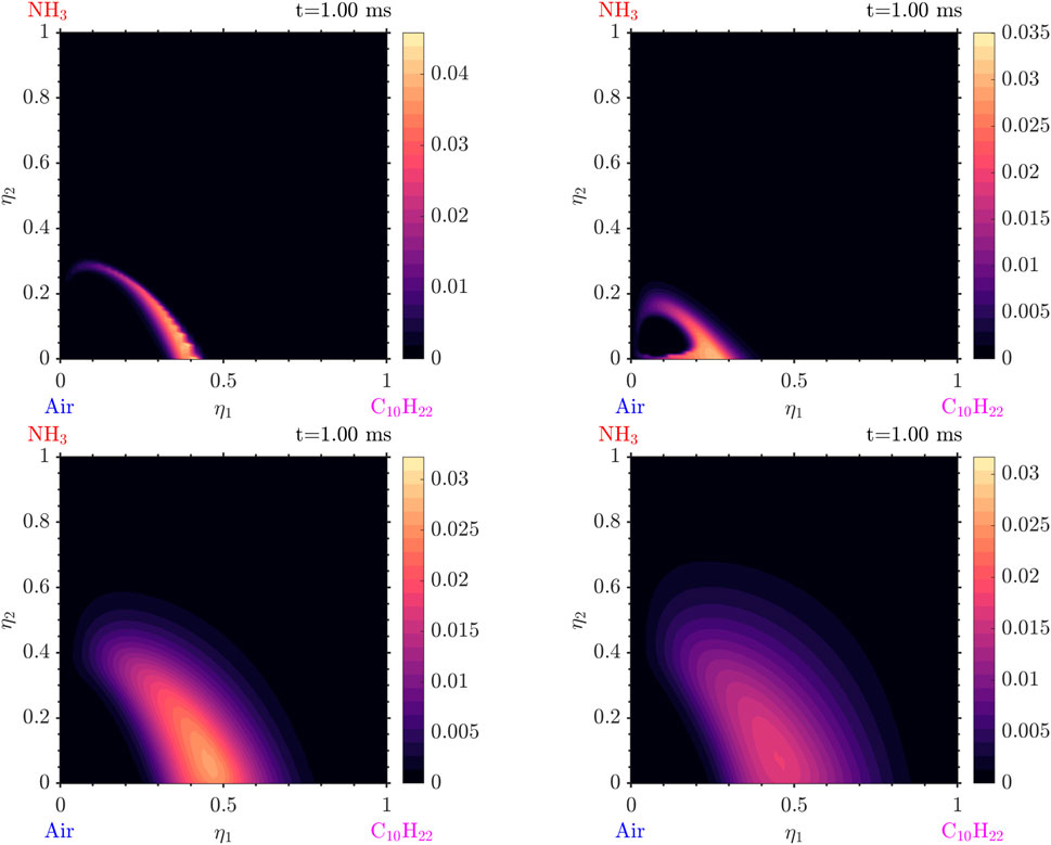
Figure 23. Distributions in ${\eta }_1-{\eta }_2$ space of the ${\text{CH}}_2$O at $t=$1.0 ms. From top left going clockwise: (A) ${\text{N}}_{{\xi }_1}$, ${\text{N}}_{{\xi }_2}$ = 1 ${\text{s}}^{-1}$ and ${\text{N}}_{{\xi }_1{\xi }_2}$ = −0.5 ${\text{s}}^{-1}$; (B) ${\text{N}}_{{\xi }_1}$, ${\text{N}}_{{\xi }_2}$ = 10 ${\text{s}}^{-1}$ and ${\text{N}}_{{\xi }_1{\xi }_2}$ = 5 ${\text{s}}^{-1}$; (C) ${\text{N}}_{{\xi }_1}$, ${\text{N}}_{{\xi }_2}$ = 50 ${\text{s}}^{-1}$ and ${\text{N}}_{{\xi }_1{\xi }_2}$ = −25 ${\text{s}}^{-1}$; (D) ${\text{N}}_{{\xi }_1}$, ${\text{N}}_{{\xi }_2}$ = 25 ${\text{s}}^{-1}$ and ${\text{N}}_{{\xi }_1{\xi }_2}$ = −12.5 ${\text{s}}^{-1}$.

Other findings include the following: as the scalar dissipation rate increases slightly smaller temperatures and slightly reduced amounts of radicals are observed. An interesting point is that, due to the different scalar dissipation rates, each mixture ignites in a different ${\eta }_1$ and ${\eta }_2$. This suggests that each fuel might be behaving differently concerning the scalar dissipation rates as each fuel has its own critical scalar dissipation rate (the scalar dissipation rate over which ignition does not take place due to the very strong mixing). As the decane is already very reactive, this leads to very high critical scalar dissipation rates for the decane-ammonia mixture. However, high values of scalar and cross-scalar dissipation rates do not allow the ammonia-air line to ignite. Also, it is observed that the production of some radicals and pollutants is changing.

In general, it is observed that high values of scalar dissipation rates can slow down reactions and therefore delay autoignition in those areas. On the contrary, the low scalar dissipation rates allow for the accumulation of species with time and temperature for the reactions to occur faster and more strongly. As a result in the general case of a flow, the mixture is expected to firstly ignite in the regions with low scalar dissipation rates and less intense mixing.

It is evident that for use in a turbulent reacting flow simulation, the magnitude of the two scalar dissipation rates, but also of the cross scalar dissipation rate, can make a large difference to the autoignition time and the evolution of species, and hence pollutants, as a function of time. Further research is needed in this area.

4 Conclusion

Simulations in a two-dimensional mixture fraction space with prescribed scalar dissipation and cross scalar dissipation rates were performed to provide insights to non-premixed autoignition of a decane-ammonia-air system. Such situations may be expected in novel ammonia engines with direct injection of both fuels and the present results offer some basic understanding of the underlying canonical problems. Due to its higher reactivity, decane ignites first and then this creates reaction fronts that move across both mixture fractions to establish eventually the non-premixed flames. For low values of the scalar dissipation, its value does not affect the autoignition time significantly, however for large values autoignition is delayed. The cross-scalar dissipation (sign and magnitude) can make a large difference in the evolution of the system, as it affects the diffusion of heat and species from the autoignition spot to the remaining unburnt fluid. Positive cross scalar dissipation leads to later autoignition compared to negative values, suggesting a diffusion of radicals into the ammonia-air mixture that act as a sink, hence delaying thermal runaway.

The present results provide a first evaluation of Doubly-Conditioned Moment Closure for hydrocarbon-ammonia systems and the results suggest that care is needed with the modelling of the cross scalar dissipation rate.

Data availability statement

The raw data supporting the conclusions of this article will be made available by the authors, without undue reservation.

Author contributions

AK: Data curation, Formal Analysis, Investigation, Methodology, Writing–original draft. EM: Conceptualization, Funding acquisition, Investigation, Project administration, Resources, Supervision, Writing–review and editing.

Funding

The author(s) declare that financial support was received for the research, authorship, and/or publication of this article. This research was partly funded by the National Research Foundation (NRF), Prime Minister’s Office, Singapore, under its Campus for Research Excellence and Technological Enterprise (CREATE) programme.

Acknowledgments

We wish to thank Drs. S. Gkantonas and B. Hariskrishnan for their help with the code. This research was partly funded by the National Research Foundation (NRF), Prime Minister’s Office, Singapore, under its Campus for Research Excellence and Technological Enterprise (CREATE) programme. For the purpose of open access, the authors have applied a Creative Commons Attribution (CC BY) license to any Author Accepted Manuscript version arising from this submission.

Conflict of interest

The authors declare that the research was conducted in the absence of any commercial or financial relationships that could be construed as a potential conflict of interest.

Publisher’s note

All claims expressed in this article are solely those of the authors and do not necessarily represent those of their affiliated organizations, or those of the publisher, the editors and the reviewers. Any product that may be evaluated in this article, or claim that may be made by its manufacturer, is not guaranteed or endorsed by the publisher.

References

Alan, C. H. (1983). Odepack, a systemized collection of ode solvers. Washington, Scientific computing.

Google Scholar

Bilger, R. W. (1993). Conditional moment closure for turbulent reacting flow. Phys. Fluids A Fluid Dyn. 5 (2), 436–444. doi:10.1063/1.858867

CrossRef Full Text | Google Scholar

Chakraborty, N., Mastorakos, E., and Cant, R. S. (2007). Effects of turbulence on spark ignition in inhomogeneous mixtures: a direct numerical simulation (dns) study. Combust. Sci. Technol. 179 (1-2), 293–317. doi:10.1080/00102200600809555

CrossRef Full Text | Google Scholar

Chin, L. L., Foscoli, B., Mastorakos, E., and Evans, S. (2021). A comparison of alternative fuels for shipping in terms of lifecycle energy and cost. Energies 14 (24), 8502. doi:10.3390/en14248502

CrossRef Full Text | Google Scholar

Curran, S., Onorati, A., Payri, R., Kumar Agarwal, A., Arcoumanis, C., Bae, C., et al. (2024). The future of ship engines: renewable fuels and enabling technologies for decarbonization. Int. J. Engine Res. 25 (1), 85–110. doi:10.1177/14680874231187954

CrossRef Full Text | Google Scholar

Harikrishnan, B., Gkantonas, S., and Mastorakos, E. (2024). LES-DCMC of dual-fuel ignition problems. American Institute of Aeronautics and Astronautics.doi:10.17863/CAM.104482

CrossRef Full Text | Google Scholar

International Maritime Organization (2015). Third IMO GHG study 2014. London: International Maritime Organization.

Google Scholar

Joung, T.-H., Kang, S.-G., Lee, J.-K., and Ahn, J. (2020). The imo initial strategy for reducing greenhouse gas (ghg) emissions, and its follow-up actions towards 2050. J. Int. Marit. Saf. Environ. Aff. Shipp. 4 (1), 1–7. doi:10.1080/25725084.2019.1707938

CrossRef Full Text | Google Scholar

Klimenko, A. Y., and Bilger, R. W. (1999). Conditional moment closure for turbulent combustion. Prog. Energy Combust. Sci. 25 (6), 595–687. doi:10.1016/s0360-1285(99)00006-4

CrossRef Full Text | Google Scholar

Kronenburg, A. (2004). Double conditioning of reactive scalar transport equations in turbulent nonpremixed flames. Phys. Fluids 16 (7), 2640–2648. doi:10.1063/1.1758219

CrossRef Full Text | Google Scholar

Lin Tay, K., Yang, W., Li, J., Zhou, D., Yu, W., Zhao, F., et al. (2017). Numerical investigation on the combustion and emissions of a kerosene-diesel fueled compression ignition engine assisted by ammonia fumigation. Appl. Energy 204, 1476–1488. doi:10.1016/j.apenergy.2017.03.100

CrossRef Full Text | Google Scholar

MAN Energy Solutions (2023). Man bw two-stroke engine operating on ammonia. Available at: https://www.man-es.com/docs/default-source/marine/tools/man-b-w-two-stroke-engine-operating-on-ammonia.pdf, (Accessed August 21, 2024).

Google Scholar

Mastorakos, E. (2009). Ignition of turbulent non-premixed flames. Prog. Energy Combust. Sci. 35 (1), 57–97. doi:10.1016/j.pecs.2008.07.002

CrossRef Full Text | Google Scholar

O’Brien, E. E., and Jiang, T.-L. (1991). The conditional dissipation rate of an initially binary scalar in homogeneous turbulence. Phys. Fluids A Fluid Dyn. 3 (12), 3121–3123. doi:10.1063/1.858127

CrossRef Full Text | Google Scholar

Perini, F., Galligani, E., and Reitz, R. D. (2012). An analytical jacobian approach to sparse reaction kinetics for computationally efficient combustion modeling with large reaction mechanisms. Energy and Fuels 26 (8), 4804–4822. doi:10.1021/ef300747n

CrossRef Full Text | Google Scholar

Perry, B. A., Mueller, M. E., and Masri, A. R. (2017). A two mixture fraction flamelet model for large eddy simulation of turbulent flames with inhomogeneous inlets. Proc. Combust. Inst. 36 (2), 1767–1775. doi:10.1016/j.proci.2016.07.029

CrossRef Full Text | Google Scholar

Peters, N. (2001). Turbulent combustion. Meas. Sci. Technol. 12 (11), 2022. doi:10.1088/0957-0233/12/11/708

CrossRef Full Text | Google Scholar

Philip, S. M. (2019). Modelling of spray combustion with doubly conditional moment closure. Flow, Turbulence and Combustion. 96, 933.

Google Scholar

Philip Sitte, M., and Mastorakos, E. (2019). Large eddy simulation of a spray jet flame using doubly conditional moment closure. Combust. flame 199, 309–323. doi:10.1016/j.combustflame.2018.08.026

CrossRef Full Text | Google Scholar

Poinsot, T., and Veynante, D. (2005). Theoretical and numerical combustion. Philadeplhia: RT Edwards Inc.

Google Scholar

Ramanathan, A., Dharmalingam, B., and Thangarasu, V. (2023). Advances in clean energy. Boca Raton: CRC Press. 1. doi:10.1201/9781003055686

CrossRef Full Text | Google Scholar

Simon, B., Mason, J., Broderick, J., and Larkin, A. (2020). Shipping and the paris climate agreement: a focus on committed emissions. BMC Energy 2 (1), 5. doi:10.1186/s42500-020-00015-2

CrossRef Full Text | Google Scholar

Thorsen, L. S., Jensen, M. S. T., Pullich, M. S., Christensen, J. M., Hashemi, H., Glarborg, P., et al. (2023). High pressure oxidation of nh3/n-heptane mixtures. Combust. Flame 254, 112785. doi:10.1016/j.combustflame.2023.112785

CrossRef Full Text | Google Scholar

Tolga Kurumus, A., Bhattacharya, A., Tamadonfar, P., and Kaario, O. (2024). A skeletal mechanism for n-dodecane/ammonia combustion and an open-source reaction scheme optimization tool. Fuel 373, 132168. doi:10.1016/j.fuel.2024.132168

CrossRef Full Text | Google Scholar

United Nations (2018). Review of Maritime transport 2018, in United Nations Conference on Trade and Development (UNCTAD), Geneva, 30 December 1964.

Google Scholar

UNFCCC (2024). United Nations Framework Convention on Climate Change (UNFCCC). The paris agreement. Available at: https://en.wikipedia.org/wiki/United_Nations_Framework_Convention_on_Climate_Change (Accessed: 2024-January-23).

Google Scholar

Valera-Medina, A., Xiao, H., Owen-Jones, M., David, W. I. F., and Bowen, P. J. (2018). Ammonia for power. Prog. Energy Combust. Sci. 69, 63–102. doi:10.1016/j.pecs.2018.07.001

CrossRef Full Text | Google Scholar

Wong, A. Y. H., Selin, N. E., Eastham, S. D., Mounaïm-Rousselle, C., Zhang, Y., and Allroggen, F. (2024). Climate and air quality impact of using ammonia as an alternative shipping fuel. Environ. Res. Lett. 19, 084002. doi:10.1088/1748-9326/ad5d07

CrossRef Full Text | Google Scholar

Yu, P., and Watanabe, H. (2023). A simplified two-mixture-fraction-based flamelet modelling and its validation on a non-premixed staged combustion system. Combust. Theory Model. 27 (1), 37–56. doi:10.1080/13647830.2022.2144460

CrossRef Full Text | Google Scholar

Zhou, X., Li, T., Chen, R., Wei, Y., Wang, X., Wang, N., et al. (2024). Ammonia marine engine design for enhanced efficiency and reduced greenhouse gas emissions. Nat. Commun. 15 (1), 2110. doi:10.1038/s41467-024-46452-z

PubMed Abstract | CrossRef Full Text | Google Scholar