Machine learning technique for the identification of two-phase (oil-water) flow patterns through pipelines

This study develops a robust machine learning model based on artificial neural networks to classify six flow patterns in oil-water two-phase flow within horizontal pipelines, a key aspect for ensuring operational efficiency, integrity, and cost-effective design in the oil and gas industry. A database comprising 1,846 experimental data points was assembled from the literature, encompassing various operating conditions, including fluid properties, superficial velocities, and pipe diameters. After evaluating 104 network configurations, the optimal model was selected, achieving an overall accuracy of 95.4%, with training, validation, and testing accuracies of 97.1%, 92.8%, and 90.3%, respectively, and a cross-entropy error of 0.024. The model demonstrated rapid convergence with a training time of only 2 s, making it a reliable and computationally efficient tool for flow pattern recognition. The outcomes of this study provide significant value for improving pipeline design, optimizing flow assurance strategies, enhancing corrosion control, and supporting real-time operational decision-making in multiphase transport systems in the oil and gas industry.

1 Introduction

The oil and gas industry has increasingly prioritized the development of advanced technologies for the accurate monitoring and characterization of multiphase flows, which involve the simultaneous movement of two or more phases, such as liquid, gas, or solid. These flows may involve immiscible substances (e.g., oil and water) or different phases of the same component (e.g., steam and liquid water) transported through a pipeline (Díaz et al., 2021; Al-Naser et al., 2016). Accurate identification of flow patterns in horizontal pipes is essential across petrochemical and fluid transport operations, as it enables better system design, enhances operational efficiency, and reduces costs (Alhashem, 2020; Soot, 1970). Proper flow pattern recognition also aids in mitigating corrosion and erosion by optimizing chemical dosing strategies, ultimately extending the lifespan of pipeline infrastructure and minimizing maintenance (Al-Sarkhi et al., 2017). Furthermore, flow patterns strongly influence heat transfer, pressure drop, and phase distribution parameters critical for the safe and efficient operation of industrial processes (Osundare et al., 2020).

Flow patterns describe the spatial arrangement of immiscible phases within a conduit and are determined by variables such as superficial velocities, fluid properties, pipe geometry, and operating conditions (El and -Sebakhy, 2010). While traditional identification techniques such as high-speed imaging, wire-mesh sensors (WMS), and gamma-ray densitometry have provided valuable insights under controlled laboratory conditions (Hernández-Cely and Ruiz-Diaz, 2020; Lum et al., 2006; Wang et al., 2024; Abduvayt et al., 2004; Cai et al., 2012; Dasari et al., 2013), their practical application in real-time industrial environments remains limited. High instrumentation costs, complex calibration procedures, and the need for expert interpretation hinder scalability and automation (Figueiredo et al., 2016; Perera et al., 2017; Su et al., 2024).

In recent years, Artificial Neural Networks (ANNs) have emerged as a promising approach for multiphase flow analysis. Unlike empirical correlations and mechanistic models that require predefined physical assumptions, ANNs can learn complex, nonlinear relationships directly from data. This makes them particularly suitable for classifying flow patterns in highly dynamic and heterogeneous systems, such as oil-water mixtures in horizontal pipelines. ANNs offer multiple advantages: they are inherently scalable, require no predefined assumptions about flow regime transitions, and can be integrated into autonomous monitoring systems for continuous operation (Chimeno-Trinchet et al., 2020; Bahrami et al., 2019; Roshani et al., 2014). Their adaptability to new data enables rapid recalibration under changing conditions, a key asset in the context of real-world operations (Qin et al., 2021; Du et al., 2019).

Multiple studies have demonstrated the effectiveness of data-driven models in improving predictive accuracy in multiphase flow systems. For example, Huang et al. (2024) applied Support Vector Machine (SVM), Random Forest (RF), and an enhanced K-Nearest Neighbor model (KNN) for regime classification in small modular reactors, while Sun et al. (2025) employed a particle swarm-optimized ANN to predict core-annular oil-water flow, outperforming conventional models in terms of accuracy and generalization. Çolak (2025) reported a high-fidelity neural model for predicting waxy crude oil viscosity with a correlation coefficient of 0.9985. These works confirm the capacity of neural architectures to capture underlying physical dynamics even in complex, nonlinear environments. Despite these advances, limitations remain—especially the limited availability of large, well-labeled datasets and the interpretability of ANN models, which are often viewed as black-box systems (Shirley et al., 2012; Xu et al., 2021).

To address these issues, recent studies have explored hybrid techniques that combine ANNs with radiation-based sensing or advanced signal processing (Roshani et al., 2021; Salgado et al., 2010). Deep learning architectures, such as Transformer Neural Networks and Long Short-Term Memory (LSTM) models, have also been applied to multiphase systems, achieving improved performance in flow pattern recognition and volume fraction estimation (Ruiz-Díaz et al., 2024a; Hernández-Salazar et al., 2024). However, most of these approaches either target gas–liquid systems or rely on small or highly specific datasets, limiting their generalizability to oil-water flow conditions.

This study addresses a critical gap in the current literature related to the accurate predictive modeling of oil-water flow patterns in horizontal pipelines using machine learning. While previous studies have often relied on limited datasets or focused on specific flow regimes, this work integrates the most comprehensive and diverse experimental database reported to date for oil-water systems. A machine learning model based on ANNs was developed to classify six distinct flow patterns, providing a robust, scalable, and generalizable tool for flow pattern recognition. This approach aims to support more reliable flow assurance, pipeline design, and operational decision-making in the oil and gas industry, by addressing limitations associated with traditional empirical correlations and mechanistic models.

2 Materials and methods

2.1 Database structuring

The database used for training, validation, and testing of the ANN was compiled from experimental studies on oil–water two-phase flow in horizontal pipes, incorporating data from 11 published works and totaling 1,846 experimental points (Figure 1).

Figure 1

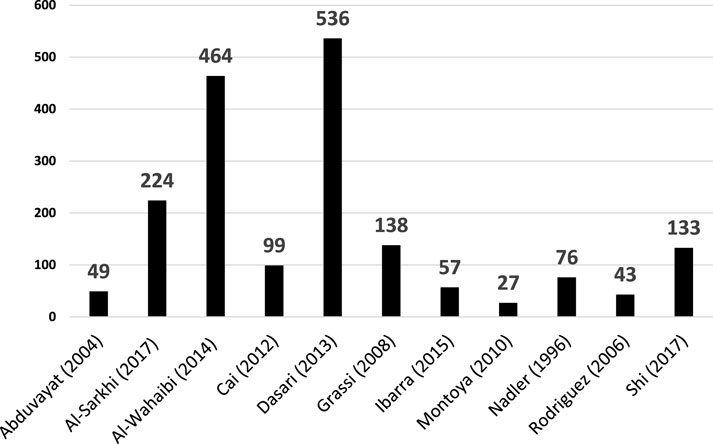
Figure 1. Distribution of data points by author.

Table 1 summarizes the main characteristics of the studies included in the database. Flow pattern data were extracted from flow regime maps reported in the selected studies. The extracted variables include superficial water velocities ($V_{sw}$) between 0.01097 and 3.7193 m/s, superficial oil velocities $(V_{so}$ between 0.01044 and 3.0392 m/s, mixture velocity $\left(V_m\right)$ between 0.02631 and 5.4714 m/s and fluid volume fractions of oil $\left(Co\right)$ and water ($\left.Cw\right)$. Other important characteristics included in the data collection to characterize the fluid are oil viscosity $\left(\mu o\right)$ between 0.00188 and 5.6 Pa $·$ s, oil density ($\left.p_O\right)$ from 800 to 910 kg/m³, and pipe internal diameter (D) between 1.9 and 10.64 cm.

Table 1

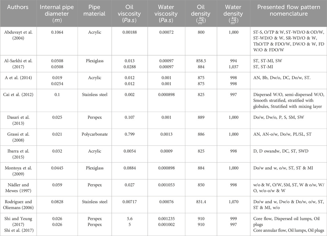
Table 1. Characteristics of the experimental database on horizontal pipelines by authors.

2.2 Liquid-liquid two-phase flow patterns in horizontal pipes

In the experimental studies reviewed, various flow patterns typically associated with oil-water two-phase flow in horizontal pipelines were identified. These include stratified flow (ST), stratified with mixture (ST & MI), slug flow (S), annular flow (AN), oil-in-water dispersion (Do/w), and water-in-oil dispersion (Dw/o). However, a notable inconsistency was observed in the terminology used across different studies to describe similar or equivalent flow regimes, which may lead to confusion in data interpretation and modeling. To address this, flow patterns exhibiting analogous physical characteristics were grouped under unified nomenclature, as shown in Figures 2, 3. The groupings are as follows:

• Annular Flow (AN): This category includes flow regimes such as Annular Flow (AN) and Annular Core Flow and Oil-in-Water Dispersion (AN-o/w).

• Oil-in-Water Dispersion (Do/w): This group comprises Dispersion of Oil in Water (Do/w), Thin Oil Layer at the Top of the Pipe and Fine Oil Dispersion in Water (ThO/TP & FDO/W), Dispersion of Oil in Water and Water (Do/w & w), Layers of Water-in-Oil and Oil-in-Water with Water (w/o–o/w, w), and Oil-in-Water Emulsion (O/W).

• Slug Flow (S): This includes Plug (P), Slug (S), Bubble (Bb), and Dispersed Oil Lumps (Oil Lumps).

• Dispersion of Water in Oil (Dw/o): This grouping includes Dispersion of Water in Oil (Dw/o), Fine Water in Oil and Fine Oil in Water Dispersions (FD W/O & FDO/W), Dispersion of Water in Oil and Water (W/O & W), and Unstable Water-in-Oil Emulsion (W/O).

• Stratified Flow (ST): This category encompasses Stratified (ST), Oil at the Top of the Pipe and Water (O/TP & W), and Wavy Stratified Flow (SW).

• Stratified Flow with Mixture (ST & MI): This includes Stratified with Mixing Layer (ST & MI), Stratified with Water Droplets in Oil and Water (SR-WD/O & W), Stratified with Water Droplets in Oil and Oil Droplets in Water (ST-WD/O & OD/W), and Dual Continuous (DC) flow patterns.

Figure 2

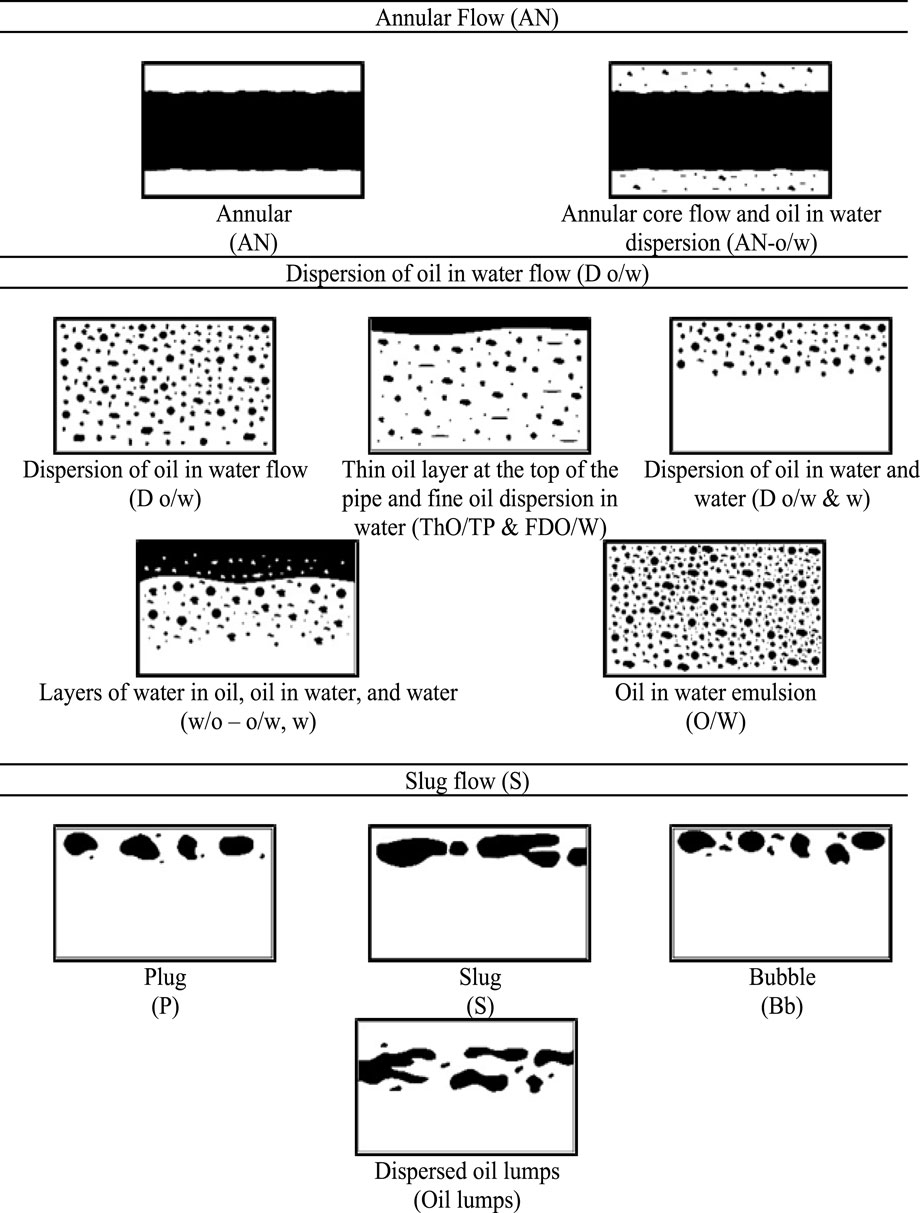
Figure 2. Grouping of flow pattern nomenclatures: annular flow, dispersion of oil in water flow, and slug flow.

Figure 3

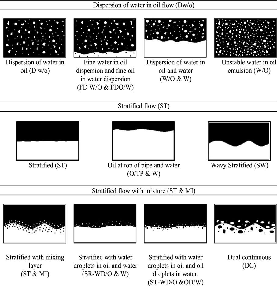
Figure 3. Grouping of flow pattern nomenclatures: dispersion of water in oil flow, stratified flow, stratified flow with mixture.

Flow pattern transitions are influenced by superficial velocities and fluid properties. For low superficial velocities of both phases, the flow pattern is stratified (ST) with complete separation of the two fluids. As the oil velocity $\left(V_{so}\right.$) increases, it begins to sweep the water, causing ripples at the interface and leading to a wavy stratified flow pattern.

Further increases in $V_{so}$, intensify the interfacial instability, causing wave break-up and dispersion of water droplets within the oil phase, resulting in the Dw/o pattern. Conversely, increasing the superficial water velocity $\left(V_{sw}\right.$) from the wavy stratified state gives rise to stratified with mixture (ST & MI), characterized by an interfacial emulsion of oil and water droplets. With continued increases in $V_{sw}$, the flow evolves into Do/w & w and eventually a uniform oil-in-water dispersion (Do/w).

At lower oil velocities, the wavy interface occasionally touches the upper wall, forming a plug or slug flow pattern with irregular, deformed plug shapes. Sometimes, this appears as larger, elongated droplets or clusters of irregular droplets.

Analysis of the compiled experimental database reveals correlations between flow pattern occurrence, pipe diameter, and fluid viscosity. In pipes with diameters equal to or greater than 0.032 m up to 0.1064 m, the flow pattern categories observed are Do/w, Dw/o, ST, and ST & MI. In contrast, smaller diameter pipes (0.019–0.032 m) also exhibit annular (AN) and slug (S) flow patterns.

Fluids with high viscosity (5 and 5.6 Pa·s) in pipes with the smallest diameters (0.026 m) only exhibited AN and S patterns. Similarly, in fluids with the next highest viscosity (0.799 Pa·s) and a pipe diameter of 0.021 m, the same flow regimes were observed. These findings suggest that high-viscosity fluids in narrower pipes are more likely to produce annular and slug flow patterns.

After the flow pattern nomenclatures were consolidated into six categories based on the nature of the observed flow, Table 2 presents the distribution of the 1,846 experimental data points compiled from the literature.

Table 2

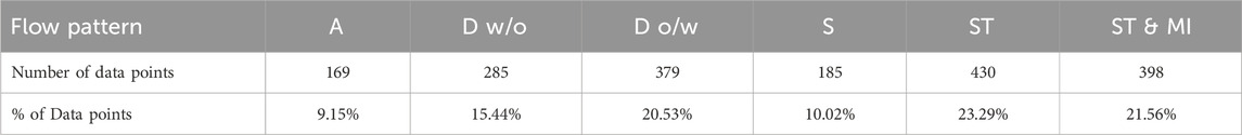
Table 2. Distribution of data points obtained according to the flow pattern.

The variables obtained from the literature to structure the database are: superficial water velocity ($V_{sw}$), superficial oil velocity ($V_{so}$), mixture velocity ($V_m$), pipe diameter (D), oil viscosity $\left(\mu o\right)$, water volumetric fraction ($C_w$), oil volumetric fraction ($C_o$) and oil density ($\left.p_O\right)$.

Superficial velocity is an important parameter when injecting fluids into a pipe, and it plays a fundamental role in forming flow patterns. The superficial velocity of a phase is the volumetric flow rate of the phase, which represents the volumetric flow rate per unit area. In other words, the superficial velocity of a phase is the velocity that would occur if that phase of the respective substance flowed through the pipe alone (Shoham, 2005). Thus, the superficial velocities of the liquid phases of water ($V_{sw}$) and oil ($V_{so}$) are respectively calculated with Equations 1, 2:

$V_{sw}=\frac{q_w}{Ap}(1)$

$V_{so}=\frac{q_o}{Ap}(2)$

where $Ap$ is the cross-sectional area of the pipe, $q_w$ is the volume flow rate of the water, and $q_o$ is the volume flow rate of the oil. The velocity of the mixture is the total volumetric flow rate of both phases per unit area, which is called the center-of-volume velocity and is given by Equation 3

$V_m=\frac{q_w+q_o}{Ap}=V_{sw}+V_{so}(3)$

The water volume fraction ($Cw$) is the fraction of a volume element in a two-phase flow field occupied by the liquid phase of water, and the oil volume fraction ($Co$) corresponding to the fraction of a volume element in a two-phase flow field occupied by the liquid phase of oil, are calculated with Equations 4, 5:

$Cw=\frac{V_{sw}}{V_{sw}+V_{so}}(4)$

$Co=\frac{V_{so}}{V_{sw}+V_{so}}(5)$

It should be remembered that the sum of the volume fraction of water and the volume fraction of oil results in 1. Adding Equations 4, 5 gives Equation 6:

$\frac{V_{sw}}{V_{sw}+V_{so}}+\frac{V_{so}}{V_{sw}+V_{so}}=1(6)$

An alternative way to calculate the volume fraction of the oil is defined in Equation 7:

$Co=1-Cw(7)$

2.3 Data pre-processing

In machine learning, complex nonlinear processes present a great diversity in the dimensionality of inputs and outputs and the size of the dataset. The complexity of neural network models and the computational load increase significantly with data dimensionality (Zhao et al., 2023). To address this problem, the dimensionality of the data should be reduced without compromising the modeling accuracy. Order reduction techniques are divided into supervised or unsupervised selection. In labeled data sets, supervised selection reveals the importance of features through correlation with the target variable and between subsets of variables (Xie et al., 2023). Supervised selection includes feature extraction and feature selection methods. Traditional extraction methods, such as partial least squares and principal component analysis (PCA), create new features in a low-dimensional space, keeping most of the relevant information, but may lack physical interpretability. Initially, we considered using this method to reduce the dimension of the database, but due to the lack of physical interpretability obtained, we chose to look for another method. On the other hand, feature selection methods choose a subset of the original features highly correlated with the system output and more interpretable, so this method was preferred. Feature selection techniques are classified into envelope, filter, and intrinsic methods. The filter method is selected, which is generally used as data preprocessing (Guyon and De, 2003), which selects variables based on statistical features, such as Pearson’s correlation, to evaluate the relationship between input variables and choose the most relevant ones (Liu et al., 2022).

2.3.1 Normalization

To train the network, it is essential to homogenize the information that will be used as input for the machine learning model. This provides the network with precise data that allows for the prediction of the relationship between the supplied variables and the pattern.

For this reason, a normalization of the input variables was performed within defined limits of 0–1. Normalization is defined as a rescaling of the original data such that it falls within a specific range (Ruiz-Díaz et al., 2024b). The input vector of the network, which contains the variables $V_{sw}$, $V_{so}$, $V_m$, $Cw$, $Co$, D, $\mu o$ and $p_O$, is normalized using Equation 8:

$X_{Normalized=\frac{X-X_{\mathit{min}}}{X_{\mathit{max}}-X_{\mathit{min}}}}(8)$

where $X_{normalized}$ corresponds to the normalized value that takes a value between 0 and 1, $X$ represents the specific value of the sample for the variable to be normalized, and $X_{\mathit{min}}$ and $X_{\mathit{max}}$ correspond to the minimum and maximum values within the dataset for the variable being normalized.

2.3.2 Statistical metrics for evaluating correlation between variables

Once the values have been normalized, the most widely used statistical evaluation method for correlation is Pearson’s correlation coefficient, which captures the linear relationship between two matrices (Xie et al., 2023). Two highly correlated variables may provide redundant information. In these cases, one of the correlated variables can be removed to simplify the process.

Equation 9 calculates Pearson’s correlation coefficient between a feature (x) and a label (y) with n training examples.

$r=\frac{{\sum }_{i=1}^n(x_i-\overline{x})\left(y_i-\overline{y}\right)}{\sqrt{{\displaystyle {\sum }_{i=1}^n}{\left(x_i-\overline{x}\right)}^2{\displaystyle {\sum }_{i=1}^n}{\left(y_i-y\right)}^2}}(9)$

where $\overline{x}$ y $\overline{y}$ are the means of the two vectors, respectively, the coefficient range is between −1 and 1, where a value of zero implies no linear correlation. Values close to 1 and −1 indicate positive and negative correlations, respectively.

Table 3 presents a correlation matrix between the input variables, showing the level of correlation between them to reduce redundancy by eliminating those with high dependence on each other.

Table 3

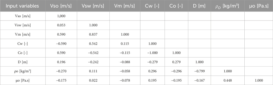
Table 3. Correlation matrix of input variables.

The qualitative interpretation of this property follows the suggestions of (Cohen, , 1988), which are widely accepted in the scientific community. Table 4 shows the classification and interpretation of the magnitude of Pearson’s correlation coefficient, applicable to any pair of variables. It considers the absolute value of the coefficient so that the magnitude is independent of the sign.

Table 4

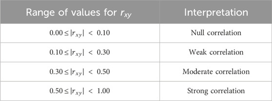
Table 4. Interpretation of the magnitude of Pearson’s correlation coefficient.

For this work, one variable from each pair of evaluated variables showing a strong Pearson correlation (with a coefficient value greater than 0.8) was removed.

The water volumetric fraction ($Cw$) and oil volumetric fraction ($Co$) showed a strong correlation with a value of −1, so the oil volumetric fraction ($Co$) was discarded from the database. Additionally, the variables superficial water velocity ($V_{sw}$) and mixture velocity ($V_m$) had a correlation coefficient of 0.837, indicating a strong correlation, and thus the mixture velocity ($V_m$) was excluded from the database.

As a result, the input variables to be used are reduced to superficial water velocity ($V_{sw}$), superficial oil velocity ($V_{so}$), water volumetric fraction ($Cw$), pipe diameter (D), oil viscosity $\left(\mu o\right)$ y and oil density ($\left.p_O\right)$.

2.3.3 Codification

The database defines the flow pattern as a categorical variable, so the label for the different categories must be coded. A number from 0 to 5 is assigned to each of the six defined flow patterns. A data preprocessing method known as one-hot encoding was used to convert the categorical variables as integers into new categorical columns with a binary value of 1 or 0. This way, each new column represents a variable category, as shown in Table 5. If this column represents a category, it is assigned a 1; otherwise, it is 0 (Liu et al., 2022).

Table 5

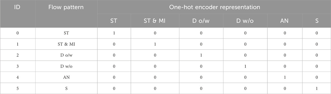
Table 5. One-Hot coding for the categorical variable.

2.4 Structuring of the artificial neural network model

This study uses an ANN to generate a model capable of predicting flow patterns. ANNs are machine learning-based tools designed for information processing and are intended to emulate how the human brain handles information (Abba et al., 2020). They are composed of different neurons as processing units connected with adjustable weights and biases. Figure 4 presents the standard structure of an artificial neuron. ANNs can be successfully applied in learning, association, classification, generalization, characterization, and optimization functions. Since ANNs can work with incomplete data and tolerate errors, they can easily create models for complex problems (Jorjani et al., 2008).

Figure 4

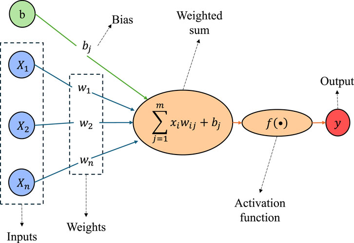
Figure 4. The standard model of an Artificial Neuron.

The ANN used in this study is a feedforward backpropagation neural network, one of the fundamental architectures in machine learning and artificial intelligence. In general, a feedforward ANN consists of multiple neural units (connected to each other by weighted connections) with activation functions, each of which takes the neuron’s net input, activates it, and produces a result that is used as input for other units (Argatov, 2019). This structure allows information to propagate from the inputs to the outputs in a single direction and uses the backpropagation algorithm to adjust the weights and minimize errors during training. This type of network structure consists of an input layer, hidden layers, an output layer, neurons, a target variable, activation functions, and a training algorithm (Abdel Azim, 2020). The presence of one or more hidden layers allows the network to model non-linear and complex functions. The mathematical expression that defines the net input $S_i$ to the neural network is obtained through Equation 10 as presented by (Hernández-Cely et al., 2022).

$S_i={\displaystyle \sum _{j=1}^m}{x}_i{w}_{ij}+b_j(10)$

where $S_i$ is the net input to node $j$ in the hidden layer, $x_i$ are the inputs to node $j$ (or outputs from the immediately preceding layer), $w_{ij}$ are the synaptic weights representing the strength of the connection between nodes $i$ and $j$, $i$ is the number of nodes, and $b_j$ is the bias associated with each node $j$.

2.4.1 Feedforward backpropagation neural network architecture

Once the information has been processed, the internal structure of the feedforward backpropagation ANN is defined. Figure 5 presents a general diagram of this type of neural network architecture. It can be seen that in the first hidden layer, the number of inputs is defined, which is a vector containing the input parameters used to generate predictions. Then, the output layer is described, producing the final prediction of the model. The number of neurons in this layer corresponds to one neuron per class in multi-class classification problems. In this case, there are six neurons, one for each flow pattern developed inside the horizontal pipes. The selection of the specific topology of the ANN is explained in Section 2.5.

Figure 5

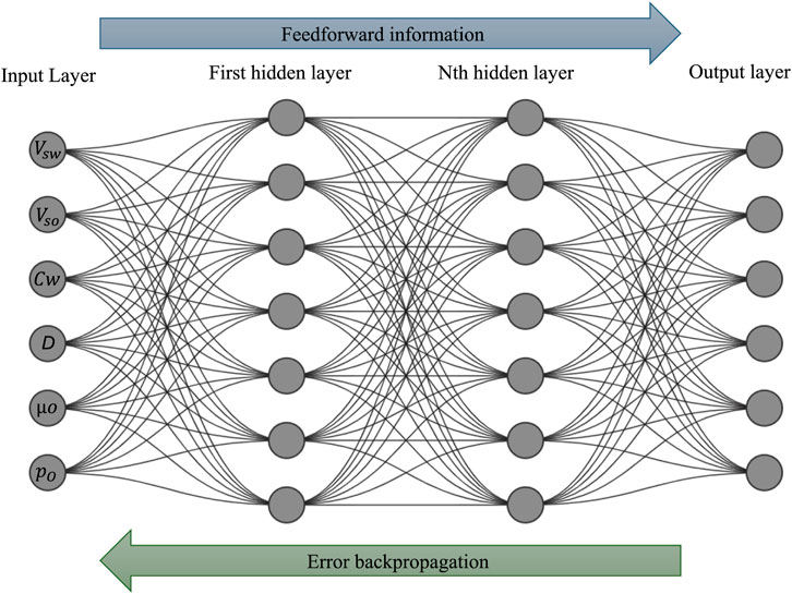
Figure 5. The general structure of a Feedforward Backpropagation ANN.

2.4.2 Activation functions

The neurons in the hidden layer use the sum of the inputs with synaptic weights as a propagation rule to apply an activation function, which introduces non-linearity to the ANN, allowing the model to learn and represent complex data relationships (Goodfellow et al., 2016). Commonly used activation functions for function approximation are the sigmoid, hyperbolic tangent, and linear functions, with the sigmoid being the most widely used for non-linear relationships. The sigmoid activation function was selected for the hidden layers based on its well-documented effectiveness in multi-class classification tasks involving moderate-sized datasets. This function provides smooth, bounded outputs in the [0, 1] range, which complements the Softmax function used in the output layer. To validate this choice, preliminary tests were conducted using activation functions such as ReLU and hyperbolic tangent (tanh). While ReLU is computationally efficient and widely adopted in deep learning, it introduced instability during training in our model, particularly in configurations with multiple hidden layers. The tanh function also yielded lower validation accuracy and slower convergence compared to sigmoid. Therefore, the sigmoid function was retained for its superior consistency and overall model performance in this specific classification task. This study uses the sigmoid activation function in the hidden layers. This function converts any real value into a value between 0 and 1, making it helpful in predicting a binary class label. In the output layer, the Softmax activation function is used. Softmax is typically employed as the final activation function in a neural network to transform outputs into a probability representation, bounding the values in a range from 0 to 1 in a vector, such that the sum of all probabilities in the vector equals 1 for all possible outcomes or classes. Mathematically, the sigmoid activation function, according to (Razavi et al., 2003), is defined as in Equation 11:

$f\left(y_j\right)=\frac{1}{1+e^{-y_j}}(11)$

where $y_j$ is the output of node $j$ and, in turn, serves as the input element to the nodes of the next layer.

The Softmax activation function $S$ defined by Equation 12 as:

${S\left(y\right)}_i=\frac{\exp \left(y_i\right)}{{\displaystyle {\sum }_{j=1}^n}\exp \left(y_j\right)}(12)$

where $y$ is an input vector to a Softmax function, $y_i$ is the i-th element of the input vector, which can take any value between negative and positive infinity, $\mathit{exp}\left(y_i\right)$ is the standard exponential function applied to $y_i$. The term ${\displaystyle \sum _{\mathrm{j}=1}^{\mathrm{n}}}\exp \left({\mathrm{y}}_{\mathrm{j}}\right)$ refers to a normalization term. This ensures that the output vector values sum to 1 for the i-th class, and each value is within the range of 0–1, thereby forming a valid probability distribution.

2.4.3 Loss function

It is worth mentioning that machine learning models learn through a loss function, which is a method for determining how effectively a specific algorithm models the provided data. The loss function will generate a high value if the predictions are far from the actual results. For the problem at hand, the chosen loss function, an important parameter indicating the performance of the ANN model, is cross-entropy loss, as it is the most common for multi-class classification problems.

This cross-entropy loss increases as the probability obtained from the Softmax function diverges from the true label. Cross-entropy loss is measured as a number between 0 and 1, where 0 represents a perfect model. Mathematically, it is defined as shown in Equation 13:

$L_{CE}=-\frac{1}{n}{\displaystyle \sum _{i=1}^n}{\displaystyle \sum _{j=1}^c}{T_j}^{\left(i\right)}\log \left({S_j}^{\left(i\right)}\right)(13)$

where $c$ represents the classes, $n$ is the number of samples, $T_j$ is the true label, and $S_j$ is the Softmax probability for the jth class.

A training algorithm must be implemented for the neural network to learn the relationship between the data, and a training algorithm must be implemented. Gradually, during the training of the model, the synaptic weights are adjusted iteratively to minimize prediction error. Adjusting the synaptic weights defines the model’s training (Gómez et al., 2004), and as the model continues to train and the loss function error is minimized, the model is said to be learning.

2.5 Model selection and evaluation

2.5.1 Artificial neural network topology

At this stage of designing the ANN, the network topology is defined, which involves the structural configuration of the model, including the number of layers, the number of neurons per layer, and the training algorithm. This stage is critical because the topology directly influences the model’s representation capacity and learning effectiveness. The topology must be tailored to the specific problem being addressed. Due to the lack of standardized techniques for this task, an approach based on experience and trial-and-error is often used, testing various configurations until finding the most suitable one for the flow pattern classification problem (Chauvin and Rumelhart, 1995).

2.5.2 Optimization parameters

An iterative and systematic experimental process uses MATLAB’s Neural Network Pattern Recognition tool to select the ANN topology. Various ANN configurations are created and optimized within the tool. Choosing an appropriate training algorithm is crucial to optimize the adjustment of synaptic weights and minimize the loss function value. Therefore, the five most commonly used and recommended training functions for classification problems in MATLAB are evaluated: TRAINSCG (Scaled Conjugate Gradient), TRAINBFG (BFGS Quasi-Newton), TRAINRP (Resilient Backpropagation), TRAINCGP (Polak-Ribiére Conjugate Gradient), and TRAINCGB (Conjugate Gradient with Powell/Beale Restarts). Additionally, key characteristics are considered in the model selection process to evaluate its performance, such as accuracy, loss function value, and ANN training time. Accuracy is obtained from the data in the confusion matrix, the loss function value is determined according to Equation 13, and training time is measured in seconds, indicating how long the ANN takes to train.

2.5.3 Confusion matrix

The confusion matrix is a fundamental tool in machine learning for evaluating the performance of a classification model. It allows for the visualization of the model’s predictions against actual values and facilitates the identification of specific errors (Powers, 2011). It is necessary to calculate its components, such as True Positives (TP), False Negatives (FN), False Positives (FP), and True Negatives (TN). Several essential metrics can be derived from the confusion matrix to assess the model’s performance, including precision, recall, F1 score, and accuracy. Precision is the proportion of true positives over the total predicted positives, recall is the proportion of true positives over the total actual positives, the F1 score is the harmonic mean of recall and precision, and accuracy is the proportion of all correct predictions. These are respectively defined by Equations 14–17

$Precision=\frac{TP}{TP+FP}(14)$

$Recall=\frac{TP}{TP+FN}(15)$

$F1=2*\frac{Precision*Recall}{Precision+Recall}(16)$

$Accuracy=\frac{TP+TN}{TP+TN+FP+FN}(17)$

3 Results

This section presents the numerical values obtained from the iterative and organized process of testing and selecting the ANN structure. These results were derived from all the simulations carried out under different topological configurations, in which all the data from the simulation process were recorded. Subsequently, an analysis and model selection were performed to identify the one that presented the best performance results in predicting flow patterns. Various configurations were structured by adjusting parameters such as the training algorithm, the number of hidden layers, and the number of neurons in each hidden layer.

For each of the structured models, the following parameters were kept constant: the data distribution was set at 70% for the training stage, 15% for the validation stage, and 15% for the testing stage. The activation function for all hidden layers was the sigmoid function, and the Softmax activation function was used for the output layer. The error function to be optimized was cross-entropy, and two retrainings were performed for each configuration. Modifying the script lines generated by MATLAB’s Neural Network Pattern Recognition tool made all adjustments to the parameters. All experimental tests were conducted on an MSI Raider GE76 computer with a 12th Gen Intel(R) Core (TM) i7-12700H 2.70 GHz processor, 16 GB of installed RAM, and a 64-bit operating system, X64 processor.

Table 6 presents the configurations generated with different combinations of parameters to be applied to the ANN models. They were evaluated according to the training functions shown in Table 7. In this manner, 200 ANN tests were initially performed based on 100 different parameter configurations, from which the models that yielded the best performance values were identified, focusing on cross-entropy and those achieving over 90% accuracy in flow pattern predictions. Once these configurations were identified, the ANN model tests were repeated to obtain a second verification of the results and to filter the evaluated topologies to those that demonstrated the highest prediction accuracy across both retraining for flow patterns.

Table 6

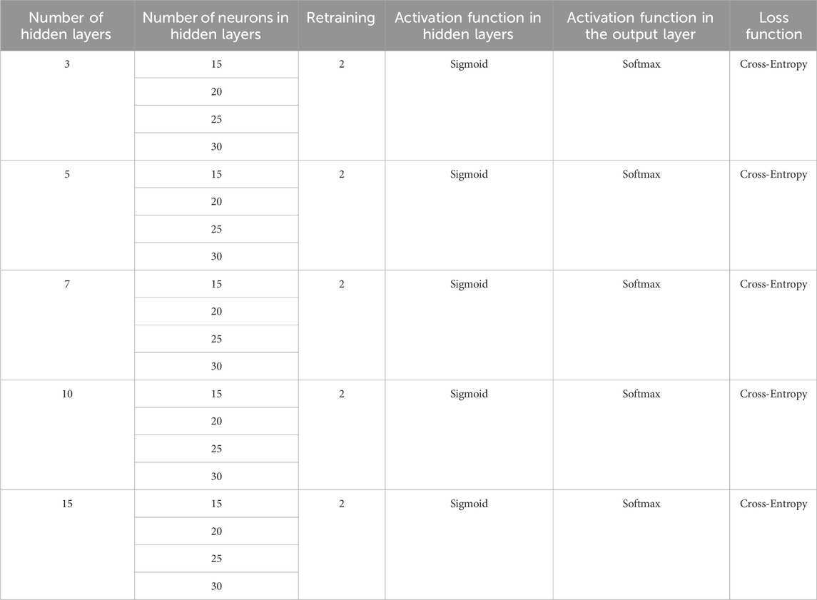
Table 6. Parameter configurations for different structured ANNs.

Table 7

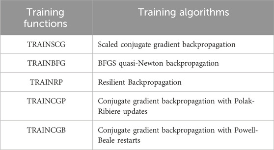
Table 7. Training algorithms to be evaluated.

Table 8 presents the best results obtained from testing the different configurations in the topology for each training function. Additionally, it.

Table 8

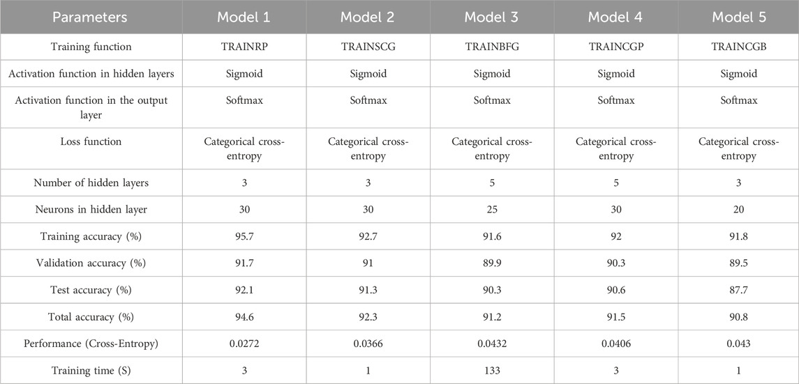
Table 8. Accuracy and performance results in models obtained under different parameter configurations.

Table 8 presents a comparative summary of five ANN models trained with different algorithms, showing the accuracy values from the confusion matrices for the training, validation, and testing stages, as well as from the overall confusion matrix. All models use the same activation and loss functions but vary in topology and training method. Model 1 (TRAINRP) achieved the best overall performance, with the highest total accuracy (94.6%), strong validation and test accuracy, and a short training time (3 s), making it the most balanced and efficient configuration. Model 2 (TRAINSCG) also performed well, offering good accuracy (92.3%) with the shortest training time (1 s), indicating its suitability for fast iterative training. Model 3 (TRAINBFG) achieved competitive accuracy (91.2%) and low cross-entropy loss, but required 133 s to train. This extended time is due to the computational complexity of the BFGS algorithm and the use of a deeper network (5 hidden layers). Models 4 and 5 (TRAINCGP and TRAINCGB) yielded acceptable but slightly lower accuracies and higher loss values, despite fast training times. Overall, the results highlight TRAINRP as the most effective training function in terms of performance and computational efficiency. Once the learning algorithm was defined, a final experiment was conducted, maintaining the established parameters from Model 1, except for the number of neurons per hidden layer. This was further evaluated with 40, 50, 60, and 70 neurons to observe the performance and accuracy of the ANN model.

Table 9 presents the results of training the ANN model with 40, 50, 60, and 70 neurons in the hidden layers. The minimum cross-entropy error values were identified from the information collected, being 0.0342 and 0.024 for 40 and 50 neurons in the hidden layers, respectively, and total accuracy values of 92.7% and 95.4%. By analyzing the information presented in Table 9, it was determined that the optimal ANN for developing the predictive flow pattern model for two-phase (oil-water) flow in a horizontal pipe is the one that integrates the Resilient Backpropagation learning algorithm with three hidden layers, each with 50 neurons. The configuration of the selected model’s parameters is presented in Table 10.

Table 9

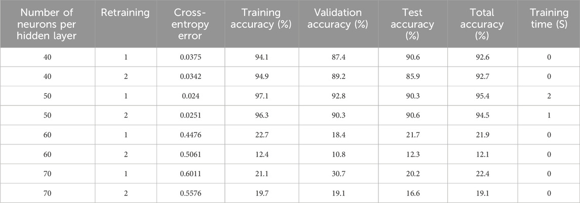
Table 9. Results of varying the number of neurons per hidden layer using the Resilient Backpropagation learning algorithm in ANN model 1.

Table 10

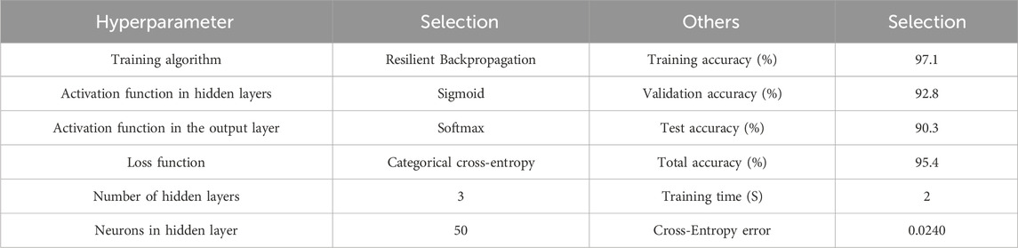
Table 10. Configuration of parameters and results of the selected ANN Model.

With the selected ANN configuration, the model achieved a cross-entropy loss of 0.024, with a training accuracy of 97.1%, validation accuracy of 92.8%, and test accuracy of 90.3%. The overall classification accuracy, calculated from the complete confusion matrix across all data partitions, reached 95.4%, making this configuration the most effective among the 104 models evaluated. Figure 6 illustrates the evolution of cross-entropy loss throughout the training process for the training, validation, and testing stages. The best validation performance was observed at epoch 103, with a cross-entropy value of 0.03213. The training process was terminated at epoch 109 using early stopping criteria, which halts training when the validation error does not improve over six consecutive epochs (patience = 6). The final model thus corresponds to the point of minimum validation error, ensuring both high accuracy and generalization.

Figure 6

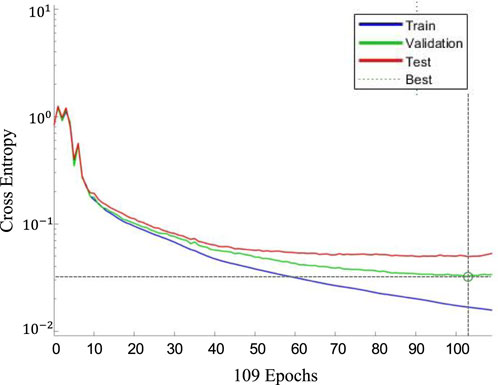
Figure 6. Variation of cross-entropy due to iteration change in the ANN with the selected configuration.

The model’s performance and accuracy data are complemented by an error histogram, presented in Figure 7, showing the error values obtained in each stage of the ANN’s development. The histogram exhibits a centered normal distribution, with a clear central and narrow tendency towards error values close to zero, indicating that the model is well-trained and highly accurate. The high frequency observed in the central column, where most data comes from the training, validation, and testing stages, suggests that the model generalizes well and does not overfit the training data.

Figure 7

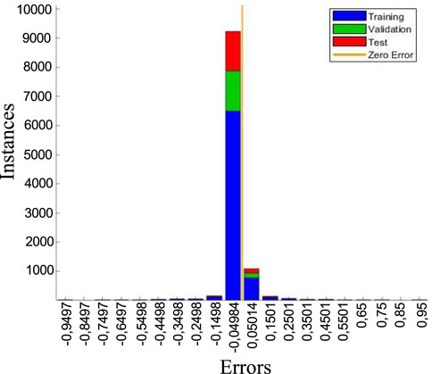
Figure 7. Error histogram in the training, validation, and testing stages for the ANN model.

Figure 8 illustrates the ROC (Receiver Operating Characteristic) curves corresponding to the (a) training, (b) validation, (c) testing, and (d) overall stages of the ANN model. These plots provide a visual assessment of the classifier’s ability to distinguish between the six flow pattern classes across different stages of model development.

Figure 8

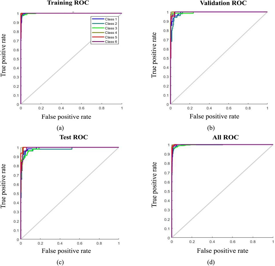
Figure 8. ROC curve in (a) training stage, (b) validation stage, (c) testing stage, (d) overall confusion matrix.

In each subplot, the ROC curve compares the model’s true positive rate (TPR) against the false positive rate (FPR) across various classification thresholds. The area under each ROC curve (AUC) serves as a scalar metric for the model’s discriminative power, with values closer to 1 indicating near-perfect classification. The diagonal line in each plot represents the performance of a random classifier (AUC = 0.5), which serves as a baseline for comparison.

In the training stage (Figure 8a), the ROC curves demonstrate excellent separation between classes, with all curves approaching the top-left corner, reflecting high sensitivity and low false positive rates. This indicates that the model has learned the patterns in the training data effectively. A similar trend is observed during the validation stage (Figure 8b), suggesting that the model maintains generalization capability and avoids overfitting. The testing stage (Figure 8c) also shows strong ROC curves, further validating the model’s robustness and confirming that the classification performance remains stable on previously unseen data.

The overall ROC plot (Figure 8d), which aggregates performance across all stages, shows that the classifier consistently performs well across the six flow pattern categories. The concentration of the curves toward the upper-left corner signifies high true positive rates with minimal false classifications. These results reinforce the ANN model’s capacity to reliably differentiate among complex flow regimes under varying operating conditions.

Together, these ROC analyses underscore the high sensitivity and specificity of the selected ANN configuration. The network’s performance across all evaluation stages aligns with the confusion matrix results and statistical metrics, providing strong evidence of the model’s effectiveness for real-time multiphase flow pattern recognition in horizontal oil-water pipeline systems.

Figure 9 presents the confusion matrices obtained during the (a) training, (b) validation, (c) testing, and (d) overall evaluation phases for the selected ANN model. These matrices provide a detailed breakdown of the model’s prediction performance for each of the six flow pattern categories: stratified, stratified with mixture, oil-in-water dispersion, water-in-oil dispersion, annular, and slug.

Figure 9

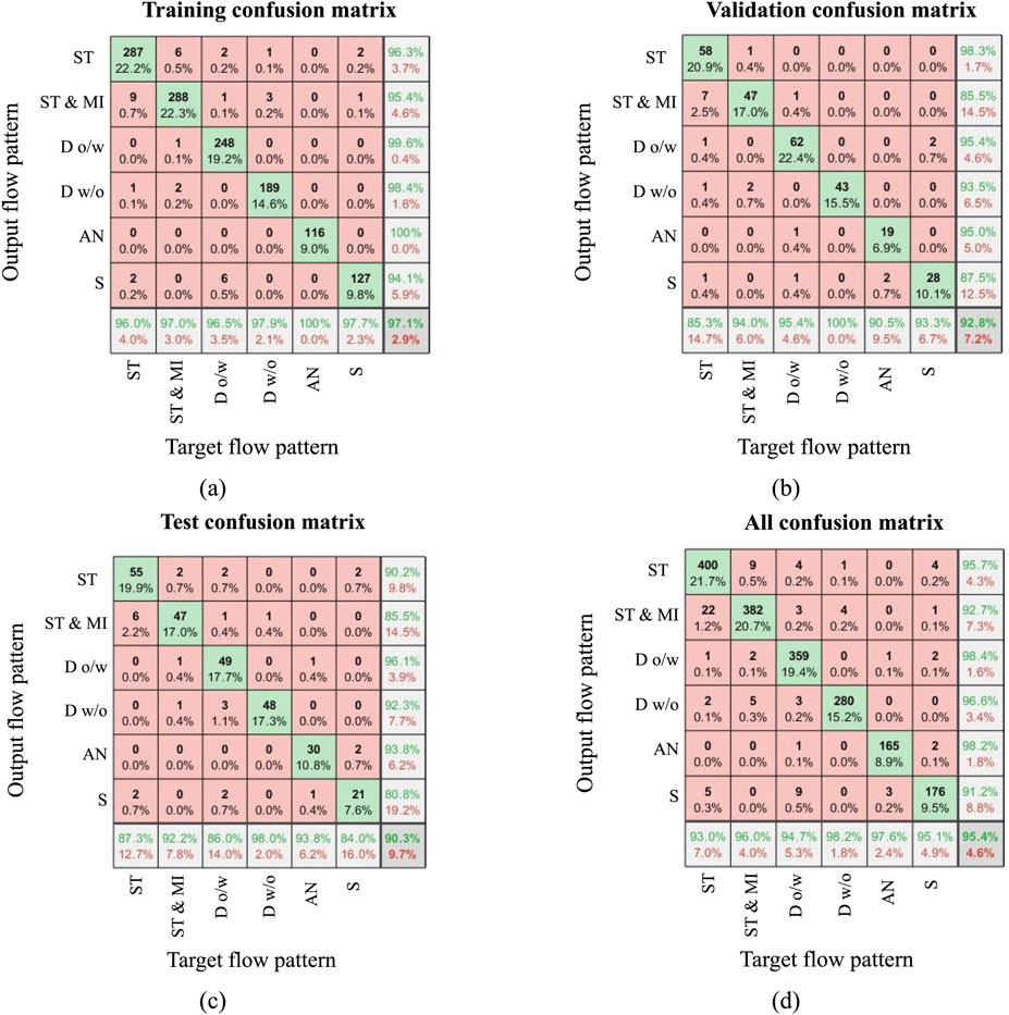
Figure 9. Confusion matrix in (a) Training stage, (b) Validation stage, (c) Testing stage, (d) Overall confusion matrix. The reported accuracy values represent overall classification accuracy, not class-averaged metrics.

In each matrix, the diagonal elements represent the TP—that is, the number of instances correctly classified as a specific flow pattern. Off-diagonal entries reflect misclassifications, further categorized as FP and FN. A false positive occurs when the model incorrectly predicts a sample as belonging to a given class, while a false negative arises when the model fails to recognize an instance of that class. The TN, although not explicitly visible in the matrix, can be inferred as all other correctly classified instances not associated with the current class under evaluation.

The confusion matrices show a high concentration of values along the diagonal, indicating that the majority of predictions across all evaluation stages were correct. In the training stage (Figure 9a), the model achieved an accuracy of 97.1%, confirming its strong capacity to learn from the dataset. During the validation phase (Figure 9b), accuracy slightly decreased to 92.8%, suggesting that the model generalizes well to unseen data while maintaining high predictive consistency. The testing stage (Figure 9c) resulted in an accuracy of 90.3%, demonstrating reliable performance even on completely new data. Finally, the overall confusion matrix (Figure 9d), which aggregates predictions from all stages, reports a high total classification accuracy of 95.4%, underscoring the robustness and generalization capability of the selected ANN configuration.

Beyond overall accuracy, the confusion matrices also reveal class-specific performance trends. Certain patterns such as Do/w and Dw/o exhibit nearly perfect classification with minimal off-diagonal values, suggesting that the model captures their distinguishing features with high fidelity. Meanwhile, flow patterns such as S and ST & MI, which are often characterized by overlapping or transitional behaviors, show slightly higher misclassification rates, pointing to the physical complexity and subtlety involved in accurately separating these regimes.

In Table 11, the respective precision, recall, and F1 values for each flow pattern are presented, along with the accuracy values for both the confusion matrix in the testing stage and the overall confusion matrix, calculated according to Equations 14–17. Accuracy refers to the proportion of all correctly classified samples across all classes, calculated as (sum of diagonal entries)/(total number of samples). Precision, recall, and F1-score are computed per class, and their values reflect the model’s behavior in distinguishing each individual flow pattern. The averages refer to the mean of these class-specific values. For example, for the testing stage, referencing the ST pattern, the true positives value is TP = 55, from the diagonal entry corresponding to the ST class in the test stage confusion matrix, see Figure 9c. By summing the other values on the main diagonal, the TN total is 195. Summing the other values in the ST row gives the FP as 6, and summing the other values in the ST column gives the FN as 8. Notice that for a multiclass confusion matrix, accuracy is computed as the sum of all correct predictions (250) over the total number of predictions (277). The values shown for precision, recall, and F1 are class-specific, but accuracy is aggregate.

Table 11

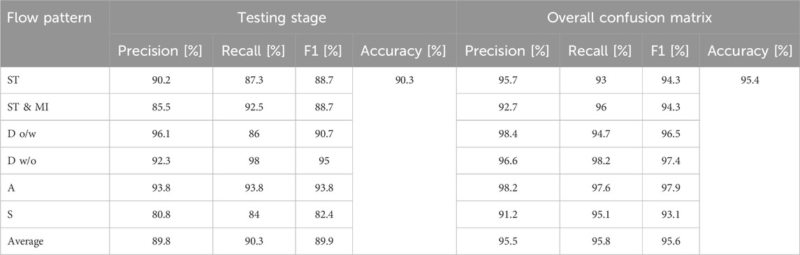
Table 11. Metrics to evaluate model performance across different flow patterns based on the confusion matrix.

Based on the information shown in Table 11, the following average values were determined for the different flow patterns within the testing stage of the model: an average precision of 89.8%, an average recall of 90.3%, an average F1 score of 89.9%, and an accuracy of 90.3%. From the overall confusion matrix, an average precision of 95.5%, an average recall of 95.8%, an average F1 score of 95.6%, and an accuracy of 95.4% were obtained.

To ensure the credibility of the proposed ANN model, the dataset was randomly partitioned into 70% for training, 15% for validation, and 15% for testing. The model’s performance was evaluated through multiple statistical metrics, including accuracy, precision, recall, F1-score, and cross-entropy error, across all three data partitions. Confusion matrices and ROC curves were used to provide a comprehensive visualization of the classifier’s behavior. Additionally, retraining was conducted for each configuration to verify repeatability and robustness, with consistent outcomes observed between runs.

The credibility of the model is reinforced by the use of a large and diverse dataset compiled from 11 independent experimental studies, representing a wide range of fluid properties, pipe diameters, and flow regimes. This diversity enhances the model’s generalization capabilities and supports its applicability across varied operating conditions.

4 Conclusion

A two-phase oil-water flow database in horizontal pipes was structured based on information reported in the literature by various authors, yielding 1,846 experimental data points. The dataset included parameters related to oil-water multiphase flows, such as the superficial velocities of the oil and water fluids, water volumetric fraction, pipe diameter, oil viscosity, and oil density. Six representative flow pattern categories were defined and standardized: stratified, stratified with mixture, slug, annular, oil-in-water dispersion, and water-in-oil dispersion.

An ANN model using feedforward backpropagation was developed in MATLAB^® and its Neural Network Pattern Recognition tool. Through an iterative and systematic experimental process, 339 training sessions were performed based on 104 different ANN topological configurations to select the optimal model. The final model consisted of an input layer with six neurons corresponding to each input variable, three hidden layers with 50 neurons each, and an output layer with six neurons. The resilient backpropagation training algorithm was employed, with sigmoid activation functions in the hidden layers and softmax in the output layer, using cross-entropy as the loss function.

The developed ANN model demonstrated outstanding performance, achieving a training accuracy of 97.1%, a validation accuracy of 92.8%, a testing accuracy of 90.3%, and an overall accuracy of 95.4%. These results suggest that the trained model is highly effective at predicting the six flow patterns. Notably, the training process required only 2 s, indicating high computational efficiency. The precision of the ANN model in recognizing flow patterns suggests opportunities to optimize pipeline design and maintenance processes by estimating critical process parameters, such as pressure gradients and volumetric fractions in the flow system.

Beyond its strong predictive performance, the proposed model demonstrates substantial potential for practical deployment in industrial settings. Its ability to classify flow patterns with high reliability and low latency makes it suitable for integration into real-time monitoring systems, such as SCADA platforms or embedded diagnostic tools for pipeline infrastructure. This opens opportunities for automated decision-making in flow assurance, chemical dosing optimization, corrosion control, and maintenance scheduling, all of which are critical for operational safety and efficiency in the oil and gas industry.

Additionally, because the model was trained on a diverse and comprehensive experimental database, it offers high scalability and adaptability across a broad range of pipeline geometries, fluid properties, and operating conditions. These features enable its use in varied field applications, including offshore platforms, onshore transport systems, and laboratory-scale experimental setups, without significant retraining or hardware constraints.

Nevertheless, several limitations should be acknowledged. First, the model was trained on laboratory-generated data, which may not fully capture the complexities encountered in field-scale operations, such as temperature fluctuations, scale deposition, or transient behaviors. Second, an imbalance in the number of data points per flow pattern category may lead to classification bias toward the majority classes. Third, as with most neural network architectures, the model functions as a “black box”, offering limited interpretability regarding the physical mechanisms underlying its predictions.

To address these limitations, future work will focus on external validation using new experimental data from controlled laboratory test rigs and real pipeline operations. The integration of explainable AI techniques and comparisons with alternative machine learning models will also be explored to enhance interpretability and benchmarking. Moreover, the construction of a more balanced and expanded database, particularly in underrepresented flow pattern classes, is recommended to enhance robustness and reduce bias in predictive performance.

Data availability statement

The original contributions presented in the study are included in the article/supplementary material, further inquiries can be directed to the corresponding author.

Author contributions

DU-T: Conceptualization, Formal Analysis, Investigation, Writing – original draft. CR-D: Conceptualization, Data curation, Methodology, Validation, Writing – review and editing. OG-E: Conceptualization, Formal Analysis, Funding acquisition, Investigation, Methodology, Project administration, Supervision, Validation, Writing – review and editing.

Funding

The author(s) declare that financial support was received for the research and/or publication of this article. This work was supported by Universidad Industrial de Santander (grant number VIE-3714, VIE-3716, VIE-3913).

Acknowledgments

Carlos Ruiz gratefully acknowledges the support of the Ministerio de Ciencia, Tecnología e Innovación of Colombia. We acknowledge the support of the Industrial Multiphase Flow Laboratory (LEMI) of the Sao Carlos School of Engineering, University of São Paulo.

Conflict of interest

The authors declare that the research was conducted in the absence of any commercial or financial relationships that could be construed as a potential conflict of interest.

Generative AI statement

The author(s) declare that no Generative AI was used in the creation of this manuscript.

Publisher’s note

All claims expressed in this article are solely those of the authors and do not necessarily represent those of their affiliated organizations, or those of the publisher, the editors and the reviewers. Any product that may be evaluated in this article, or claim that may be made by its manufacturer, is not guaranteed or endorsed by the publisher.

References

Al-Wahaibi, T., Al-Wahaibi, Y., Al-Ajmi, A., Al-Hajri, R., Yusuf, N., Olawale, A., et al. (2014). Experimental investigation on flow patterns and pressure gradient through two pipe diameters in horizontal oil-water flows. J. Pet. Sci. Eng. 122, 266–273. doi:10.1016/j.petrol.2014.07.019

CrossRef Full Text | Google Scholar

Abba, S. I., Usman, A. G., and Işik, S. (2020). Simulation for response surface in the HPLC optimization method development using artificial intelligence models: a data-driven approach. Chemom. Intell. Lab. Syst. 201 (November 2019), 104007. doi:10.1016/j.chemolab.2020.104007

CrossRef Full Text | Google Scholar

Abdel Azim, R. (2020). Prediction of multiphase flow rate for artificially flowing wells using rigorous artificial neural network technique. Flow. Meas. Instrum. 76 (September), 101835. doi:10.1016/j.flowmeasinst.2020.101835

CrossRef Full Text | Google Scholar

Abduvayt, P., Manabe, R., Watanabe, T., and Arihara, N. (2004). Analisis of oil-water flow tests in horizontal, hilly-terrain, and vertical pipes. Proc. - SPE Annu. Tech. Conf. Exhib., 1335–1347. doi:10.2523/90096-ms

CrossRef Full Text | Google Scholar

Alhashem, M. (2020). “Machine learning classification model for multiphase flow regimes in horizontal pipes,” in Int. Pet. Technol. Conf. 2020, IPTC 2020. doi:10.2523/iptc-20058-abstract

CrossRef Full Text | Google Scholar

Al-Naser, M., Elshafei, M., and Al-Sarkhi, A. (2016). Artificial neural network application for multiphase flow patterns detection: a new approach. J. Pet. Sci. Eng. 145, 548–564. doi:10.1016/j.petrol.2016.06.029

CrossRef Full Text | Google Scholar

Al-Sarkhi, A., Pereyra, E., Mantilla, I., and Avila, C. (2017). Dimensionless oil-water stratified to non-stratified flow pattern transition. J. Pet. Sci. Eng. 151, 284–291. doi:10.1016/j.petrol.2017.01.016

CrossRef Full Text | Google Scholar

Argatov, I. (2019). Artificial neural networks (ANNs) as a novel modeling technique in tribology. Front. Mech. Eng. 5. doi:10.3389/fmech.2019.00030

CrossRef Full Text | Google Scholar

Bahrami, B., Mohsenpour, S., Shamshiri Noghabi, H. R., Hemmati, N., and Tabzar, A. (2019). Estimation of flow rates of individual phases in an oil-gas-water multiphase flow system using neural network approach and pressure signal analysis. Flow. Meas. Instrum. 66, 28–36. doi:10.1016/j.flowmeasinst.2019.01.018

CrossRef Full Text | Google Scholar

Cai, J., Li, C., Tang, X., Ayello, F., Richter, S., and Nesic, S. (2012). Experimental study of water wetting in oil-water two phase flow-Horizontal flow of model oil. Chem. Eng. Sci. 73, 334–344. doi:10.1016/j.ces.2012.01.014

CrossRef Full Text | Google Scholar

Chauvin, Y., and Rumelhart, D. E. (1995). Backpropagation: theory, architectures, and applications. Lawrence Erlbaum Associates, Inc.

Google Scholar

Chimeno-Trinchet, C., Murru, C., Díaz-García, M. E., Fernández-González, A., and Badía-Laíño, R. (2020). Artificial Intelligence and fourier-transform infrared spectroscopy for evaluating water-mediated degradation of lubricant oils. Talanta 219, 121312. doi:10.1016/j.talanta.2020.121312

PubMed Abstract | CrossRef Full Text | Google Scholar

Cohen, J. (1988). Statistical power analysis for the behavioral sciences. Second Edition, 2nd edn. New York: Lawrence Erlbaum Associates.

Google Scholar

Çolak, A. B. (2025). Investigating a machine learning algorithm’s applicability for simulating the apparent viscosity of waxy crude oil in a pipeline. Int. J. Oil, Gas. Coal Technol. 37 (3), 321–337. doi:10.1504/IJOGCT.2025.145438

CrossRef Full Text | Google Scholar

Dasari, A., Desamala, A. B., Dasmahapatra, A. K., and Mandal, T. K. (2013). Experimental studies and probabilistic neural network prediction on flow pattern of viscous oil-water flow through a circular horizontal pipe. Ind. Eng. Chem. Res. 52 (23), 7975–7985. doi:10.1021/ie301430m

CrossRef Full Text | Google Scholar

Díaz, C., González-Estrada, O., and Cely, M. (2021). “Predictive modeling of holdup in horizontal wateroil flow using a neural network approach,” in 14th WCCM-ECCOMAS congress (CIMNE), 11–15. doi:10.23967/wccm-eccomas.2020.283

CrossRef Full Text | Google Scholar

Du, M., Yin, H., Chen, X., and Wang, X. (2019). Oil-in-Water two-phase flow pattern identification from experimental snapshots using convolutional neural network. IEEE Access 7, 6219–6225. doi:10.1109/ACCESS.2018.2888733

CrossRef Full Text | Google Scholar

El-Sebakhy, E. A. (2010). Flow regimes identification and liquid-holdup prediction in horizontal multiphase flow based on neuro-fuzzy inference systems. Math. Comput. Simul. 80 (9), 1854–1866. doi:10.1016/j.matcom.2010.01.002

CrossRef Full Text | Google Scholar

Figueiredo, M. M. F., Goncalves, J. L., Nakashima, A. M. V., Fileti, A. M. F., and Carvalho, R. D. M. (2016). The use of an ultrasonic technique and neural networks for identification of the flow pattern and measurement of the gas volume fraction in multiphase flows. Exp. Therm. Fluid Sci. 70, 29–50. doi:10.1016/j.expthermflusci.2015.08.010

CrossRef Full Text | Google Scholar

Gómez, G., Henao, J., and Salazar, H. (2004). Entrenamiento de una red neuronal artificial usando el algoritmo simulated annealing. Scientia Et Technica 1 (24), 13–18. Available online at: https://revistas.utp.edu.co/index.php/revistaciencia/article/view/7307.

Google Scholar

Goodfellow, I., Bengio, Y., and Coutville, A. (2016). Deep learning. Massachusetts: The MIT Press.

Google Scholar

Grassi, B., Strazza, D., and Poesio, P. (2008). Experimental validation of theoretical models in two-phase high-viscosity ratio liquid-liquid flows in horizontal and slightly inclined pipes. Int. J. Multiph. Flow. 34 (10), 950–965. doi:10.1016/j.ijmultiphaseflow.2008.03.006

CrossRef Full Text | Google Scholar

Guyon, I., and De, A. M. (2003). An introduction to variable and feature selection andré elisseeff. J. Mac. Learn. 3, 1157–1182.

Google Scholar

Hernández-Cely, M. M., and Ruiz-Diaz, C. M. (2020). Estudio de los fluidos aceite-agua a travésdel sensor basado en la permitividad eléctrica del patrón de fluido. Rev. UIS Ing. 19 (3), 177–186. doi:10.18273/revuin.v19n3-2020017

CrossRef Full Text | Google Scholar

Hernández-Cely, M. M., Ruiz-Díaz, C. M., and González-Estrada, O. A. (2022). Modelo predictivo para el cálculo de la fracción volumétrica de un flujo bifásico agua-aceite en la horizontal utilizando una red neuronal artificial. Rev. UIS Ing. 21 (2), 155–164. doi:10.18273/revuin.v21n2-2022013

CrossRef Full Text | Google Scholar

Hernández-Salazar, C. A., Carreño-Verdugo, A., and González-Estrada, O. A. (2024). Prediction of the volume fraction of liquid-liquid two-phase flow in horizontal pipes using Long-Short Term Memory Networks. Rev. UIS Ing. 23 (3). doi:10.18273/revuin.v23n3-2024002

CrossRef Full Text | Google Scholar

Huang, Z., Duo, Y., and Xu, H. (2024). Prediction of two-phase flow patterns based on machine learning. Nucl. Eng. Des. 421, 113107. doi:10.1016/j.nucengdes.2024.113107

CrossRef Full Text | Google Scholar

Ibarra, R., Zadrazil, I., Markides, C. N., and Matar, O. K. (2015). Towards a universal dimensionless map of flow regime transitions in horizontal liquid-liquid flows. 11th International Conference on Heat Transfer, Fluid Mechanics and Thermodynamics, Kruger National Park 1-6. Available online at: https://www.imperial.ac.uk/clean-energy-processes/publications/conferences/.

Google Scholar

Jorjani, E., Chehreh Chelgani, S., and Mesroghli, S. (2008). Application of artificial neural networks to predict chemical desulfurization of Tabas coal. Fuel 87 (12), 2727–2734. doi:10.1016/j.fuel.2008.01.029

CrossRef Full Text | Google Scholar

Liu, X., Tang, H., Ding, Y., and Yan, D. (2022). Investigating the performance of machine learning models combined with different feature selection methods to estimate the energy consumption of buildings. Energy Build. 273 (Oct), 112408. doi:10.1016/j.enbuild.2022.112408

CrossRef Full Text | Google Scholar

Lum, J. Y. L., Al-Wahaibi, T., and Angeli, P. (2006). Upward and downward inclination oil–water flows. Int. J. Multiph. Flow. 32 (4), 413–435. doi:10.1016/J.IJMULTIPHASEFLOW.2006.01.001

CrossRef Full Text | Google Scholar

Montoya, G., Garcia, K., Valencillos, M., Garcia, J., Romero, C., and Gonzalez-Mendizabal, D. (2009). “Determinación de altura de fase y hold up para flujo bifásico líquido-líquido en tuberías horizontales por medio de procesamiento de imágenes,” in Conference: American society of mechanical engineers (ASME) congress “ideas Practicas…Soluciones eficientes, 1–10.

Google Scholar

Nädler, M., and Mewes, D. (1997). Flow induced emulsification in the flow of two immiscible liquids in horizontal pipes. Int. J. Multiph. Flow. 23 (1), 55–68. doi:10.1016/s0301-9322(96)00055-9

CrossRef Full Text | Google Scholar

Osundare, O. S., Falcone, G., Lao, L., and Elliott, A. (2020). Liquid-liquid flow pattern prediction using relevant dimensionless parameter groups. Energies 13 (17), 4355. doi:10.3390/en13174355

CrossRef Full Text | Google Scholar

Perera, K., Pradeep, C., Mylvaganam, S., and Time, R. W. (2017). Imaging of oil-water flow patterns by electrical capacitance tomography. Flow. Meas. Instrum. 56, 23–34. doi:10.1016/J.FLOWMEASINST.2017.07.002

CrossRef Full Text | Google Scholar

Powers, D. M. W. (2011). Evaluation: from precision, recall and F-measure to ROC, informedness, markedness and correlation. J. Mach. Learn. Technol., 37–63. doi:10.48550/arXiv.2010.16061

CrossRef Full Text | Google Scholar

Qin, J., Fan, C., Li, Z., and Zhang, C. (2021). “Flow pattern identification of oil-water two-phase flow based on multi-feature convolutional neural network,” in 2021 China automation congress (CAC) (IEEE), 7447–7451. doi:10.1109/CAC53003.2021.9727531

CrossRef Full Text | Google Scholar

Razavi, M. A., Mortazavi, A., and Mousavi, M. (2003). Dynamic modelling of milk ultrafiltration by artificial neural network. J. Memb. Sci. 220 (1–2), 47–58. doi:10.1016/S0376-7388(03)00211-4

CrossRef Full Text | Google Scholar

Rodriguez, O. M. H., and Oliemans, R. V. A. (2006). Experimental study on oil-water flow in horizontal and slightly inclined pipes. Int. J. Multiph. Flow. 32 (3), 323–343. doi:10.1016/j.ijmultiphaseflow.2005.11.001

CrossRef Full Text | Google Scholar

Roshani, G. H., Feghhi, S. A. H., Mahmoudi-Aznaveh, A., Nazemi, E., and Adineh-Vand, A. (2014). Precise volume fraction prediction in oil-water-gas multiphase flows by means of gamma-ray attenuation and artificial neural networks using one detector. Meas. J. Int. Meas. Confed. 51 (1), 34–41. doi:10.1016/j.measurement.2014.01.030

CrossRef Full Text | Google Scholar

Roshani, M., Phan, G. T., Jammal Muhammad Ali, P., Hossein Roshani, G., Hanus, R., Duong, T., et al. (2021). Evaluation of flow pattern recognition and void fraction measurement in two phase flow independent of oil pipeline’s scale layer thickness. Alex. Eng. J. 60 (1), 1955–1966. doi:10.1016/J.AEJ.2020.11.043

CrossRef Full Text | Google Scholar

Ruiz-Díaz, C. M., Perilla-Plata, E. E., and González-Estrada, O. A. (2024a). Two-phase flow pattern identification in vertical pipes using transformer neural networks. Inventions 9 (1), 15. doi:10.3390/inventions9010015

CrossRef Full Text | Google Scholar

Ruiz-Díaz, C. M., Quispe-Suarez, B., and González-Estrada, O. A. (2024b). Two-phase oil and water flow pattern identification in vertical pipes applying long short-term memory networks. Emergent Mater, 0123456789. doi:10.1007/s42247-024-00631-2

CrossRef Full Text | Google Scholar

Salgado, C. M., Pereira, C. M. N. A., Schirru, R., and Brandão, L. E. B. (2010). Flow regime identification and volume fraction prediction in multiphase flows by means of gamma-ray attenuation and artificial neural networks. Prog. Nucl. Energy 52 (6), 555–562. doi:10.1016/j.pnucene.2010.02.001

CrossRef Full Text | Google Scholar

Shi, J., Lao, L., and Yeung, H. (2017). Water-lubricated transport of high-viscosity oil in horizontal pipes: the water holdup and pressure gradient. Int. J. Multiph. Flow. 96, 70–85. doi:10.1016/j.ijmultiphaseflow.2017.07.005

CrossRef Full Text | Google Scholar

Shi, J., and Yeung, H. (2017). Characterization of liquid-liquid flows in horizontal pipes. AIChE J. 63 (3), 1132–1143. doi:10.1002/aic.15452

CrossRef Full Text | Google Scholar

Shirley, R., Chakrabarti, D. P., and Das, G. (2012). Artificial neural networks in liquid-liquid two-phase flow. Chem. Eng. Commun. 199 (12), 1520–1542. doi:10.1080/00986445.2012.682323

CrossRef Full Text | Google Scholar

Shoham, O. (2005). Mechanistic modeling of gas-liquid two-phase flow in pipes. 1st edn. Richardson, Texas: Society of Petroleum Engineers.

CrossRef Full Text | Google Scholar

Soot, P. M. (1970). “A study of two-phase liquid-liquid flow in pipes,” in Thesis in partial fulfillment of the requirements for the degree of Doctor of Philosophy. Oregon State University. Available online at: https://ir.library.oregonstate.edu/downloads/wp988n23x.

Google Scholar

Su, Q., Bai, F., Fang, W., Li, J., and Liu, Z. (2024). “Ultrasonic identification method of oil-gas-water multiphase flow pattern based on K-means clustering algorithm,” in 2024 43rd Chinese control conference (CCC) (IEEE), 2100–2105. doi:10.23919/CCC63176.2024.10661823

CrossRef Full Text | Google Scholar

Sun, J., Zheng, Y., Jiang, L., Yang, C., Huang, C., Sun, N., et al. (2025). Investigation on flow characteristics of highly viscous oil-water core-annular flow in horizontal pipes based on machine learning. Int. J. Multiph. Flow. 189, 105265. doi:10.1016/j.ijmultiphaseflow.2025.105265

CrossRef Full Text | Google Scholar

Wang, Y., Luo, F., Zhu, Z., Li, R., and Sina, M. (2024). Optimization of entrainment and interfacial flow patterns in countercurrent air-water two-phase flow in vertical pipes. Front. Mater. 11. doi:10.3389/fmats.2024.1454922

CrossRef Full Text | Google Scholar

Xie, J., Sage, M., and Zhao, Y. F. (2023). Feature selection and feature learning in machine learning applications for gas turbines: a review. Eng. Appl. Artif. Intell. 117, 105591. doi:10.1016/J.ENGAPPAI.2022.105591

CrossRef Full Text | Google Scholar

Xu, Z., Wu, F., Yang, Y., and Li, Y. (2021). ECT Attention Reverse Mapping algorithm: visualization of flow pattern heatmap based on convolutional neural network and its impact on ECT image reconstruction. Meas. Sci. Technol. 32 (3), 035403. doi:10.1088/1361-6501/abc1ad

CrossRef Full Text | Google Scholar

Zhao, T., Zheng, Y., and Wu, Z. (2023). Feature selection-based machine learning modeling for distributed model predictive control of nonlinear processes. Comput. Chem. Eng. 169, 108074. doi:10.1016/j.compchemeng.2022.108074

CrossRef Full Text | Google Scholar