Experimental investigation of vibrational signal in a fault induced Francis runner

Hydro turbines are prone to failure and the detection of fault in turbine is essential to ensure the reliability of power plant. This study investigates vibrational signals in a fault-induced Francis turbine using an experimental test setup to identify the trends that could be helpful in diagnosis of turbine faults. By analyzing the vibrational signal, the study aims to correlate the turbine's dynamic behavior. Faults in the turbine have been introduced by adding masses to the blades, and the experimental tests are conducted under two different conditions: dry and wet testing conditions for both normal and faulty turbine blades. The turbine's operating condition is determined with the help of pressure, flow, and RPM sensors. The turbine's speed is varied using a variable frequency drive. For the acquisition of vibration signals, the NI-LabVIEW system is employed along with a uniaxial vibration sensor located at the turbine bearing. The obtained vibration data are analyzed using the Fast Fourier Transform (FFT) algorithm and wavelet transform algorithm to identify frequency-domain characteristics. While studying and comparing the fundamental frequency of the turbine shaft, it is found that turbine faults can either increase or decrease the amplitude of the resonant peak frequency of the system, but the amplitude at other frequencies remains almost unaffected.

1 Introduction

Sediment has been identified as the major problem in the hydropower plants of the Hindu Kush Himalayan region due to the young and fragile geological formations, which contribute to the erosion of hydraulic turbines and their components within the region (Xu et al., 2019; Thapa et al., 2015; Chitrakar et al., 2018; Sapkota et al., 2022). Due to sediment erosion, most power plants experience forced failures, unnecessary downtime, reduced turbine efficiency, and financial losses. In the case of the Francis turbine runner, erosion is more prominent around the trailing edge of the runner, as shown in Figure 1, which belongs to power plants in Nepal and India (Thapa et al., 2015; Sapkota et al., 2022; Sharma, 2010). While the problem of sediment erosion is also observed in Pelton turbines, Francis runners are found to offer higher operating efficiency and hence, preferred typically in medium head and flow applications (Breeze, 2019).

Figure 1

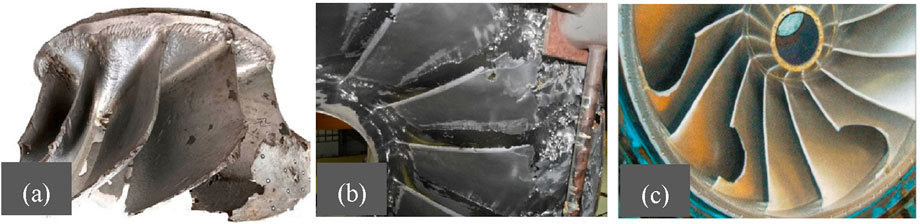
Figure 1. Sediment erosion in trailing edge of Francis turbines: (a) Trishuli Hydropower plant, Nepal (b) Kalidandaki Hydropower Plant, Nepal (c) Nathpa Jhakri Plant, India (Thapa et al., 2015; Sapkota et al., 2022; Sharma, 2010).

Another type of fault found in the runner is breakage due to fatigue loading and high-pressure fluctuations produced by rotor-stator interaction. Past studies suggest that cracks initially grow at a slow rate but increase significantly only after the onset of severe cycle fatigue (Avellan, 2000; Gagnon et al., 2012). Therefore, detecting cracks before the onset of high-cycle fatigue is both crucial and challenging due to the nature of their growth.

The flow inside the turbine is incorporated with instabilities and transients, which is more pronounced during deep part-load conditions. Large vibrations are produced in the machines due to these fluctuations (Zhao et al., 2020). Erosive cavitation in the runner can be detected by utilizing high-frequency acceleration signals from the turbine bearing (Valentín et al., 2018). Vibrations caused by abnormal operation and early-stage damage might remain undetected until they lead to significant damage in the turbine (Gagnon et al., 2012). Several common damages in hydraulic turbines are caused by vibration amplitudes at the rotational frequency, such as runner obstruction and damaged components (Egusquiza et al., 2011). The amplitude of the rotational frequency increases as associated damage appears (Vashishtha and Kumar, 2022).

Vibration monitoring is typically conducted on machinery such as turbines, pumps, and fans, which consist of several rotating parts like bearings and gearboxes (Tung and Yang, 2009). In one study, measurements were made in the axial direction as well as 90° apart in the vertical and horizontal directions (perpendicular to the shaft axis) for horizontal shaft machines (Egusquiza et al., 2018). Peak frequency shifts were less pronounced than peak amplitude shifts, with the trend of increasing amplitude shifts noticeable as the crack or fault progressed away from the hub (Gillich et al., 2015; Awadallah and El-Sinawi, 2020). The physical, geometrical, and boundary conditions also affect the vibration signature of the structure (Awadallah and El-Sinawi, 2020). A higher amplitude of vibration at harmonics of the fundamental frequency (1X) indicates faulty conditions such as unbalance, misalignment, and a bent shaft. However, misalignment issues and bent shafts typically cause strong vibrations in the 2X order synchronous frequency as well (Betta et al., 2002; Patel and Darpe, 2009; Adams, 2009).

In condition monitoring, signal processing techniques are crucial as they examine and establish the relationship between input data such as vibration, sound, and current signals and the damage in tools and machines (Mohanraj et al., 2020). Frequency spectrum analysis is advantageous because it shows how much of a signal exists within a given frequency band, whereas time-domain analysis only reveals changes in a signal over time. This makes frequency spectrum analysis ideal for signals with more non-stationary characteristics (Srinivasan and Eswaran, 2005). Vibration signature analysis is an effective technique for identifying and tracking machine faults, with levels of damage in tools and machines clearly indicated by shifts in the acceleration spectrum and changes in magnitude (Rmili et al., 2006). Sensors play critical role in condition monitoring, providing real-time data for predictive maintenance. However, sensor faults such as bias errors, gain faults and drift faults can lead to inaccurate diagnostics. Recent advancements in sensor-based fault diagnosis integrate AI-driven models that enhance accuracy of fault detection and isolation (Chauhan et al., 2024). Despite the advancements in ML and Senosr-based fault detection, challenges remain in data availability, model interpretability and adaptability to real-world environments. High-dimensional sensor data require efficient feature selection techniques, and deep learning models often lack transparency, making them difficult to interpret for industrial applications (Vashishtha et al., 2025).

This study aims to predict faults in a locally manufactured Francis runner by analyzing the frequency spectrum of the runner in both healthy and faulty conditions. A uniaxial accelerometer is placed at the turbine bearing to capture the shaft amplitude and its harmonics. Fast Fourier Transform (FFT) and Wavelet Transform along with EMD algorithm are applied to analyze the frequency components of the vibrational signal.

2 Experimental setup

The experimental setup consists of a Francis Test Rig, as shown in Figure 2. The rig features a main motor that pumps hydraulic fluid into the turbine and has a power capacity of 11 kW. It can produce up to a 36-m head with a discharge of 23.33 L/s. The pump is controlled using a Variable Frequency Drive (VFD) to achieve the required head and flow rate.

Figure 2

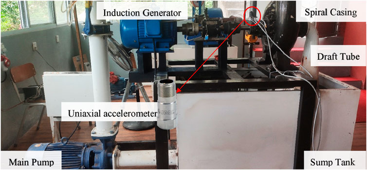
Figure 2. Experimental Francis turbine test rig.

Similarly, the rig includes a sump tank to store the hydraulic fluid, which circulates from the main pump through a pipe into the turbine and exits from the draft tube back into the sump tank. The major components of the test rig include the Francis turbine, spiral casing, draft tube, turbine shaft, and induction generator. The speed of the induction generator is also controlled using another VFD, and it has a power capacity of 3 kW. To maintain the position of the draft tube, the turbine components and generator are located above the sump tank.

For measuring the pressure, two absolute pressure sensors are used: one at the inlet of the turbine and the other at the outlet of the runner. The flow through the pipe is measured using an ultrasonic flowmeter, and the rotational speed of the turbine shaft is determined using an optical sensor. A uniaxial accelerometer is installed at the top of the turbine bearing to capture the radial vibrational signal. The data acquisition devices are from National Instruments, and the data acquisition program is developed in LabVIEW. The data acquisition rate is 12,000 samples per second for the vibration sensor and 2,000 samples per second for the pressure and rotational speed sensors. The data were acquired for each operating point for a duration of 12 s. Repeatability tests were conducted to ensure the repeating nature of the result. The specifications of the sensors and devices used during the experiments are listed in Table 1.

Table 1

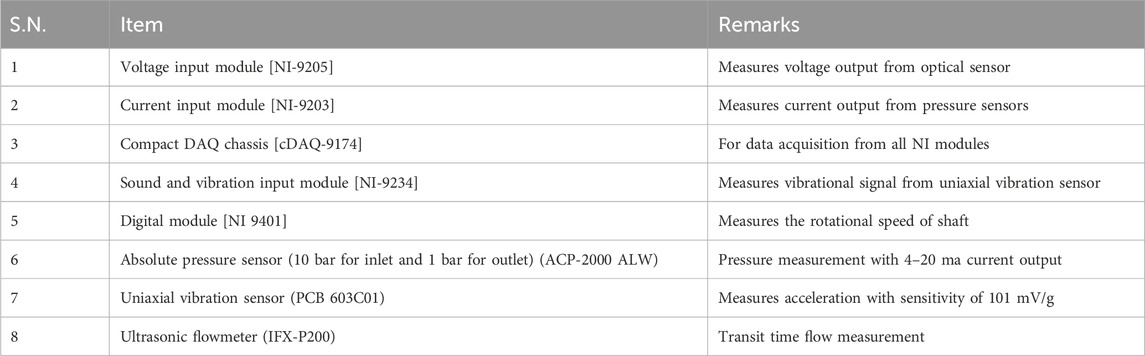
Table 1. Specifications of sensors and devices.

A locally manufactured Francis turbine (Figure 3, with a design head of 12 m and a design flow of 32 L per second, was selected as the test specimen for the experiment. The detailed design specifications of the Francis turbine are listed in Table 2. The turbine has ten blades and is optimally designed to operate at 2250 RPM.

Figure 3

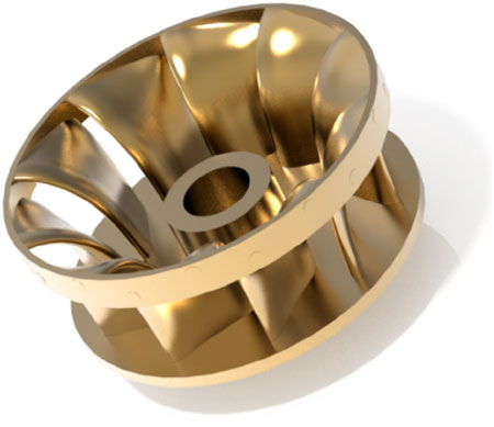
Figure 3. 3D model of locally manufactured Francis turbine.

Table 2

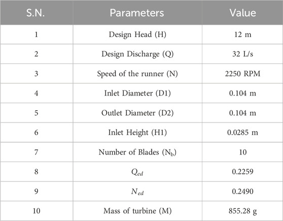
Table 2. Design specification of Francis turbine.

2.1 Experimental test cases

In this experiment, there are three main test cases referred to as Case One, Case Two, and Case Three. When the turbine operates in the absence of hydraulic flowing fluid, the cases are abbreviated as Case One Dry, Case Two Dry, and Case Three Dry. When the turbine operates in the presence of hydraulic flowing fluid, the cases are abbreviated as Case One Wet, Case Two Wet, and Case Three Wet. In the wet condition, a constant head of 4 m was maintained for all operating speeds. In all of the dry cases, the sump tank was kept empty, while in the wet cases, it was filled with water as the hydraulic fluid.

In a real scenario, when there is erosion in the turbine components, the overall mass of the turbine is reduced, which affects its balance. The trailing edge of the turbine blade is the most affected part due to erosion, as shown in Figure 1. To replicate this scenario, the blades at the trailing edge would need to be removed. However, removing the blade could damage the original turbine and make it difficult to repeat the experiment. To address this issue, faults in the turbine are induced by adding masses on the top of the turbine blades. Cyanoacrylate adhesive is used to glue the added masses to the turbine blades, and the masses are removable if necessary.

2.1.1 Case one

This case represents the normal condition of the turbine, with no induced faults. It is considered the reference signature case for comparison of the vibrational signals with the other cases.

2.1.2 Case two

In this case, a fault is induced by adding a mass to the top of the turbine blade, as shown in Figure 4a. The weight of the single mass added is 35 g.

Figure 4

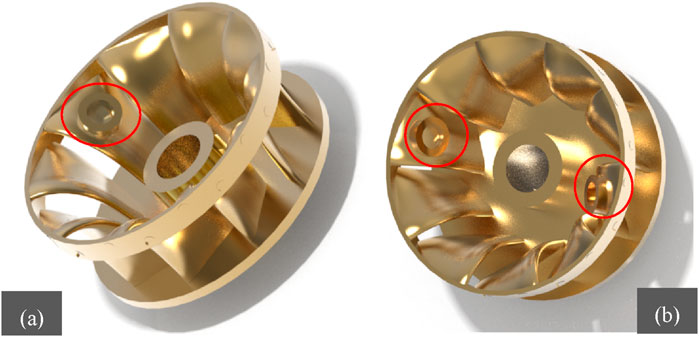
Figure 4. (a) Fault induced on single blade of a turbine and (b) Fault induced on two blades of a turbine.

2.1.3 Case three

Similar to Case Two, another mass is added to the top of the turbine blade, as shown in Figure 4b. The added mass has the same weight of 35 g and is placed on the opposite blade of the previously added mass.

2.2 Signal de-noising and wavelet transform process

Signal de-nosing is an important process in various vibrational applications including turbine signal analysis. In this study, the Empirical Mode Decomposition (EMD) de-noising algorithm was adapted to de-noise the vibrational signal acquired from the accelerometer. The EMD de-noising method was first introduced by Huang in 1998 for analyzing non-linear and non-stationary signals. The EMD algorithm decomposes the signal into intrinsic mode functions (IMFs), removes the noise from the signal by analyzing each of the IMFs components using the threshold technique, and reconstruction of signal after noise removal (Huang et al., 1998). The algorithm was improvised and applied by Dao et al. (2023) to de-noise the acoustic vibration signal of the hydro turbine to determine the frequency spectrum of water flowing with and without sediment load.

Fourier analysis is an effective tool to visualize the vibrational signal, decomposing the signal to identify frequency components. However, it is unable to provide the time when a particular frequency has occurred due to poor time localization (Alan et al., 1999). Due to this limitation, wavelet transform was adapted to better visualize the frequency components of a signal in the time frequency domain. Wavelet transform is accompanied by signal de-noising process.

The wavelet transform has been defined as a powerful computational tool that is popular for analyzing the characteristics of a signal and decomposes the signal into different scales which has better visualization in the both time and frequency domains (Daubechies, 1990). The overall concept of wavelet transform is the use of wavelet functions simply called wavelets which grow and decay in a limited time within a localized time-frequency domain to analyze the transient and non-stationary signals with a wide range of applications like signal processing, image processing, data compression, pattern recognition, etc. (Graps, 1995; E W and Chui, 1993).

$r_i\left(IMF,x\left(t\right)\right)=\frac{Cov\left(IMF,x\left(t\right)\right)}{\sqrt{Var\left[{IMF}_i\right]Var\left[x\left(t\right)\right]}}(1)$

In this study, after applying the EMD algorithm and generating IMFs, the correlation coefficient (Equation 1) of IMFs suggested by Dao et al. (2023) has been calculated to remove the noisy IMFs and signals were reconstructed to perform the Morlet wavelet transform. The outstanding value of the correlation coefficient acts as a critical point and IMFs before the critical correlation coefficient are considered to be noisy IMFs which are excluded from the signal. Morlet wavelet (Equation 2) is considered to be the best among the other wavelets for performing fault diagnosis and vibrational analysis of a signal. The wavelet was named in the name of Jean Morlet which combines the complex sine function with the Gaussian window and is very effective for analyzing the oscillatory behavior in signals (Grinsted et al., 2004; Goupillaud et al., 1984).

$\mathrm{\psi }\left(\mathrm{t}\right)=e^{\mathrm{i}{\mathrm{\omega }}_{0}t}{e}^{-t^2/\left(2{\mathrm{\sigma }}^2\right)}(2)$

Where, ψ(t) is the Morlet wavelet, ${\mathrm{\omega }}_0$ is the central frequency of the wavelet and σ is the standard deviation of the Gaussian window.

The EMD de-nosing process decomposes original signal into IMFs (see Figure 5) and correlation coefficient (Equation 1) was calculated for each of the IMFs. The IMFs before the outstanding correlation coefficient are considered to be noise and ignored to reconstruct the de-noised signal to perform wavelet transform process. A complex Morlet wavelet named ‘cmor1.5-1.5’ which is considered to be useful for sinusoidal signals was used to analyze signal’s time frequency characteristics, where the algorithm computes continuous wavelet transform coefficients. The results were compared in the form of scalogram plots.

Figure 5

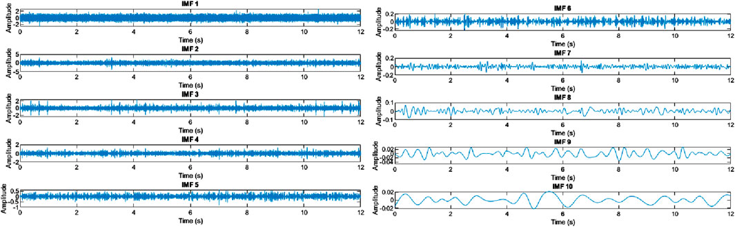
Figure 5. IMF decomposition of the vibrational signal using the EMD algorithm.

3 Result and discussions

The Fast Fourier Transform (FFT) algorithm was used to analyze the vibrational signal around the turbine bearing. FFT is one of the most efficient algorithms used to obtain the frequency components of a time-domain signal. (Cooley et al., 1969). Figure 6 shows the frequency spectrum of the vibrational data acquired at a rotational speed of 600 RPM under the Case One Wet condition. The amplitudes of the fundamental frequency (10 Hz) of the shaft and its harmonics (20, 30, 40, 50, 60) are the frequencies of interest for this specific speed and can be visualized in the graph. It also includes the vibrational frequency around 24 Hz, which corresponds to the frequency of main pump in operation. While comparing this plot with the FFT plot at dry condition, the presence of sub harmonic components can be seen in wet condition while it is not visible at the dry condition. This might be the vibrations due to the flowing fluid, resulting in various fluctuations.

Figure 6

Figure 6. Frequency spectrum of vibration data at 600 RPM (Case One Wet).

Similarly, for other test cases and operating speeds, the amplitude of the fundamental frequency and its harmonics were determined using FFT, referenced to the speed of the shaft. The speed of the shaft ranges from 7 to 16 Hz (420–960 RPM) for both dry and wet conditions. After determining the amplitudes of the shaft frequency, graphs were plotted for both dry and wet conditions with all test cases, as seen in Figures 7, 9.

Figure 7

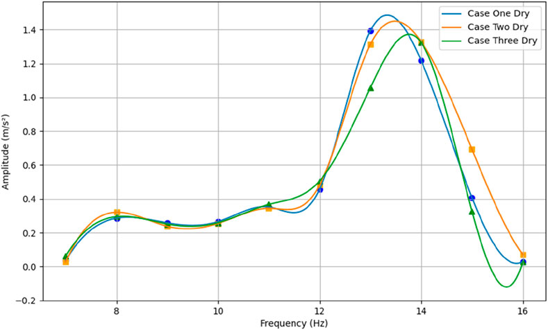
Figure 7. Vibrational amplitudes for fundamental frequency in dry condition.

While analyzing the result for dry condition (Figure 7), overlapping amplitudes can be observed between 7 and 12 Hz, followed by a peak in amplitude around the 12–14 Hz frequency, and a sharp decrease in amplitude after 14 Hz for all test cases. The peak amplitudes of 1.484, 1.449, and 1.371 m/s² can be seen in decreasing order as the faults increase, at frequencies of 13.36, 13.45, and 13.72 Hz for Case One Dry, Case Two Dry, and Case Three Dry, respectively. These frequencies can be referred to as the resonant frequencies, as they experience peaks due to the application of external forces. According to the literature, resonance occurs in a system when the excitation frequency matches its natural frequency, which depends on the system’s mass, stiffness, and geometry (Kraige, 2015; Singiresu, 2010).

Figure 8 shows the comparative plot of vibrational amplitude for the fundamental frequency in the dry condition. The dry condition is defined as the state when no hydraulic fluid is flowing through the turbine components, with experiments conducted under normal turbine conditions (emptying and filling the sump tank), abbreviated as Case Empty and Case Filled, respectively. The result of Case Filled shows almost a 1000% reduction in the vibrational resonant amplitude peak compared to Case Empty. This indicates that vibration is absorbed when the sump tank is filled with hydraulic fluid.

Figure 8

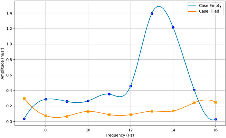
Figure 8. Vibrational amplitudes for fundamental frequency in dry condition.

Similarly, while performing experiments in the wet condition (Figure 9), the results are comparable to the dry condition. The resonating peak has shifted to 10 Hz, while it was about 13.5 Hz in the dry condition. The peak amplitudes for Case One Wet, Case Two Wet, and Case Three Wet at the resonating frequency of 10 Hz were obtained as 0.429149, 0.362469, and 0.521942 m/s², respectively. The amplitude of vibration is lower in the wet condition (0.429149 for Case One Wet) compared to the dry condition (1.484 for Case One Dry) for all the cases. When comparing Case One Wet (normal) and Case Two Wet (faulty), the resonating peak amplitude decreases in Case Two Wet. In contrast, in Case Three Wet (faulty), the resonating peak amplitude is the highest.

Figure 9

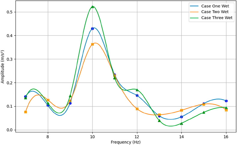
Figure 9. Vibrational amplitudes for fundamental frequency in wet condition.

The scalogram plot is useful to visualize the amplitude variations of a signal in the both time and frequency domain. Figures 10, 11 represent the scalogram plot for wavelet transform result of faulty cases, i.e., dry and wet. Referring to Figure 7, wavelet transform algorithm for dry condition has been applied to visualize the transient behavior of signal. Figure 10 is the scalogram plot for the Case Three Dry (faulty) in which the turbine is operated at 13 Hz, and it shows the dominant frequency components which is concentrated at 13 Hz and aligns with the FFT result. The plot shows clear and consistent energy distributions at the operating frequency over time.

Figure 10

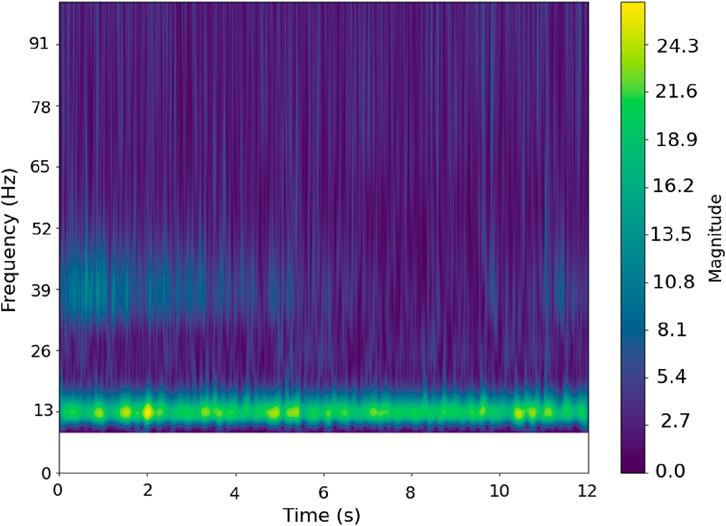
Figure 10. Scalogram plot for case three dry.

Figure 11

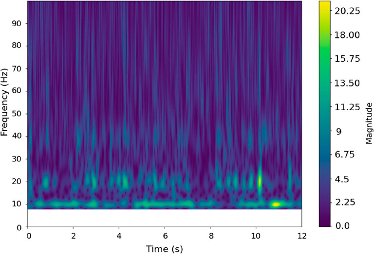
Figure 11. Scalogram plot for case three wet.

Similarly, with reference to Figure 9, scalogram plots for wet condition has been generated to visualize the signal in time frequency domain. Figure 11 is the plot for Case Three Wet (faulty) in which turbine’s operational frequency is 10 Hz and is the dominating frequency component in the scalogram plot as well. Overall concentration of the energy is at 10 Hz and is consistent along the time domain. Comparing the plot with dry case, the amplitudes of the dominating frequency in wet case is low and it aligns with the FFT result in Figure 9. In both of the plots, there is a presence of weaker but visible components at the multiple of turbine’s frequency.

4 Conclusion

The study aims to predict turbine faults by applying the frequency transform algorithm and signal de-noising followed by wavelet transform algorithm to visualize vibrational time series data. The turbine faults are self-induced by adding masses to the top of the turbine blades. The experiment revealed that the turbine fault (adding masses) primarily affects the amplitude of the peak resonating frequency, with minimal effect on the amplitudes of other frequencies. The induced fault in the turbine can either increase or decrease the amplitude of the peak resonating frequency. In the dry condition, as the severity of the fault increased, the amplitude of the peak resonating frequency decreased from 1.484 to 1.371 m/s². In the wet condition, as the severity of the fault increased, the peak resonating frequency initially decreased from 0.429 to 0.3762 m/s², and then increased to 0.521 m/s² as the severity further increased. It can be concluded that turbine faults can be predicted by studying the amplitude of the resonating frequency.

While analyzing the results with the wavelet transform algorithm in scalogram plot, it aligns with the result of Fast Fourier Transform algorithm. In both dry and wet condition, there is clear and consistent energy distributions at the turbines operating frequency in Figures 10, 11. Also, the stronger amplitudes of turbine’s frequency can be seen in scalogram plot in dry condition compared to wet condition and it is the same with FFT result.

As suggested by the literature (Kraige, 2015; Singiresu, 2010), any changes in the mass of the system can alter the natural frequency of the system. In this experiment, when transitioning from dry to wet conditions, hydraulic fluid was added to the sump tank, causing the natural frequency of the system to shift from about 13.5 to 10 Hz, along with a decrease in the amplitude of the vibrational signal. Thus, any changes in the mass of the system can shift the resonating frequency.

Data availability statement

The original contributions presented in the study are included in the article/supplementary material, further inquiries can be directed to the corresponding authors.

Author contributions

PS: Data curation, Formal Analysis, Investigation, Methodology, Software, Writing–original draft, Writing–review and editing. SP: Formal Analysis, Investigation, Methodology, Writing–original draft, Writing–review and editing. RP: Investigation, Software, Writing–review and editing. SC: Formal Analysis, Funding acquisition, Project administration, Resources, Supervision, Validation, Visualization, Writing–review and editing. HN: Formal Analysis, Funding acquisition, Project administration, Resources, Supervision, Validation, Visualization, Writing–review and editing. BT: Formal Analysis, Funding acquisition, Project administration, Resources, Supervision, Validation, Visualization, Writing–review and editing.

Funding

The author(s) declare that no financial support was received for the research, authorship, and/or publication of this article.

Acknowledgments

This work is conducted as part of a Ph.D. study at the Turbine Testing Lab, Department of Mechanical Engineering, Kathmandu University. The research is assisted and supported by some key projects; EnergizeNepal project; FranSed project; TTL-Fault Project; and CMHydro project. The authors are highly indebted to all colleagues and staff working at Turbine Testing Lab for continuous help, support, and encouragement throughout the completion of this research.

Conflict of interest

The authors declare that the research was conducted in the absence of any commercial or financial relationships that could be construed as a potential conflict of interest.

Generative AI statement

The author(s) declare that no Generative AI was used in the creation of this manuscript.

Publisher’s note

All claims expressed in this article are solely those of the authors and do not necessarily represent those of their affiliated organizations, or those of the publisher, the editors and the reviewers. Any product that may be evaluated in this article, or claim that may be made by its manufacturer, is not guaranteed or endorsed by the publisher.

References

Adams, M. L. (2009). Rotating machinery vibration. Boca Raton: CRC Press.

CrossRef Full Text | Google Scholar

Alan, V. O., Ronald, W., and Schafer, J. R. B. (1999). Discrete-time signal processing. Prentice Hall.

Google Scholar

Avellan, F. (2000). Flow investigation in a Francis draft tube: the flindt project.

Google Scholar

Awadallah, M., and El-Sinawi, A. (2020). Effect and detection of cracks on small wind turbine blade vibration using special Kriging analysis of spectral shifts Measurement 151 107076.

Google Scholar

Betta, G., Liguori, C., Paolillo, A., and Pietrosanto, A. (2002). A DSP-based FFT-analyzer for the fault diagnosis of rotating machine based on vibration analysis. IEEE Trans. Instrum. Meas. 51, 1316–1322. doi:10.1109/tim.2002.807987

CrossRef Full Text | Google Scholar

Breeze, P. (2019). Hydropower power generation technologies. Elsevier, 173–201.

CrossRef Full Text | Google Scholar

Chauhan, S., Vashishtha, G., and Zimroz, R. (2024). Analysing recent breakthroughs in fault diagnosis through sensor: a comprehensive overview. A Compr. Overv. comput. Model. Eng. Sci. 141, 1983–2020. doi:10.32604/cmes.2024.055633

CrossRef Full Text | Google Scholar

Chitrakar, S., Neopane, H. P., and Dahlhaug, O. G. (2018). A review on sediment erosion challenges in hydraulic turbines sediment. Eng.

Google Scholar

Cooley, J. W., Lewis, P. A. W., and Welch, P. D. (1969). The Fast fourier Transform and its applications vol 12 engalewood cliffs. New Jersey: Prentice Hall, Inc.

Google Scholar

Dao, F., Zeng, Y., and Qian, J. (2023). A novel denoising method of the hydro-turbine runner for fault signal based on WT-EEMD. Measurement 219, 113306. doi:10.1016/j.measurement.2023.113306

CrossRef Full Text | Google Scholar

Daubechies, I. (1990). The wavelet transform, time-frequency localization and signal analysis. IEEE Trans. Inf. Theory 36, 961–1005. doi:10.1109/18.57199

CrossRef Full Text | Google Scholar

Egusquiza, E., Valero, C., Estévez, A., Guardo, A., and Coussirat, M. (2011). Failures due to ingested bodies in hydraulic turbines. Eng. Fail. Anal. 18, 464–473. doi:10.1016/j.engfailanal.2010.09.039

CrossRef Full Text | Google Scholar

Egusquiza, M., Egusquiza, E., Valero, C., Presas, A., Valentín, D., and Bossio, M. (2018). Advanced condition monitoring of Pelton turbines. Measurement 119, 46–55. doi:10.1016/j.measurement.2018.01.030

CrossRef Full Text | Google Scholar

E W, C., and Chui, C. K. (1993). An introduction to wavelets. Math. Comput. 60, 854. doi:10.2307/2153134

CrossRef Full Text | Google Scholar

Gagnon, M., Tahan, S. A., Bocher, P., and Thibault, D. (2012). The role of high cycle fatigue (HCF) onset in Francis runner reliability IOP. Conf. Ser. Earth Environ. Sci. 15, 022005. doi:10.1088/1755-1315/15/2/022005

CrossRef Full Text | Google Scholar

Gillich, G.-R., Maia, N. M. M., Mituletu, I.-C., Praisach, Z.-I., Tufoi, M., and Negru, I. (2015). Early structural damage assessment by using an improved frequency evaluation algorithm. Lat. Am. J. Solids Struct. 12, 2311–2329. doi:10.1590/1679-78251795

CrossRef Full Text | Google Scholar

Goupillaud, P., Grossmann, A., and Morlet, J. (1984). Cycle-octave and related transforms in seismic signal analysis. Geoexploration 23, 85–102. doi:10.1016/0016-7142(84)90025-5

CrossRef Full Text | Google Scholar

Graps, A. (1995). An introduction to wavelets. IEEE Comput. Sci. Eng. 2, 50–61. doi:10.1109/99.388960

CrossRef Full Text | Google Scholar

Grinsted, A., Moore, J. C., and Jevrejeva, S. (2004). Application of the cross wavelet transform and wavelet coherence to geophysical time series. Nonlinear process. Geophys 11, 561–566. doi:10.5194/npg-11-561-2004

CrossRef Full Text | Google Scholar

Huang, N. E., Shen, Z., Long, S. R., Wu, M. C., Shih, H. H., Zheng, Q., et al. (1998). The empirical mode decomposition and the Hilbert spectrum for nonlinear and non-stationary time series analysis. Proc. R. Soc. Lond. Ser. A Math. Phys. Eng. Sci. 454, 903–995. doi:10.1098/rspa.1998.0193

CrossRef Full Text | Google Scholar

Kraige, L. G. (2015). Meriam J L dynamics. Hoboken: Wiley.

Google Scholar

Mohanraj, T., Shankar, S., Rajasekar, R., Sakthivel, N. R., and Pramanik, A. (2020). Tool condition monitoring techniques in milling process — a review. J. Mater. Res. Technol. 9, 1032–1042. doi:10.1016/j.jmrt.2019.10.031

CrossRef Full Text | Google Scholar

Patel, T. H., and Darpe, A. K. (2009). Experimental investigations on vibration response of misaligned rotors. Mech. Syst. Signal Process. 23, 2236–2252. doi:10.1016/j.ymssp.2009.04.004

CrossRef Full Text | Google Scholar

Rmili, W., Serra, R., Ouahabi, A., Gontier, C., and Mecheri, K. (2006). Tool wear monitoring in turning process using vibration measurement. 5.

Google Scholar

Sapkota, P., Chitrakar, S., Neopane, H. P., and Thapa, B. (2022). Problem identification and condition monitoring status of Nepalese power plants. IOP Conf. Ser. Earth Environ. Sci. 1079, 012064. doi:10.1088/1755-1315/1079/1/012064

CrossRef Full Text | Google Scholar

Sharma, H. K. (2010). Power generation in sediment laden rivers: the case of Nathpa Jhakri. Int. J. Hydropower and Dams 17, 112–116. Available online at: https://www.hydropower-dams.com/articles/power-generation-in-sediment-laden-rivers-the-case-of-nathpa-jhakri/.

Google Scholar

Singiresu, S. R. (2010). Mechanical vibrations.

Google Scholar

Srinivasan, V., and Eswaran, C. (2005). Artificial neural network based epileptic detection using time-domain and frequency-domain features. J. Med. Syst. 29, 647–660. doi:10.1007/s10916-005-6133-1

PubMed Abstract | CrossRef Full Text | Google Scholar

Thapa, B. S., Dahlhaug, O. G., and Thapa, B. (2015). Sediment erosion in hydro turbines and its effect on the flow around guide vanes of Francis turbine. Renew. Sustain. Energy Rev. 49, 1100–1113. doi:10.1016/j.rser.2015.04.178

CrossRef Full Text | Google Scholar

Tung, T. V., and Yang, B.-S. (2009). Machine Fault diagnosis and prognosis: the state of the art. State Art Int. J. Fluid Mach. Syst. 2, 61–71. doi:10.5293/ijfms.2009.2.1.061

CrossRef Full Text | Google Scholar

Valentín, D., Presas, A., Egusquiza, M., Valero, C., and Egusquiza, E. (2018). Transmission of high frequency vibrations in rotating systems. Application to cavitation detection in hydraulic turbines. Appl. Sci. 8, 451. doi:10.3390/app8030451

CrossRef Full Text | Google Scholar

Vashishtha, G., Chauhan, S., Sehri, M., Zimroz, R., Dumond, P., Kumar, R., et al. (2025). A roadmap to fault diagnosis of industrial machines via machine learning: a brief review. A Brief. Rev. Meas. 242, 116216. doi:10.1016/j.measurement.2024.116216

CrossRef Full Text | Google Scholar

Vashishtha, G., and Kumar, R. (2022). Pelton wheel bucket fault diagnosis using improved shannon entropy and expectation maximization principal component analysis. J. Vib. Eng. Technol. 10, 335–349. doi:10.1007/s42417-021-00379-7

CrossRef Full Text | Google Scholar

Xu, J., Badola, R., Chettri, N., Chaudhary, R. P., Zomer, R., Pokhrel, B., et al. (2019). Sustaining biodiversity and ecosystem services in the Hindu Kush himalaya. 127, 165. doi:10.1007/978-3-319-92288-1_5

CrossRef Full Text | Google Scholar

Zhao, W., Egusquiza, M., Valero, C., Valentín, D., Presas, A., and Egusquiza, E. (2020). On the use of artificial neural networks for condition monitoring of pump-turbines with extended operation Measurement 163 107952.

Google Scholar