Oppositional chaotic artificial hummingbird algorithm on engineering design optimization

This paper proposes an enhanced-search form of the newly designed artificial hummingbird algorithm (AHA), named oppositional chaotic artificial hummingbird algorithm. The proposed OCAHA methodology incorporates the oppositional learning (OBL) in the population-initialization and at the ending event of each iteration for a faster convergence, and the chaos-embedded sequences of Gauss/mouse map to replace the random sequences of the three population-updating iterative stages of AHA, viz. guided, territorial and migration foraging to employ more diverse population for more solutional accuracy. The effectiveness of the method has been evaluated in two phases. OCAHA, the four state of the art algorithms, namely, PSO, DE, GWO and WOA, their recently developed effective variants, namely, SLPSO, MTDE, SOGWO and EWOA, and the inspiring optimizer AHA have been implemented on the 29 unconstrained CEC 2017 benchmark functions in the first phase. In the second phase, OCAHA has been verified on 10 challenging engineering cases, and compared with the concerned leading performances. Comprehensive analysis of the simulated outcomes using various statistical metrics and of the convergence profiles demonstrates that, the optimization ability of OCAHA on CEC 2017 is superior to all the comparing algorithms except MTDE. For engineering cases, OCAHA provides better searching performance, solution precision, robustness and convergence rate than all competing designs, and, on average, it has lowered the computational cost by 57.5% and 22.63% in term of function evaluations and the fitness objective by 2.4% and 0.23% in comparison to AHA and the chaotic version CAHA, respectively.

GRAPHICAL ABSTRACT

Highlights

• An oppositional-chaotic metaheuristic approach (OCAHA) applied on CEC 2017 test suite.

• Ten number challenging cases of engineering design optimization have been solved.

• OCAHA performance on CEC 2017 found satisfactory among its 9 competitors.

• Optimized engineering designs by OCAHA are better than previous studies.

1 Introduction

As the losses are inevitable during any energy transferring process of a real working system, it has always been an important concern for researchers to recover these associated losses to obtain more efficient system output, and in today’s world scenario of energy crisis, this is not limited to recovery and proper reutilization of these lost forms of energy, but extends to the optimum utilization of a number of different forms of non-conventional energy to meet the continuously increasing demand. Research and development always finds the new technological means to fulfill the existing needs at the affordable acceptance as well as to advance the existing modes of needs or requirements. The efficiency of any operational system is the integrated effect of all the individual functional unit efficiencies of the system and each component of each of these functional units or machines transfers the required motions individually or in integrated manner to develop and deliver the total output of the unit or machine. Among the several designing aspects to make an efficient, cost-effective and reliable working system to meet the high-speed and high-precision demands of modern times, design optimization of the geometry of some intricate-shaped machine components to ensure more smoothness and reliability in its functioning and of the various operational factors of some complex operational units to achieve the desired objectives has become a highly challenging area of research. In continuing the research work in this direction of research with more effective optimized designs, ten number of challenging cases of engineering design problems have been chosen in the present study for constrained design optimization.

Galileo’s (1,564–1,642) shape optimizing theory (Cajori, 1999) is the first literature in this context to formulate the structural inter-relation between the shape and the strength of a bent beam mathematically, and the theory identified the bent beam shape for its uniform strength. Subsequently, several great scientists came up with a variety of classical implementing methods in various working directions. Pareto’s (Kasprzak and Lewis, 2001) multi-objective optimization principle, Gerard’s analysis for weight minimizing of structures (compression) by linear programming (George, 1956), Schmit and Miura approximation for structural synthesis (Schmit et al., 1976), application of linear programming and branch and bound method (Wolsey, 1998) in production and transportation planning in industries, reliability-redundancy allocation problem (RRAP) problems solving by dynamic programming and implicit enumeration to optimize system reliability (Rajendra Prasad and Kuo, 2000), Lagrangian programming (relaxation and quadratic) techniques (Petcharaks and Ongsakul, 2007), and numerous other classical optimization methods had been formulated and effectively implemented in various optimization requirements. The major issues associated with these classical optimization methods are; these methods are mostly deterministic in nature, dependent on gradient-based information, and usually suffer from unbalanced exploratory-exploitative search motion and locally entrapment problem (Cheng and Prayogo, 2017; Gu et al., 2018).

In overcoming these issues of the traditional mathematics-based optimizers and to succeed with the continuously evolving technological challenges, optimizing experimentation in the recent past decades have been inclined to a new direction of optimization techniques, called metaheuristics. Operational simplicity, randomized initial solutions, easy parallel search processing, strong robustness ability in optimized results, etc., are the effective metaheuristic algorithmic qualities in optimizing a large variety of practical-world oriented problems. Using the randomly initialized set of population or solutions, all these metaheuristics proceed through their distinct algorithmic methodologies to reach the global or an approximation of the global solution for an optimization problem. Numerous metaheuristic techniques have been effectively implemented in solving the complicated cases of various working areas like, economy and trade (Rafi and Dhal, 2020), finance (El-Abbasy et al., 2020), process control (Wang Hongyang et al., 2021), management (Wang Xiuwang et al., 2021), image processing (Agrawal et al., 2022), industry processing (Om Prakash et al., 2022), structural and elementary machine designing (Awad, 2021), machine learning and neural network optimization (Aasim et al., 2022), and several other engineering and applied science requirements. Some recently approached metaheuristic techniques are feature selection (Taradeh et al., 2019), spam detection (Faris et al., 2019), parameter identification (Abbassi et al., 2019), image segmentation (Rodríguez-Esparza et al., 2020) and prediction (Qiao et al., 2020). Based on the different inspiring sources of natural phenomena, metaheuristic optimizing methods have been roughly categorized into four sections as follows: evolutionary algorithms (Jordán et al., 2022); swarm intelligent algorithms (Rajesh et al., 2021); algorithms inspired from the different events of science (physical and chemical) (Sun et al., 2021; Deng et al., 2021); and human behavioural activity-based optimizers (Yan et al., 2022).

The evolutionary-based optimization algorithms have been developed from the Darwin theory of evolution. These algorithms conceptualize some natural and biological evolutionary events of some distinct creatures, like selection, reproduction, combination, and mutation into the methodologies, where the global solutions are obtained through creating a new descendent inhering its parents properties for every next-generation involving the randomly selected current individuals as parents. Genetic algorithm (Holland, 1975) (Goldberg, 2006) is the pioneer and among the widely applied metaheuristic techniques in this category. Differential evolution method (DE) (Storn and Price, 1997), bio-geography-based optimization (BBO) (Simon, 2008) and several other effective processes come in this section. Migration and mutation are the two main operators of the BBO algorithm to perform search locally and globally respectively. This algorithm is simple and unique in its algorithmic design and possesses a faster pace towards convergence. Issues associated with the BBO algorithm are its poor search capability, local optima stagnation and mainly, the computational complexity (Zhang Xinming et al., 2020). In the swarm-structured metaheuristics, the different social activities within the swarms of various living creatures, and between the swarms members and their surroundings have been theorized to develop the optimizing methodologies. Self-organization, durability, information sharing ability among the multiple agents, easy parallel search processing, learning ability through the generation steps and design simplicity basically result in the efficient optimization search with this categorized algorithms. A large number of effective algorithms of this category have been formulated and utilized in a consistent mode, and still in the exploring phases of optimization research for new additions. Particle swarm optimization algorithm (PSO) is the benchmark and the most common technique of the group, proposed by Kennedy and Eberhart (Kennedy and Eberhart, 1995; Kennedy and Eberhart, 1997). PSO model was inspired by the foraging movements of birds swarms. This algorithm is characterized by its good convergence rate, but, for some high dimensional search spaces, it suffers from the issue of easy entrapment into the local optima, and to some extent, sensitive to its control parameters (Zhang et al., 2015). In the third category of metaheuristics, different invented theories of physics and chemistry have been conceptualised to develop the optimizing methodologies. Gravitational search algorithm (GSA) (Rashedi et al., 2009) is one of the widely used algorithms in this class, developed from the Newton’s Law of Gravitation. The algorithm big bang-big brunch (BBBC) (Osman and Eksin, 2006) from the universe evolution theory, chemical reaction algorithm (Khac Truong et al., 2013) from the observation on chemical reactions, and several other effective optimization techniques fall in this category. In human behavioural activity-based optimizers, various activities of our society and its immediate environment have been capitalized to develop the optimization methodologies. Harmony search (Lee and Geem) algorithm (HS) (Lee and Geem, 2005) is an algorithmic formulation of a musical procedure for determining the level of harmony. Teaching learning-based optimization algorithm (TLBO) (Venkata Rao et al., 2011) is an another effective optimization methods of the same kind, based on the two phases of a teacher-students classroom interactions. In the teacher’s phase, the students or the learners learn directly from their teachers, and during the students’ or learners’ phase, they exchange their knowledge and get benefited further. The above discussed algorithms are to introduce the each category of metaheuristics. Besides, an ample number of optimization techniques of each of the four categories have been effectively employed in solving the problems of a large variety of optimization areas.

The designing object of an efficient optimizing framework is to obtain the optimal optimization at an acceptable computing cost while ensuring simplicity in its implementation. But, in reality, most of these metaheuristic optimization techniques suffer from the issues of local optima entrapment, low and imbalanced convergence mobility, low quality solution precision, long and uncertain computational run and high computational complexity, especially for the high dimensional search spaces. As a transitional evolution of this research (optimization), a new practice of hybridizing two or more number of different optimization algorithm features had been developed to enhance the solving ability, and this technique is still in effective application in several challenging cases of optimization. A GWO variant, EEGWO (Wen et al., 2018) with exploratory enhancing mechanism to solve the high-dimensional search spaces of global optimization problems, a modified self-organizing hierarchical PSO variant, HPSO-TVAC (Ghasemi et al., 2019), a combined form of PSO and DE (Okulewicz and Mańdziuk, 2019) in solving the dynamic vehicle routing problem with continuous space are to mention some examples of recent hybridization approach of metaheuristics.

Application of chaos in the optimization methodologies is an another useful technique to enhance the search quality of an optimization process. Utilizing the randomness and sensitivity properties of chaos to the initial condition of an optimization process, a highly diverse population can be generated at the output and thereby reducing the locally entrapment issue and excite the search mobility of the process towards global convergence. Chaotic sine cosine operator in CSCWOA to improve the global search and to mobilize the local searching processes of original WOA (Liu and Li, 2018), chaotic dolphin swarm algorithm (CDSA) in optimizing high-dimensional spaces (Qiao and Yang, 2019), implementation of Gaussian mutation operator (GM) for population diversification at first and then utilizing chaos-enhanced localized search (CLS) combined with GM in the flame updating process for population diversification in the second stage to improve the local exploitation in CLSGMFO (Xu et al., 2019), and introducing chaos in the switching possibility between local (abiotic pollination) and global (biotic pollination) searches and applying incremental search strategy to intensify the motion in some modifications of FPA, $i.e$ flower pollination algorithm (Burcin Ozsoydan and Baykasoglu, 2021) are to mention some of the effective works in the recent past on chaotic optimization. Stochasticity, ergodicity and the non-periodic complex characteristics have found a vast applicability of the different chaotic maps for a huge variety of optimization requirements.

The opposition-based learning rule (OBL) is an another widely employed search-enhancing technique to develop a greater variety in the population to achieve more effectiveness and thoroughness in the search process for a faster convergence for an optimization process. Tizhoosh (Hamid, 2005) introduced the OBL rule in the field of machine intelligence. The concept of involving a randomized population and its opposite population instead of two randomized (independent) population sets basically ensures more convenience in the search process to converge into the desired optimum solution in an unknown space (Rahnamayan et al., 2008) of optimization. Generally, during the earlier stages, when the current population (randomized) may probably at far away from the desired optimum solution, applying the OBL (opposite population) rule can move the search closer to the target and can save the search effort, and when the current population (randomized) already reaches in the close vicinity of the target in the later iterations, this rule may generate unnecessary exploratory search in the optimization. However, optimum utilization of this rule to accelerate the convergence mobility of an optimizing process is a matter of extensive research (Hamid, 2005). In an opposition-based optimization process, during initialization, both randomly initialized set and the opposite set of population or solutions are simultaneously processed to sort out the better population as the current set of solutions. These current population or solutions are updated in the 1st iteration stages of an optimization algorithmic process, and after obtaining the updated set, an opposite (set) of the updated set is determined and then both (sets) are combined, and then again the better population or better solutions are sorted out from this combined set as the current population or the current solutions for the next (2nd iteration) update, and continues to update in the same way up to the stopping criteria of maximum iterations. Application of OBL on the chosen weakest $(\omega )$ wolves using Spearman’s correlation coefficient to prevent excessive exploration and to enhance the rate of convergence of grey wolf optimizer (GWO) (Dhargupta et al., 2020), utilizing OBL rule together with a novel updating approach and other search enhancers in mobilizing the convergence and in improving the solutional precision of original equilibrium optimizer (Fan et al., 2021), using multi-leader wandering around search strategy (MLWAS) to enhance the global exploratory search, random high-speed jumping strategy (RHSJ) to better the local exploitation, and an adaptive lens opposition-based learning strategy to escape from local entrapment in an improved arithmetic optimization algorithm variant, called LMRAOA (Zhang et al., 2022) in solving numerical as well as engineering problems, etc., are some recently reported works utilized the OBL rule.

Design optimization of the machine components of different engineering systems has become a highly competitive area of optimization research. Minimizing the system mass or volume, maximizing the system work output and efficiency, minimizing the different cost aspects, minimizing the energy or power loss and many more developing areas of engineering design optimization are in practice. We highlight a few of the most current engineering design optimization works. Zhang Yiying et al. (2020). merged the TLBO feature of fast convergence with the global optimization strategy of neural network algorithm to developed TLBO-NNA, a hybrid method, and obtained effective solutions for four benchmark engineering components, viz., WBD, tension/compression spring, PV and the SR problem. Venkata Rao and Pawar (2020). implemented three number Rao algorithms for constrained optimization of ten number mechanical engineering system components and obtained better designs for all the cases. Jena et al. (2022). utilized material generation (MGA) and sunflower optimization (SOA) algorithms and the Taguchi technique to optimize a multi-objective problem for maximizing output power and system efficiency for a speed reducer (industrial) by controlling its three system variables, viz, the electric motor speed, lubricant viscosity and the current intensity. In (Pavanu Sai and Rao, 2022), the powerful exploratory characteristic of NSGA II together with the strong exploitative ability of PSO has been utilized for a shell-tube heat exchanger (STHE) cost minimization. An automatic optimization method (Guan et al., 2022) integrating fluid-structure interaction (FSI), the NSGA-II algorithm, and design of experiment (DoE) to upgrade the design quality and the efficiency of a propeller, and obtained better results. A recently reported bio-inspired optimization algorithm, starling murmuration optimizer (SMO) (Zamani et al., 2022) proposing a dynamic construction (multi-flock) and three new searching approaches, viz, separating, diving, and whirling search has been implemented on various benchmark test functions and some classical optimization cases of mechanical engineering system like, design of tension/compression spring, PVD, design of three-bar truss, WBD, gas transmission compressor design (GTCD), HTBD, design optimization of industrial refrigeration system and MDCBD problem, and the optimized designs have established the algorithm performance superiority. In reviewing the application of machine learning (ML) to additive manufacturing, a recently reported work (Vashishtha et al., 2024) has emphasized how ML may help with issues including design, material selection, and process flaws. Design optimization, process monitoring, and product quality are all enhanced by machine learning (ML), which also highlights the significance of data protection and a cooperative approach with human operators for successful deployment. In a recent study (Chauhan et al., 2024), a denoising filter that uses mountain gazelle optimization (MGO) to improve machinery signals’ slight non-stationarities was introduced. Through the improvement of kurtosis, signal-to-noise ratio (SNR), and impulsiveness extraction, the filter successfully lowers interference from the environment and other items of machinery. Acoustic and vibration indications from a malfunctioning belt conveyor system have been used to verify its functionality. A denoising filter that optimizes spectral kurtosis using the flow direction algorithm (FDA) has been developed by another study (Vashishtha et al., 2025) in the same direction. This filter boosts modest non-stationarities. To efficiently recover impulsive components from signals with complicated time-frequency structures, the filter has been designed using the optimal spectral kurtosis, free from thresholding circumstances.

No Free Lunch theorem (Wolpert and Macready, 1997) says that, a single optimization algorithm cannot solve all the optimization problems. In other words, if a particular optimizer is capable to solve a particular optimization problem successfully, there is a high probability of unsatisfactory performance by this algorithm in dealing with other problems. The theory consistently inspires the researchers to invent new methodologies as continuous algorithmic reforms and development in this domain of research. Besides, achieving more balanced exploratory-exploitative search motion, reducing the control parameters usage, and the other existing issues experienced with the performance of all the metaheuristic techniques are the probable reasons to explore this field in a continuous mode. Artificial hummingbird algorithm (Zhao et al., 2022; Sultan Yildiz et al., 2022; Wang et al., 2022) is a newly established swarm intelligent optimizer. The three flower-nectar eating activities of natural hummingbirds via a superior quality memory updating practice by themselves, named, visit table, and with the sufficient utilization of their three distinct flying skills have been conceptualized in the three population-updating policies of AHA methodology. The concept of utilizing these three hummingbird flying patterns in their three foraging events via visit table ensures an effective exploration-exploitation in the search characteristic of the AHA optimization process. In the proposed OCAHA methodology, the OBL rule with elitism has been implemented in the initialization stage, after that, the random sequences have been replaced by the chaotically generated sequences by the one-dimensional chaotic map, Gauss/mouse during the population-updating stages of every iteration, and then, at the ending of each iteration, again the OBL rule has been implemented to achieve more optimization accuracy at a faster convergence. This study evaluates OCAHA in two phases of simulation. In the first phase, OCAHA and its chosen competitors have been implemented on 50 and 100 dimensional sets of the CEC 2017 unconstrained functions, and in the second phase, ten challenging engineering cases have been solved using the proposed technique.

The work’s foremost contributions are:

a. An oppositional-chaotic based metaheuristic optimization approach is made by incorporating the OBL rule and the chaotic sequence of the Gauss/mouse map into the AHA algorithmic structure to apply on the unconstrained benchmark functions of CEC 2017 test suite and ten number of challenging cases of engineering design optimization.

b. More solutional accuracy and a faster rate of convergence on the majority of the test cases have been identified as the effects of the incorporated chaos-influenced sequence and the oppositional rule respectively.

c. A thorough analysis of the simulated outcomes on CEC 2017 has been conducted using various statistical measures, tests and convergence profiles to assess OCAHA’s overall performance in comparison to the 9 competing algorithms including AHA. Overall, OCAHA has been found to be superior to all the comparing methods except MTDE.

d. The OCAHA optimized results on engineering cases have been statistically assessed with those of the considered competing algorithms to validate the performance superiority of the proposed algorithm. OCAHA, on average, achieved 57.5% and 22.63% improvement in the computational cost $\left(\text{FE}\right)$ and 2.4% and 0.23% in the fitness objective (BestΨ(x→)_min) in comparison to CAHA and AHA, respectively.

The rest of the study is arranged as follows: Section 2 reviews the AHA methodology, the OBL rule and the chaotic maps, and proposes the oppositional chaotic artificial hummingbird algorithm (OCAHA), section 3 describes the CEC 2017 unconstrained benchmark functions and the engineering problems, section 4 contains simulation results analysis for both CEC 2017 functions and engineering cases, and finally, section 5 concludes the study.

2 Algorithmic methodologies

2.1 Artificial hummingbird algorithm (AHA)

This algorithm (Zhao et al., 2022; Sultan Yildiz et al., 2022; Wang et al., 2022) is a newly proposed swarm-based optimizing method, that develops the different foraging (flower nectar) intelligence of hummingbirds from the different sources of flowers as their target foraging sources. The individual flowers ($i.e$ the individual qualities and contents of flower nectar) of a source, rate of feeding, and the time since the last foraging a source are the basic foraging requirements, that a hummingbird follows to identify its target source from a set of different sources. In AHA, each source is assumed to have same number and same kind of flowers for simplifying the method. A food source has been considered as an individual population or a solution vector, and the feeding rate from the source represents the corresponding objective fitness value. When there is a population of hummingbirds and a number (set) of food sources, each bird can recall its most recent foraging visit to each source. After foraging at their target source, each one of them informs the other members of the population of their last foraging visit, $i.e$ the position and the rate of feeding of the target source. Visit table represents a unique memory-updating exercise by natural hummingbirds during their food foraging movements. Visit table provides the updated or current position value, $i.e$ the current visit level value to each food source of a set for each hummingbird of a population, that directs the hummingbirds to select and move towards their target food source among the available sources of the set. The visit level value of a food source for a hummingbird indicates the length of time from the last eating (visiting) at the source by the bird. Therefore, if a source shows the longest unvisited time or the highest visit level value for a particular hummingbird in a population, it actually represents the best foraging source, i.e., the target source for the hummingbird to forage. If the visit table indicates a number of food sources with same highest visit level for a particular hummingbird, then the hummingbird targets the source that has the best rate of feeding. When a hummingbird visits its target food source, its visit level value becomes zero, and simultaneously the visit levels of all the other sources get updated with an increment of one for this particular hummingbird. In the visit table, visit level values of the relevant food sources must be updated following each updating event during each generation or iteration of the algorithm process. In this way, the target source selection and then performing the three intelligent food foraging events by sufficiently utilizing the three unique flying skills of natural hummingbirds have been mathematically structured in the AHA methodology to induce an effective search behaviour throughout a problem space of optimization. This section reviews the AHA algorithm framework by randomized initialization of population and the equational descriptions of the three hummingbirds’ flower-nectar foraging strategies, namely, guided, territorial and the migrating strategy as the updating events during each iteration, the opposition-based learning rule OBL, the chaos property, and then provides the steps to implement OCAHA.

2.1.1 Initialization

For a set of $w$ food sources and a population of $w$ hummingbirds, initialized population is;

$x_u=low+r.\left(up-low\right)u=1,\dots \dots ,w(1)$

where, $r$ is the random number, $r\in [0,1]$, $up$ is the upper and $low$ is the lower limits for a $f$-dimensional optimization space, and $x_u$ is the expression for the $u^{th}$ source’s initialized (randomized) position.

The initialized visit table positions are;

$\begin{array}{c}\hfill {VT}_{u,v}=\left\{\begin{array}{c}0ifu\ne v\hfill \\ null\text{u}=v\hfill \end{array}\right.\end{array}u,v=1,\dots ,w(2)$

where, $u=v$ means the same position of $v^{th}$ source and $u^{th}$ hummingbird, $i.e$ the $u^{th}$ hummingbird is currently visiting at the $v^{th}$ source for nectar eating, and $u\ne v$ or ${VT}_{u,v}=0$ is the $v^{th}$ food source position, which has just been searched by the $u^{th}$ member (bird) in the ongoing $i.e$ current generation, and following this food foraging occurrence, the other sources’ positions (visit levels) for this $u^{th}$ hummingbird get updated with an increment of 1.

2.1.2 Guided foraging

In this strategy, a hummingbird identifies its target that has the maximum or top positional value in the visit table, and if there exist a number of food sources with same highest positional value, the hummingbird targets the source with the best rate of feeding, $i.e$ with the lowest rate (for objective minimization) or with the highest rate (for objective maximization) from these sources. After finalizing the target source, the hummingbirds utilize their three natural flying movements, $i.e$ axial, diagonal and omnidirectional fly sufficiently to reach the target for the necessary feeding. A direction switch vector $I$ has been included here to regulate these three flying movements to ensure the optimum movement during each of the three food foraging events.

For a $f$-spaced (dimension) optimization, the direction vector $I$ for the axial flying motion is;

$\begin{array}{c}\hfill {I_u}^{\left(i\right)}=\left\{\begin{array}{c}1ifi=randi\left(\left[1,f\right]\right)\hfill \\ 0else\hfill \end{array}\right.\end{array}i=1,\dots ,f(3)$

Direction switch vector for the diagonal flight skill is;

$\begin{array}{c}\hfill {I_u}^{\left(i\right)}=\left\{\begin{array}{c}1ifi=R\left(j\right),j\in \left[1,k\right],R=randperm\left(k\right)\hfill \\ \text{and}k\in \left[2,\left\{r_1.\left(f-2\right)\right\}+1\right]\hfill \\ 0else\hfill \end{array}\right.\end{array}i=1,\dots ,f(4)$

Direction vector for the omnidirectional flight is;

${I_u}^{\left(i\right)}=1i=1,\dots ,f;u=1,\dots ,w(5)$

where, $randi([1,f])$ stands for generating a random integer from 1 to $f$, $randperm(k)$ is to create a randomized permutation of integers from 1 to $k$, and $r_1$ is the random number producer in $[0,1]$.

When a hummingbird resides at its target position, the other food sources are updated with their new visit level values, which results in developing a candidate food source in the process.

A candidate position (source) during the guided search foraging is developed as;

$y_u\left(t+1\right)=x_{u,TAR}\left(t\right)+s_1.I.\left(x_u\left(t\right)-x_{u,TAR}\left(t\right)\right)(6)$

$s_1\sim N\left(0,1\right)(7)$

here, $x_u(t)$ is the $u^{th}$ source’s position at time $t$, $i.e$ the current position, $x_{u,TAR}(t)$ represents the $u^{th}$ hummingbird’s target (source) position (at $t$), where the $u^{th}$ hummingbird is intending to visit, and the guided factor denoted by $s_1$ is defined by the normal distribution $N(0,1)$, where the mean and standard deviation are, respectively, 0 and 1.

The position of the $u^{th}$ source is updated as;

$\begin{array}{c}\hfill x_u\left(t+1\right)=\left\{\begin{array}{c}{x}_u\left(t\right)\mathrm{\Psi }\left(x_u\left(t\right)\right)\le \mathrm{\Psi }\left(y_u\left(t+1\right)\right)\hfill \\ y_u\left(t+1\right)\mathrm{\Psi }\left(x_u\left(t\right)\right)>\mathrm{\Psi }\left(y_u\left(t+1\right)\right)\hfill \end{array}\right.\end{array}(8)$

where, $\mathrm{\Psi }(.)$ represents the corresponding fitness function values. Equation 8 implies that, if a candidate flower-nectar foraging source provides better food rate, $i.e$ if $\mathrm{\Psi }(y_u(t+1))$ (solution) is less (for objective minimization and vice versa) than that of the current food source, $i.e$. $\mathrm{\Psi }(x_u(t))$, a hummingbird will move from its current position towards the said obtained candidate food source for better foraging. Otherwise, after proceeding through the guided foraging strategy, a hummingbird will not move from its current food source position. On visiting the candidate source, its position value (visit level) for the visiting hummingbird will be 0, and the position values (visit levels) of this source for the other hummingbirds will be changed by their respective maximum levels (positional values) for the other sources of the set with an increment of 1. At the same time, the position value of the other sources will be incremented by 1 for this visiting hummingbird during the current generation.

2.1.3 Territorial foraging

After the target visit during the guided strategy, a hummingbird usually looks for a better source (candidate source) in the local neighbouring region rather than visiting the remaining sources of the current foraging region.

A candidate food foraging source during the localized search movements of territorial foraging strategy is given as;

$y_u\left(t+1\right)=x_u\left(t\right)+s_2.I.x_u\left(t\right)(9)$

$s_2\sim N\left(0,1\right)(10)$

where, $s_2$ stands as a territorial factor, subjected to the normal distribution $N(0,1)$ with mean and standard deviation of 0 and 1 respectively.

2.1.4 Migration foraging

When the repeatedly visited current sources become lack of the necessary food, hummingbirds migrate to a far distant region for foraging. The occurrences of this food foraging event have been defined by introducing a migration coefficient, $G_M$. If the iteration number attains the predefined value of this migrating coefficient, a hummingbird leaves the current source’s position with worst food rate (worst source) and migrate to a far distant better source (solution), produced through randomly searching of the entire space. After proceeding through the migration foraging event, the corresponding update in the visit table is to be done during each migrating iteration of the process.

Migrating strategy update is given as;

$x_W\left(t+1\right)=low+r.\left(up-low\right)(11)$

where, $x_W$ stands as the worst source $i.e$ the worst solution in the population.

During the earlier iterations of guided foraging, the hummingbirds tend to explore the whole space to find their target sources, which ensures a higher exploration and avoidance of local convergence of the process, and when a hummingbird resides at its target position in later iterations, the other members of the team will tend to shift from their respective current sources towards this newly found source as a better food foraging option, which ensures a higher exploitation of the process. During the territorial foraging event, exploiting search is emphasized by the hummingbirds in their local neighbouring region. Due to the scarcity of the required flower nectar or food at the frequently visited sources of the current region, a hummingbird migrates to a far distant source for better foraging, and thereby hummingbirds perform exploratory search through the entire space, which improves the stagnation issue of the process.

The most critical (worst) situation arises in the guided and the territorial strategies, when no replacement is found for all the present sources, and a hummingbird visits each source in turn as its target feeding position (source) as per the updating mechanism of the visit table in each generation or iteration. AHA methodology assumes a 50$\%$ (Zhao et al., 2022) occurrence probability between either of the two strategies (guided or territorial) in each iteration, and the same probability of searching every other position (source) during the guided search movement. Therefore, in the most extreme or worst situation, there is a possibility of targeting the same source by a hummingbird after every 2$w$ iterations or generations. Hence, the migration coefficient $G_M$ for a given population size $w$ is given by;

$G_M=2w(12)$

The AHA computational complexity is based on the population size $(w)$, the dimension, $i.e$ the optimizing variables $(f)$, the initialization process $(wf)$, the maximum generations or iterations $(t_{\mathit{max}})$, the guided foraging update $\left((w\ast f\ast t_{\mathit{max}})/2\right)$, the territorial foraging update $\left((w\ast f\ast t_{\mathit{max}})/2\right)$, the migration foraging update $\left(\left.w\ast f\right)\ast t_{\mathit{max}}/(2\ast w)\right)$ and the fitness function evaluations $\left(w\ast t_{\mathit{max}}\ast E\right)$.

2.1.5 AHA pseudocode

AHA process starts with a randomly initialized population set and correspondingly initialized visit table information with a 50$\%$ (Zhao et al., 2022) occurrence probability between either of the two strategies (guided or territorial) in each generation or iteration. During the guided search, a hummingbird identifies its target according to the indicated visit levels and the food rates of the sources in the visit table. Territorial foraging of a hummingbird usually involves searching the nearby neighbouring region for a better source. The hummingbirds perform migrating search after every 2$w$ number of generations. The concerned equations of direction vector $I_u$, ensure the optimum usage of the three unique hummingbirds flying skills, $i.e$ axial, diagonal and the omnidirectional flying skills in these three AHA population-updating policies. The process is carried out up to the maximum generations to reach the closest to the global convergence.

2.2 Opposition-based learning rule (OBL)

Randomized population-initialization is typically the first step in an optimization process, producing a set of random solutions, and after that, by updating them (solutions) through its distinct algorithmical population-updating events in each iteration through a predefined maximum generations or iterations, it tries to reach the desired solution for an optimization problem. It is quite normal for an initial solution to be far from the desired convergence (solution) in a vast complex optimizing-search space without knowing the original or optimal optimization point of the space. This can lead to high computational cost, and in the most critical scenario, they (the initialized population) might be too far to converge into the solution. Tizhoosh (Hamid, 2005) introduced a new machine intelligence solving policy, called opposition-based learning rule (OBL). In an oppositional optimizing-search process, both current and its opposite population are processed simultaneously during initialization and iterative updating events of each iteration. This enables the process to search from both population directions to reach the optimum solution at a faster convergence (Rahnamayan et al., 2008). However, the effect of the OBL rule on the search performances of an opposition-based optimization algorithm, like search thoroughness and convergence mobility may vary from case to case, and still the OBL effectiveness is an extensive research matter to determine the specific problem types and circumstances to apply the rule (Hamid, 2005).

2.2.1 Opposite population

An Oppositional (OBL) optimization process (Hamid, 2005) involves both the populations (current and its opposite) simultaneously to reach the optimum solution at a faster rate.

If p be a real number in the interval $[Low,Up]$ represents a current population or solution in a one-dimensional problem’s space, its opposite population, $i.e$ the opposite number, $p_o$ can be defined by;

$p_o=Low+Up-p(13)$

Similarly, for a $f-$dimensional problem’s search space, if $p_a$ = $(p_{a1},p_{a2},p_{a3},p_{a4},\dots ,p_{af})$ be a current population or current solution with $p_{a1},p_{a2},p_{a3},p_{a4},\dots ,p_{af}\in \text{R}$ and its all elements, $p_{ai}\in [Lo{w}_{ai},U{p}_{ai}]$, then each element (variable) of its opposite population or opposite solution, $p_{ao}$ can be described as;

${p_a}_{io}=Lo{w}_{ai}+U{p}_{ai}-p_{ai}i=1,\dots ,f(14)$

Algorithm 1

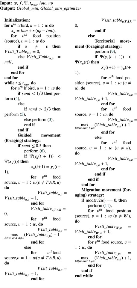
Algorithm 1. Presents the AHA pseudocode.

2.3 Chaos property

Chaos theory studies the nonlinear system dynamics. In chaos-excited systems, a small variation in the initial conditions can generate a highly diverse effect on the system output. Ergodicity, regularity and inherent stochasticity are the chaos properties (Wu and Chen, 1996) which excite a chaotic system to search the entire space in a chaotic way with a high probability of global convergence. Generally, in the population-initialization stage, an optimization algorithm involves the random number sequence generators to initialize the search space. A chaotic optimization process utilizes the non-periodic chaotic sequences in place of the randomly generated sequences (Hossein Gandomi et al., 2013) for a deeper and faster exploitation and a thorough exploration of the space, hence minimizing the local convergence problem.

2.3.1 Chaotic maps

The nonlinear dynamics of chaos energizes the searching behaviour of an optimization algorithm with a more thorough and faster search characteristic, and this is why the various chaotic maps have been effectively applied in solving different real world optimization problems. The performance of these chaotic maps, when integrated with a certain algorithm framework, differs from one another, and each map has a unique initialization functioning range. Choosing the starting point inside the limiting range is a crucial factor for a chaotic map’s performance because it has a significant impact on the final outcome. Table 1 contains a listing of various chaotic maps (Wang et al., 2001; Ahmad Rather and Shanthi Bala, 2020), and for all these maps, we choose a starting point value of 0.7 within the limiting range for initialization from 0 to 1. On the basis of the most robust optimization in a statistical result analysis (Table 1) of 30 individual runs of a performance test of AHA algorithm and each of its 10 chaotic variants, $i.e.$ each combination of AHA framework and each of the listed chaotic maps for the considered PVD optimization problem, the Gauss/mouse (Peitgen et al., 1992; Jothiprakash and Arunkumar, 2013) map has been considered for all the required simulation studies of the present work.

Table 1

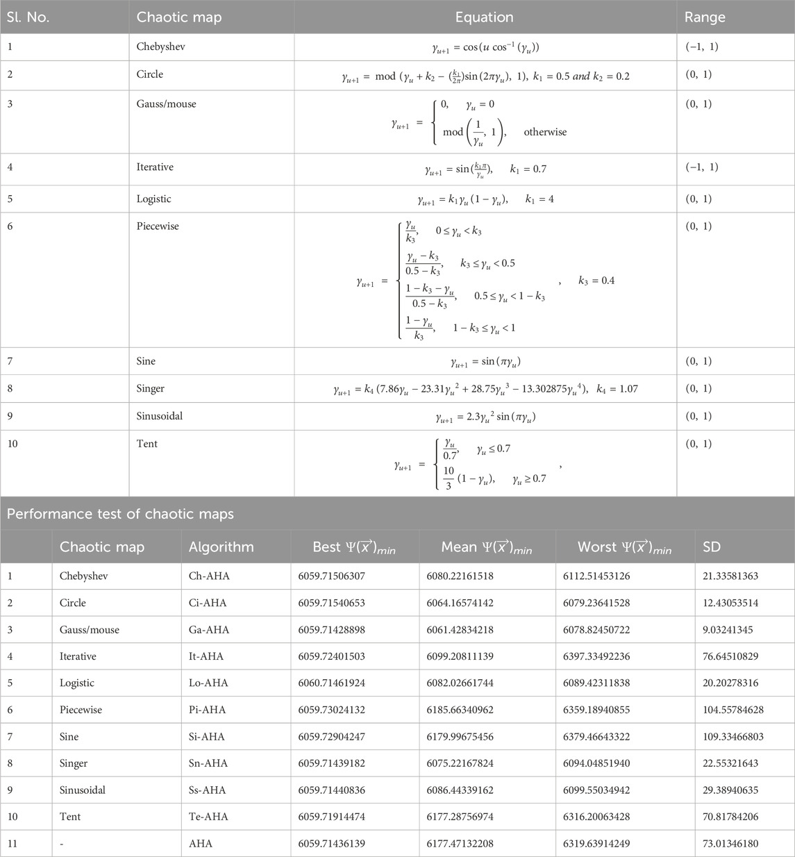
Table 1. Chaotic maps.

2.4 Oppositional chaotic artificial hummingbird algorithm (OCAHA)

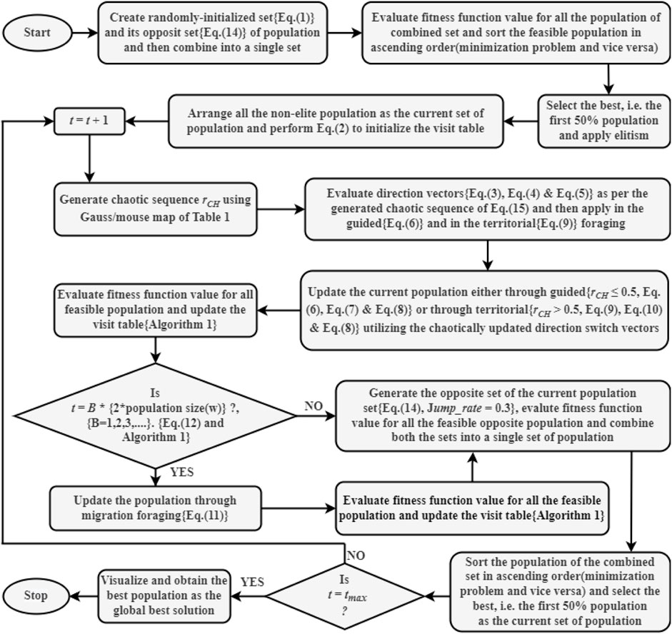
During initialization of the proposed method, an opposite population set is generated using the OBL rule Equation 14, and then it is combined with the randomly initialized set to create a single set of solutions or population. Afterward, the element population of this combined set are sorted in ascending (minimizing objective) or in descending (maximizing objective) orders, and then the first (best) 50$\%$ solutions are selected as the current population to process (update) in the 1st iteration’s events, $i.e$ either through guided ($r_{CH}^{(u)}\le 0.5$) or through territorial $\left(r_{CH}^{(u)}>0.5\right)$ strategies and then through migration strategy (at every $2w$ generations or iterations as defined in Equation 12). Here, the chaotic sequence $r_{CH}^{(u)}$ is generated using the Gauss/mouse map (Table 1) in $(\mathrm{0,1})$ for replacing the randomly generated sequences of the direction-controlling vectors of Equations 3–5 as defined in the Equation 15 to control the three hummingbird flying skills in a more effective manner to ensure a thorough search of the entire space. These chaotically updated direction switch vectors update the search processes of guided Equation 6 and territorial Equation 9 foraging chaotically. The occurrence of these two events is controlled by the specified $r_{CH}^{(u)}$ values of Equation 16 to achieve a more balanced search towards global convergence. After updating through either guided or territorial and the migrating (at every $2w$ generations or iterations as defined in Equation 12) events during each iteration, again the opposition-based learning rule is implemented on the basis of a considered jumping probability ($Jump\text{\_}\mathit{rate}=0.3$) to bring the current solutions or the current population in close vicinity of the desired solution. If the $rand$ is greater than the $Jump\text{\_}\mathit{rate}$, the opposite variable of the corresponding current design variable is determined by Equation 14, otherwise, a current variable and its opposite variable will be same. In this way, each current variable is to be processed to generate the opposite population set, and then both the sets are combined. Afterward, this combined set are sorted according to the objective of optimization problem to select the best (first 50$\%$) solutions of the set as the current population for processing (updating) in the 2nd iteration, and the same updating continues up to the maximum generations to reach the closest to the global solution.

$\begin{array}{c}\hfill {I_u}_{\left(CH\right)}^{\left(i\right)}=\left\{\begin{array}{c}{I_u}^{\left(i\right)}\text{of}\left(3\right),1/3\le r_{CH}^{\left(u\right)}\le 2/3,\left(\text{Axial\hspace{0.17em}flight}\right)\hfill \\ {I_u}^{\left(i\right)}\text{of}\left(4\right),r_{CH}^{\left(u\right)}<1/3,\left(\text{Diagonal\hspace{0.17em}flight}\right)\hfill \\ {I_u}^{\left(i\right)}\text{of}\left(5\right),r_{CH}^{\left(u\right)}>2/3,\left(\text{Omnidirectional\hspace{0.17em}flight}\right),\hfill \end{array}\right.\end{array}(15)$

$i=1,\dots ,f;u=1,\dots ,w$

$\begin{array}{c}\hfill r_{CH}^{\left(u\right)}=\left\{\begin{array}{c}\le 0.5\to \text{Guided\hspace{0.17em}foraging\hspace{0.17em}strategy}\hfill \\ \text{otherwise}\to \text{Territorial\hspace{0.17em}foraging\hspace{0.17em}strategy,}\hfill \end{array}\right.\end{array}(16)$

$u=1,\dots ,w$

Figure 1 presents the algorithmic flowchart of OCAHA.

Figure 1

Figure 1. Flowchart of the OCAHA algorithm.

2.5 OCAHA implementation

The section describes the algorithmic steps for implementing the OCAHA method to optimize all the cases of the study.

Population-initialization:

$◦$ Set population size $w$, stopping criterion (maximum generations) $t_{\mathit{max}}$, optimizing variables and their limits (f, x→, low, up), optimization objective $(\mathrm{\Psi },\mathrm{\Psi }$(x→)) function, and the required constant and constraint criteria for the implementing test case,

$◦$ Generate the randomly-initialized population set by Equation 1 and its opposite set by Equation 14; combine them as a single set; limit the problem variables to their functional range; measure the fitness values using the concerned objective $\left(\mathrm{\Psi }(\stackrel{}{x})\right)$; ensure the constraints fulfilling criteria for all the population and make them feasible; sort the population in ascending order (for objective minimization and vice versa); select the first (best) 50% population; preserve some elite population or elite solutions; find the best (current best) population; and then ready to update these non-elite population (current population) in the $1^{st}$ iteration of the optimization process,

$◦$ Initialize the visit table by Equation 2,

• $1^{st}(\text{t}=1)$ iteration, (either through guided (when $r_{CH}\le 0.5$) or through territorial (when $r_{CH}>0.5$) foraging strategy).

◦ Obtain the chaotic $r_{CH}$ (sequence) values from the Gauss/mouse map (Table 1),

◦ Evaluate the chaotic direction switch vectors (${I_u}_{(CH)}$ of Equation 15) using Equations 3–5,

• Guided foraging strategy $(r_{CH}\le 0.5)$:

◦ Update the current population through this event (Equations 6–8) using the chaotic direction vectors (${I_u}_{(CH)}$ of Equation 15), check the feasibility of the updated population, and then arrange them as the current population set to update in the next event,

◦ Find the current best population, $i.e$ the best of current population set, and then update the visit table’s positions (levels) according to the Algorithm 1 pseudocode,

• End (guided foraging strategy)

• Territorial foraging strategy $(r_{CH}>0.5)$:

◦ Update the current population through this event (Equations 8–10) using the chaotic direction vectors (${I_u}_{(CH)}$ of Equation 15), check the feasibility of the updated population, and then arrange them as the current population set to update in the next event,

◦ Find the current best population, and then update the visit table according to the pseudocode (Algorithm 1),

End (territorial foraging strategy)

• Migration foraging strategy:

◦ Update the current population through the migration foraging event (Equation 11) at every 2$w$ generations or iterations ($G_M$ of Equation 12), check the feasibility of the updated population, and then arrange them as the current population set to update in the next event,

◦ Find the current best population, and then update the visit table according to the pseudocode (Algorithm 1),

• End (migration foraging strategy)

• Opposition-based learning rule, OBL:

◦ Based on the considered jumping ($Jump\text{\_}\mathit{rate}=0.3$) probability, get the opposite set of the current population set using Equation 14 (if the $rand$, $i.e.$ the randomly generated number is greater than 0.3, the corresponding opposite variable is generated by Equation 14, otherwise, a current variable and its opposite variable will be of same value),

◦ Combine both the sets into a single population set, and then check the constraints fulfilling criteria for all these population and make them feasible,

◦ sort the population in ascending order (for objective minimization and vice versa), and then select the first (best) 50% solutions to use as current population for $2^{nd}$ iteration,

◦ Find the current best solution,

• Next iterations$(\text{t}=\text{t}+1)$,

• Visualize and get the global solution.

3 Descriptions and formulations of optimization problems

The section describes the 29 functions of CEC 2017 unconstrained test suite (Awad et al., 2017), and thorough mathematical representations of the ten engineering problems.

3.1 CEC 2017 unconstrained functions

The CEC 2017 test functions (Awad et al., 2017) have been solved to check the local exploitation, avoidance of local optimality, global exploration, solutional accuracy and the other performance measures of OCAHA. These functions are the standard single-objective minimization problems for real-parameter numerical optimization. Table 2 lists the information for these 29 unconstrained standard functions, and their detailed clarification are available in (Awad et al., 2017). Unimodal (F 1-F 3) functions assess the convergence accuracy of a process, the global optimizing potential of a method is tested by simple multimodal (F 4-F 10) and hybrid (F 11-F 20) functions, and the composition (F 21-F 30) functions evaluate the avoidance of the local optima entrapment issue of an optimization algorithm. The Hybrid and the composition functions are more complicated than the unimodal and the simple multimodal functions, and are appropriate for evaluating the optimizing ability of an algorithm in the real-world cases.

Table 2

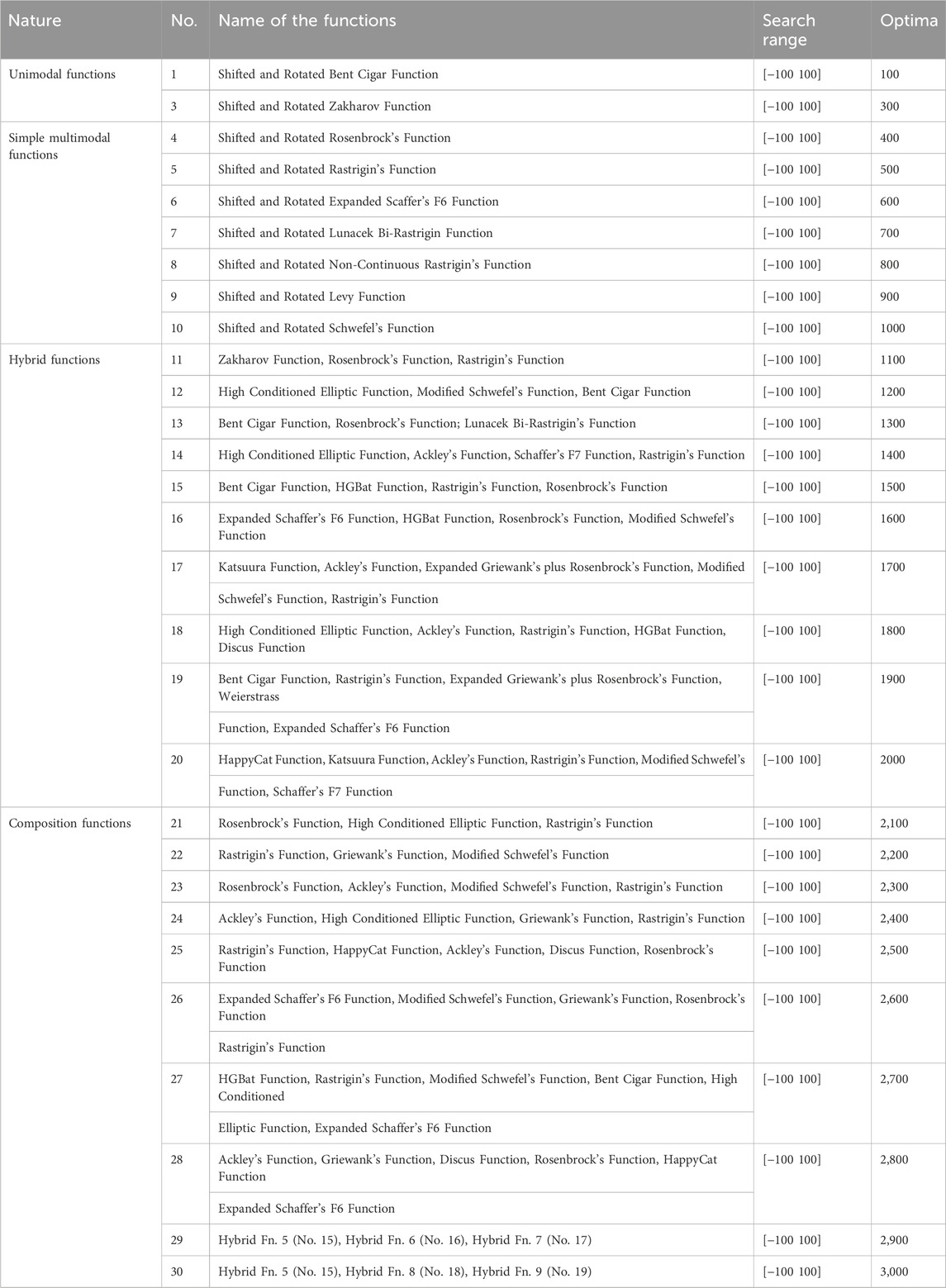
Table 2. CEC 2017 unconstrained functions (Awad et al., 2017).

3.2 Engineering design problems

The detailed descriptions of the ten number considered problems of mechanical engineering design optimization have been presented in this section.

3.2.1 Welded beam design (WBD)

A beam of rectangular cross-section of width $W$ and thickness $T_B$ is to be welded to a rigid frame on either along its four joining sides (defined by $X_1=1$) or on its two longitudinal parallel joining sides (defined by $X_1=0$) to support a constant perpendicular load $F$ at its free end of length $L$. The beam materials (defined by $X_2$) and the types of weld (defined by $X_1$) have been given in Table 3. The weld thickness is $T_W$ and the length of the weld along its longitudinal parallel joining sides is $l$. The overall fabricating cost of this welded cantilever is to be minimized as the single objective (Kennedy and Eberhart, 1997; Datta and Figueira, 2011) of the problem.

$\left.\begin{array}{c}\text{Designing\hspace{0.17em}variables}\left(\text{to\hspace{0.17em}optimize}\right):\hfill \\ \stackrel{}{x\to }=\left[X_1{X}_2{T}_{W}W{T}_{B}l\right]\hfill \\ \text{Objective\hspace{0.17em}function\hspace{0.17em}}\left(\text{to\hspace{0.17em}minimize}\right)\text{:}\hfill \\ \hfill \mathrm{\Psi }(\stackrel{}{x\to })=\left(\left(1+R_1\right)\left(X_{1}W+l\right){T_W}^2+R_{2}W{T}_B\left(L+l\right)\right)\end{array}\right\}(17)$

$\left.\begin{array}{cc}\hfill & \text{The\hspace{0.17em}problem\hspace{0.17em}design\hspace{0.17em}inequality\hspace{0.17em}constraints\hspace{0.17em}to\hspace{0.17em}satisfy:}\hfill \\ \hfill C_{1x}& =\text{Induced\hspace{0.17em}bending\hspace{0.17em}stress\hspace{0.17em}condition\hspace{0.17em}in\hspace{0.17em}the\hspace{0.17em}beam}-\hfill \\ \hfill & =s_x-s_{max}=s_x-\sigma \le 0\hfill \\ \hfill C_{2x}& =\text{Condition\hspace{0.17em}for\hspace{0.17em}critical\hspace{0.17em}buckling\hspace{0.17em}load\hspace{0.17em}in\hspace{0.17em}lateral\hspace{0.17em}direction}\hfill \\ \hfill & =F-F_{cx}\le 0\hfill \\ \hfill C_{3x}& =\text{Maximum\hspace{0.17em}deflection\hspace{0.17em}of\hspace{0.17em}the\hspace{0.17em}beam}={\epsilon }_x-{\epsilon }_{max}\le 0\hfill \\ \hfill C_{4x}& =\text{Maximum\hspace{0.17em}limit\hspace{0.17em}of\hspace{0.17em}generated\hspace{0.17em}shear\hspace{0.17em}stress\hspace{0.17em}in\hspace{0.17em}the\hspace{0.17em}welding}\hfill \\ \hfill & ={\tau }_x-{\tau }_{max}={\tau }_x-0.577\sigma \le 0\hfill \end{array}\right\}(18)$

$\left.\begin{array}{cc}\hfill \text{Desi}& {\mathrm{g}\mathrm{n}\mathrm{i}\mathrm{n}\mathrm{g}\mathrm{v}\mathrm{a}\mathrm{r}\mathrm{i}\mathrm{a}\mathrm{b}\mathrm{l}\mathrm{e}s}^{\prime }\text{intervals:}{X}_1\in \left\{\mathrm{0,1}\right\},X_2\in \left\{\mathrm{0,1,2,3}\right\}\text{and}\hfill \\ T_W\hfill & =\text{Variable}\left(\text{discrete}\right)\text{\hspace{0.17em}in\hspace{0.17em}the\hspace{0.17em}multiples\hspace{0.17em}of\hspace{0.17em}}0.0625=\left[0.0625,2.0\right]inch.\hfill \\ W\hfill & =\text{Variable\hspace{0.17em}}\left(\text{discrete}\right)\text{\hspace{0.17em}in\hspace{0.17em}the\hspace{0.17em}multiples\hspace{0.17em}of\hspace{0.17em}}0.0625=\left[2.0,20.0\right]inch.\hfill \\ T_B\hfill & =\text{Variable}\left(\text{discrete}\right)\text{\hspace{0.17em}in\hspace{0.17em}the\hspace{0.17em}multiples\hspace{0.17em}of\hspace{0.17em}}0.0625=\left[0.0625,2.0\right]inch.\hfill \\ l\hfill & =\text{Variable}\left(\text{continuous}\right)=\left[1.0,10.0\right]inch.\hfill \end{array}\right\}(19)$

$\left.\begin{array}{cc}\hfill & \text{Constant\hspace{0.17em}inputs\hspace{0.17em}for\hspace{0.17em}the\hspace{0.17em}problem:}\hfill \\ \hfill s_{\mathit{max}}& =\text{Maximum\hspace{0.17em}limit\hspace{0.17em}of\hspace{0.17em}bending\hspace{0.17em}stress}=\sigma =\mathrm{30,000}psi\hfill \\ \hfill {\tau }_{\mathit{max}}& =\text{Maximum\hspace{0.17em}limit\hspace{0.17em}of\hspace{0.17em}shear\hspace{0.17em}stress}=0.577\sigma \hfill \\ \hfill {\epsilon }_{\mathit{max}}& =\text{Maximum\hspace{0.17em}limit\hspace{0.17em}of\hspace{0.17em}deflection}=0.25inch.\hfill \\ \hfill E\hfill & =\text{Modulus\hspace{0.17em}of\hspace{0.17em}elasticity\hspace{0.17em}of\hspace{0.17em}beam\hspace{0.17em}material}=30\times 10^{6}psi\hfill \\ \hfill G\hfill & =\text{Modulus\hspace{0.17em}of\hspace{0.17em}rigidity\hspace{0.17em}of\hspace{0.17em}beam\hspace{0.17em}material}=12\times 10^{6}psi\hfill \\ \hfill L\hfill & =\text{Hanging\hspace{0.17em}length\hspace{0.17em}of\hspace{0.17em}the\hspace{0.17em}beam\hspace{0.17em}from\hspace{0.17em}its\hspace{0.17em}rigid\hspace{0.17em}support\hspace{0.17em}end}=14inch.\hfill \\ \hfill F\hfill & =\text{Constant\hspace{0.17em}perpendicular\hspace{0.17em}load\hspace{0.17em}concentrated\hspace{0.17em}at\hspace{0.17em}the\hspace{0.17em}free\hspace{0.17em}end\hspace{0.17em}of\hspace{0.17em}the\hspace{0.17em}beam}\hfill \\ \hfill & =6000lb\hfill \end{array}\right\}(20)$

$\left.\begin{array}{c}\text{Input\hspace{0.17em}relations\hspace{0.17em}for\hspace{0.17em}the\hspace{0.17em}problem:}\hfill \\ {\sigma }_x=\text{Induced\hspace{0.17em}bending\hspace{0.17em}stress\hspace{0.17em}in\hspace{0.17em}the\hspace{0.17em}beam}=\frac{6FL}{T_B{W}^2}\hfill \\ {\tau }_p=\text{primary\hspace{0.17em}shear\hspace{0.17em}stress\hspace{0.17em}developed\hspace{0.17em}in\hspace{0.17em}the\hspace{0.17em}weld}=\frac{F}{\sqrt{2}{T}_{W}l}\text{for}{X}_1=0,\hfill \\ \hfill =\frac{F}{\sqrt{2}{T}_W\left(l+W\right)}\text{for}{X}_1=1\\ M_B=\text{Bending\hspace{0.17em}moment\hspace{0.17em}developed\hspace{0.17em}at\hspace{0.17em}the\hspace{0.17em}support\hspace{0.17em}end}=F\left(L+0.5l\right)\hfill \\ {\rho }_W=\text{Torsional\hspace{0.17em}radius\hspace{0.17em}of\hspace{0.17em}the\hspace{0.17em}weld}=\sqrt{{\left(\frac{l}{2}\right)}^2+{\left(\frac{W+T_W}{2}\right)}^2}\text{for}{X}_1=0,\hfill \\ \hfill =max\left\{\sqrt{{\left(\frac{l}{2}\right)}^2+{\left(\frac{W+T_W}{2}\right)}^2},\sqrt{{\left(\frac{W}{2}\right)}^2+{\left(\frac{l+T_W}{2}\right)}^2}\right\}\text{for}{X}_1=1\\ J_W=\text{Polar\hspace{0.17em}moment\hspace{0.17em}of\hspace{0.17em}inertia\hspace{0.17em}of\hspace{0.17em}the\hspace{0.17em}weld}=\sqrt{2}{T}_{W}l\left\{\frac{l^2}{12}+\frac{{\left(T_W+W\right)}^2}{4}\right\}\text{for}{X}_1=0,\hfill \\ \hfill =\left[\sqrt{2}{T}_{W}l\left\{\frac{l^2}{12}+\frac{{\left(T_W+W\right)}^2}{4}\right\}+\sqrt{2}{T}_{W}W\left\{\frac{W^2}{12}+\frac{{\left(T_W+l\right)}^2}{4}\right\}\right]\text{for}{X}_1=1\\ Cos\gamma =\frac{\frac{l}{2}}{{\rho }_W}\text{for}{X}_1=0,\hfill \\ \hfill =\frac{\frac{l}{2}}{{\rho }_W}\text{if}l<W,\text{for}{X}_1=1,\\ \hfill =\frac{\frac{W}{2}}{{\rho }_W}\text{otherwise,}\text{for}{X}_1=1\\ {\tau }_s=\text{Secondary\hspace{0.17em}shear\hspace{0.17em}stress\hspace{0.17em}developed\hspace{0.17em}in\hspace{0.17em}the\hspace{0.17em}weld}=\frac{M_B{\rho }_W}{J_W}\hfill \\ {\tau }_R\text{or}{\tau }_x=\text{Resultant\hspace{0.17em}shear\hspace{0.17em}stress\hspace{0.17em}in\hspace{0.17em}the\hspace{0.17em}weld}=\sqrt{{\tau }_p^2+{\tau }_s^2+2{\tau }_p{\tau }_{s}Cos\gamma }\hfill \\ {\epsilon }_x=\text{Axial\hspace{0.17em}deflection\hspace{0.17em}of\hspace{0.17em}the\hspace{0.17em}beam}=\frac{4F{L}^3}{E{T}_B{W}^3}\hfill \\ F_{cx}={\text{Beam}}^{\prime }\text{s\hspace{0.17em}critical\hspace{0.17em}load\hspace{0.17em}for\hspace{0.17em}lateral\hspace{0.17em}buckling\hspace{0.17em}with\hspace{0.17em}respect\hspace{0.17em}to\hspace{0.17em}an\hspace{0.17em}axis\hspace{0.17em}parallel}-\hfill \\ \hfill {\text{to\hspace{0.17em}it}}^{\prime }\text{s\hspace{0.17em}width,\hspace{0.17em}W}=\frac{4.013W{T_B}^3}{6L^2}\sqrt{EG}\left(1-\frac{W}{4L}\sqrt{\frac{E}{G}}\right)\end{array}\right\}(21)$

Table 3

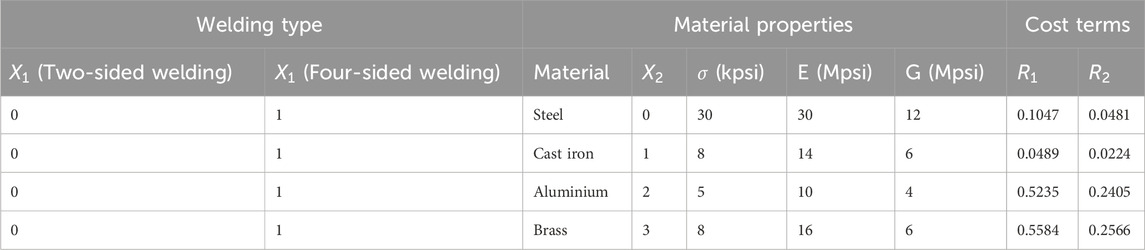
Table 3. Welding types, material properties and cost term values of WBD problem.

3.2.2 Belt-pulley drive design (BPDD)

The objective of the belt-pulley drive problem (Venkata Rao and Pawar, 2020; Thamaraikannan and Thirunavukkarasu, 2014) is to minimize the pulleys’ total weight in a flat belt-pulley drive system (Figure 2 for BPDD). From the driver pulley of diameter $d_{DR}$, the required power of 10 $hp$ is to be transmitted to the common shaft mounting the $3^{\text{rd}}$ and the $4^{\text{th}}$ pulley of diameters ${d_{DR}}^{\prime }$ and ${d_{DN}}^{\prime }$ respectively, and then through this $4^{\text{th}}$ pulley to the output shaft mounting the driven pulley $\left(d_{DN}\right)$. The driver pulley diameter $d_{DR}$, driven pulley diameter $d_{DN}$ and the width of the pulleys $B$ are the three continuous designing variables along with a tensile stress constraint for flat belt and a dimensional constraint on the pulleys’ width have been considered to minimize the pulleys’ total weight to avoid any shaft and bearing failures.

$\left.\begin{array}{c}\text{Designing\hspace{0.17em}variables}\left(\text{to\hspace{0.17em}optimize}\right):\hfill \\ \stackrel{}{x\to }=\left[d_{DR}{d}_{DN}B\right]\hfill \\ \text{Objective\hspace{0.17em}function\hspace{0.17em}}\left(\text{to\hspace{0.17em}minimize}\right)\text{:}\hfill \\ \mathrm{\Psi }(\stackrel{}{x\to })=\left(\pi {\rho }_{P}B\left(d_{DR}{T}_{DR}+d_{DN}{T}_{DN}+{d_{DR}}^{\prime }{T_{DR}}^{\prime }+{d_{DN}}^{\prime }{T_{DN}}^{\prime }\right)\right)kg\hfill \end{array}\right\}(22)$

$\left.\begin{array}{cc}\hfill \text{The}& \text{problem\hspace{0.17em}design\hspace{0.17em}inequality\hspace{0.17em}constraints\hspace{0.17em}to\hspace{0.17em}satisfy:}\hfill \\ \hfill C_{1x}& =\text{Induced\hspace{0.17em}tensile\hspace{0.17em}stress\hspace{0.17em}condition\hspace{0.17em}in\hspace{0.17em}the\hspace{0.17em}flat}-\text{belt}\hfill \\ \hfill & =S_B-\frac{F_T}{B{T}_B}=B{d}_{DN}-381.97\ge 0\hfill \\ \hfill C_{2x}& =\text{Condition\hspace{0.17em}on\hspace{0.17em}the\hspace{0.17em}width\hspace{0.17em}of\hspace{0.17em}the\hspace{0.17em}pulleys}\hfill \\ \hfill & =0.25d_{DR}-B=d_{DR}-4B\ge 0\hfill \end{array}\right\}(23)$

$\left.\begin{array}{cc}\text{Specified}\hfill & \text{intervals\hspace{0.17em}of\hspace{0.17em}designing\hspace{0.17em}variables:}\hfill \\ \hfill d_{DR}& =\text{Continuous\hspace{0.17em}variable}=\left[\mathrm{15,25}\right]cm\hfill \\ \hfill d_{DN}& =\text{Continuous\hspace{0.17em}variable}=\left[\mathrm{70,80}\right]cm\hfill \\ \hfill B& =\text{Continuous\hspace{0.17em}variable}=\left[\mathrm{4,10}\right]cm\hfill \end{array}\right\}(24)$

$\left.\begin{array}{c}\text{Constant}\text{inputs\hspace{0.17em}for\hspace{0.17em}the\hspace{0.17em}problem:}\hfill \\ R_{DR}=\text{RPM\hspace{0.17em}of\hspace{0.17em}the}{1}^{\text{st}}i.e.\text{the\hspace{0.17em}driver\hspace{0.17em}pulley}=1000rpm\hfill \\ R_{DN}=\text{RPM\hspace{0.17em}of\hspace{0.17em}the}{2}^{\text{nd}}i.e.\text{the\hspace{0.17em}driven\hspace{0.17em}pulley}=250rpm\hfill \\ {R_{DR}}^{\prime }=\text{RPM\hspace{0.17em}of\hspace{0.17em}the}{3}^{\text{rd}}\text{pulley}=500rpm\hfill \\ {R_{DN}}^{\prime }=\text{RPM\hspace{0.17em}of\hspace{0.17em}the}{4}^{\text{th}}\text{pulley}=500rpm\hfill \\ T_B={\text{Flat\hspace{0.17em}belt}}^{\prime }\text{s\hspace{0.17em}thickness}=1cm\hfill \\ S_B=\text{Maximum\hspace{0.17em}tensile\hspace{0.17em}stress\hspace{0.17em}limit\hspace{0.17em}in\hspace{0.17em}the\hspace{0.17em}flat}-\text{belt}=30kg{cm}^{-2}\hfill \\ {\rho }_P=\text{Mass\hspace{0.17em}density\hspace{0.17em}of\hspace{0.17em}the\hspace{0.17em}material\hspace{0.17em}of\hspace{0.17em}the\hspace{0.17em}pulleys}=7.2\times 10^{-3}kgc{m}^{-3}\hfill \\ F_T={\text{Flat}-\text{belt}}^{\prime }\text{s\hspace{0.17em}tension\hspace{0.17em}in\hspace{0.17em}the\hspace{0.17em}tight}-\text{side}=\text{in}kgf\hfill \\ F_S={\text{Flat}-\text{belt}}^{\prime }\text{s\hspace{0.17em}tension\hspace{0.17em}in\hspace{0.17em}the\hspace{0.17em}slack}-\text{side}=\text{in}kgf\hfill \\ P_{BP}=\text{Power\hspace{0.17em}to\hspace{0.17em}be\hspace{0.17em}transmitted}=10hp=10\times 75kgm{s}^{-1}\hfill \end{array}\right\}(25)$

$\left.\begin{array}{cc}\hfill & \text{Input\hspace{0.17em}relations\hspace{0.17em}for\hspace{0.17em}the\hspace{0.17em}problem:}\hfill \\ \hfill T_{DR}& =\text{Thickness\hspace{0.17em}of\hspace{0.17em}the}{1}^{\text{st}}\text{or\hspace{0.17em}driver\hspace{0.17em}pulley}=0.1\times d_{DR}cm\hfill \\ \hfill T_{DN}& =\text{Thickness\hspace{0.17em}of\hspace{0.17em}the\hspace{0.17em}}{2}^{\text{nd}}\text{or\hspace{0.17em}driver\hspace{0.17em}pulley}=0.1\times d_{DN}cm\hfill \\ \hfill {T_{DR}}^{\prime }& =\text{Thickness\hspace{0.17em}of\hspace{0.17em}the\hspace{0.17em}}{3}^{\text{rd}}\text{pulley}=0.1\times {d_{DR}}^{\prime }cm\hfill \\ \hfill {T_{DN}}^{\prime }& =\text{Thickness\hspace{0.17em}of\hspace{0.17em}the\hspace{0.17em}}{4}^{\text{th}}\text{pulley}=0.1\times {d_{DN}}^{\prime }cm\hfill \\ \hfill V_{DR}& =\text{Tangential\hspace{0.17em}velocity\hspace{0.17em}of\hspace{0.17em}the\hspace{0.17em}}{1}^{\text{st}}\text{or\hspace{0.17em}driver\hspace{0.17em}pulley}=\pi d_{DR}{R}_{DR}cm{min}^{-1}\hfill \\ \hfill {V_{DR}}^{\prime }& =\text{Tangential\hspace{0.17em}velocity\hspace{0.17em}of\hspace{0.17em}the\hspace{0.17em}}{3}^{\text{rd}}\text{pulley}=\pi {d_{DR}}^{\prime }{R_{DR}}^{\prime }cm{min}^{-1}\hfill \\ \hfill & \pi d_{DR}{R}_{DR}=\pi {d_{DR}}^{\prime }{R_{DR}}^{\prime }\Rightarrow {d_{DR}}^{\prime }=2d_{DR}\hfill \\ \hfill V_{DN}& =\text{Tangential\hspace{0.17em}velocity\hspace{0.17em}of\hspace{0.17em}the\hspace{0.17em}}{2}^{\text{nd}}\text{or\hspace{0.17em}driver\hspace{0.17em}pulley}=\pi d_{DN}{R}_{DN}cm{min}^{-1}\hfill \\ \hfill {V_{DN}}^{\prime }& =\text{Tangential\hspace{0.17em}velocity\hspace{0.17em}of\hspace{0.17em}the\hspace{0.17em}}{4}^{\text{th}}\text{pulley}=\pi {d_{DN}}^{\prime }{R_{DN}}^{\prime }cm{min}^{-1}\hfill \\ \hfill & \pi d_{DN}{R}_{DN}=\pi {d_{DN}}^{\prime }{R_{DN}}^{\prime }\Rightarrow {d_{DN}}^{\prime }=0.5d_{DN}\hfill \\ \hfill \frac{F_S}{F_T}& =\text{Tension}\left(\text{slack\hspace{0.17em}side\hspace{0.17em}to\hspace{0.17em}tight\hspace{0.17em}side}\right)\text{\hspace{0.17em}ratio\hspace{0.17em}of\hspace{0.17em}the\hspace{0.17em}flat}-\text{belt}=0.5\hfill \\ \hfill P_{BP}& =\text{Power\hspace{0.17em}to\hspace{0.17em}be\hspace{0.17em}transmitted\hspace{0.17em}by\hspace{0.17em}the\hspace{0.17em}belt}-\text{pulley\hspace{0.17em}drive\hspace{0.17em}system}=\left(F_T-F_S\right)\frac{\left(\pi d_{DN}{R}_{DN}\right)}{6000}\hfill \\ \hfill & \left(F_T-F_S\right)\frac{\left(\pi d_{DN}{R}_{DN}\right)}{6000}=10\times 75kgm{s}^{-1}\Rightarrow F_T=\frac{2864789}{d_{DN}{R}_{DN}}kgf\hfill \end{array}\right\}(26)$

Figure 2

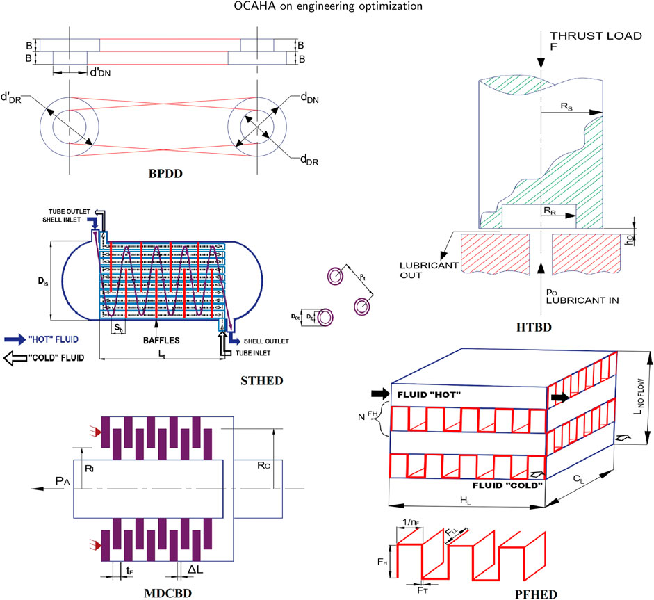
Figure 2. Schematic diagram for BPDD, HTBD, PFHED, STHED and MDCBD problems.

3.2.3 Helical compression spring design (HCSD)

This problem (Datta and Figueira, 2011; Sandgren, 1990) deals with the minimization of the wire volume, $i.e$ the weight of a coil spring (helical compression) of its winding coil’s outside diameter $D_O$, wire diameter $d_W$ and the spring coils number $N$. The spring must sustain a steady axial compressive load $F_{\mathit{max}}$ without failing.

$\left.\begin{array}{c}\text{Designing}\text{variables}\left(\text{to\hspace{0.17em}optimize}\right):\hfill \\ \stackrel{}{x\to }=\left[D_O{d}_{W}N\right]\hfill \\ \text{Objective}\text{function}\left(\text{to\hspace{0.17em}minimize}\right):\hfill \\ \mathrm{\Psi }(\stackrel{}{x\to })=\left(\frac{{\pi }^2}{4}{d_W}^2{D}_O\left(N+2\right)\right){inch}^3\hfill \end{array}\right\}(27)$

$\left.\begin{array}{cc}\hfill \text{The}& \text{problem\hspace{0.17em}design\hspace{0.17em}inequality\hspace{0.17em}constraints\hspace{0.17em}to\hspace{0.17em}satisfy:}\hfill \\ \hfill C_{1x}& =\text{condition\hspace{0.17em}of\hspace{0.17em}Maximum\hspace{0.17em}shear\hspace{0.17em}stress\hspace{0.17em}induced\hspace{0.17em}in\hspace{0.17em}the\hspace{0.17em}spring}={\tau }_{\mathit{max}}-\frac{8S_F{F}_{\mathit{max}}{D}_O}{\pi {d_W}^3}\ge 0\hfill \\ \hfill C_{2x}& =\text{Maximum\hspace{0.17em}free\hspace{0.17em}length\hspace{0.17em}of\hspace{0.17em}the\hspace{0.17em}spring}={\left(L_F\right)}_{\mathit{max}}-L_F\hfill \\ \hfill & ={\left(L_F\right)}_{\mathit{max}}-\epsilon -1.05\left(N+2\right)d_W\ge 0\hfill \\ \hfill C_{3x}& =\text{Minimum\hspace{0.17em}wire\hspace{0.17em}diameter\hspace{0.17em}condition}=d_W-{d_W}_{\mathit{min}}\ge 0\hfill \\ \hfill C_{4x}& =\text{Condition\hspace{0.17em}of\hspace{0.17em}maximum\hspace{0.17em}mean\hspace{0.17em}diameter\hspace{0.17em}of\hspace{0.17em}winding\hspace{0.17em}coil}={D_O}_{\mathit{max}}-D_O-d_W\ge 0\hfill \\ \hfill C_{5x}& ={\text{Coil}}^{\prime }\text{s\hspace{0.17em}mean\hspace{0.17em}winding\hspace{0.17em}diameter\hspace{0.17em}to\hspace{0.17em}wire\hspace{0.17em}diameter\hspace{0.17em}ratio}=\frac{D_O-d_W}{d_W}-3\ge 0\hfill \\ \hfill C_{6x}& ={\text{The\hspace{0.17em}spring}}^{\prime }\text{s\hspace{0.17em}maximum\hspace{0.17em}permitted\hspace{0.17em}preload\hspace{0.17em}deflection}={\epsilon }_{Pmax}-{\epsilon }_P\ge 0\hfill \\ \hfill C_{7x}& =\text{Spring\hspace{0.17em}free\hspace{0.17em}length\hspace{0.17em}criterion\hspace{0.17em}in\hspace{0.17em}the\hspace{0.17em}preloaded\hspace{0.17em}condition}\hfill \\ \hfill & =L_F-{\epsilon }_P-\left(\frac{F_{\mathit{max}}-F_P}{S}\right)-1.05\left(N+2\right)d_W\ge 0\hfill \\ \hfill C_{8x}& =\text{Condition\hspace{0.17em}on\hspace{0.17em}the\hspace{0.17em}deflection\hspace{0.17em}between\hspace{0.17em}preloaded\hspace{0.17em}and\hspace{0.17em}}-\hfill \\ \hfill & -\text{maximum\hspace{0.17em}working\hspace{0.17em}load\hspace{0.17em}postions}=\left(\frac{F_{\mathit{max}}-F_P}{S}\right)-{\epsilon }_M\ge 0\hfill \end{array}\right\}(28)$

$\left.\begin{array}{cc}\hfill \text{Sp}& \text{ecified\hspace{0.17em}intervals\hspace{0.17em}of\hspace{0.17em}designing\hspace{0.17em}variables:}\hfill \\ \hfill D_O& =\text{Variable}\left(\text{continuous}\right)=\left[0.6,3.0\right]inch.\hfill \\ \hfill d_W& =\text{Variable}\left(\text{discrete}\right)=\left[0.2,1.0\right]=\left[0.207,0.225,0.244,0.263-\right.\hfill \\ \hfill & \left.0.283,0.307,0.331,0.362,0.394,0.4375,0.500\right]inch.\hfill \\ \hfill N& =\text{Integer\hspace{0.17em}variable}=\left[\mathrm{1,70}\right]\hfill \end{array}\right\}(29)$

$\left.\begin{array}{cc}\hfill \text{Constant}& \text{inputs\hspace{0.17em}for\hspace{0.17em}the\hspace{0.17em}problem:}\hfill \\ \hfill F_{\mathit{max}}& =\text{Working\hspace{0.17em}load}\left(\text{maximum}\right)=1000lb\hfill \\ \hfill F_P& =\text{Compressive\hspace{0.17em}preload\hspace{0.17em}force}=300lb\hfill \\ \hfill {\tau }_{\mathit{max}}& =\text{Allowable\hspace{0.17em}maximum\hspace{0.17em}shear\hspace{0.17em}stress}=189\times 10^{3}psi\hfill \\ \hfill E& ={\text{Spring\hspace{0.17em}material}}^{\prime }{\text{s\hspace{0.17em}Young}}^{\prime }\text{s\hspace{0.17em}modulus}=30\times 10^{6}psi\hfill \\ \hfill G& ={\text{Spring\hspace{0.17em}material}}^{\prime }\text{s\hspace{0.17em}shear\hspace{0.17em}modulus}=11.5\times 10^{6}psi\hfill \\ \hfill {\left(L_F\right)}_{\mathit{max}}& =\text{Maximum\hspace{0.17em}free\hspace{0.17em}length\hspace{0.17em}of\hspace{0.17em}the\hspace{0.17em}spring}=14inch.\hfill \\ \hfill {d_W}_{\mathit{min}}& =\text{Minimum\hspace{0.17em}wire\hspace{0.17em}diameter\hspace{0.17em}of\hspace{0.17em}the\hspace{0.17em}spring}=0.2inch.\hfill \\ \hfill {D_O}_{\mathit{max}}& ={\text{Spring}}^{\prime }\text{s\hspace{0.17em}winding\hspace{0.17em}coil\hspace{0.17em}maximum\hspace{0.17em}outside\hspace{0.17em}diameter}=3inch.\hfill \\ \hfill {\epsilon }_{Pmax}& =\text{Allowable\hspace{0.17em}maximum\hspace{0.17em}preloaded\hspace{0.17em}deflection\hspace{0.17em}of\hspace{0.17em}the\hspace{0.17em}spring}=6inch.\hfill \\ \hfill {\epsilon }_M& =\text{Deflection\hspace{0.17em}measured\hspace{0.17em}between\hspace{0.17em}preloaded\hspace{0.17em}and\hspace{0.17em}maximum\hspace{0.17em}working}\hfill \\ \hfill & \text{-load\hspace{0.17em}positions}=1.25inch.\hfill \end{array}\right\}(30)$

$\left.\begin{array}{cc}\hfill \text{In}& \text{put\hspace{0.17em}relations\hspace{0.17em}for\hspace{0.17em}the\hspace{0.17em}problem:}\hfill \\ \hfill \epsilon & =\text{Deflection\hspace{0.17em}at\hspace{0.17em}maximum\hspace{0.17em}working\hspace{0.17em}load\hspace{0.17em}position}=\frac{8F_{\mathit{max}}{D_O}^{3}N}{G{d_W}^4}\hfill \\ \hfill S& =\text{Spring\hspace{0.17em}rate\hspace{0.17em}of\hspace{0.17em}deflection}=\frac{G{d_W}^4}{8N{D_O}^3}\hfill \\ \hfill {\epsilon }_P& =\text{Deflection\hspace{0.17em}at\hspace{0.17em}preloaded\hspace{0.17em}position}=\frac{F_P}{S}\hfill \\ \hfill I& =\text{Spring\hspace{0.17em}index}=\frac{D_O}{d_W}\hfill \\ \hfill S_F& =\text{Wahl\hspace{0.17em}stress\hspace{0.17em}factor}=\frac{4I-1}{4I-4}+\frac{0.615}{I}\hfill \end{array}\right\}(31)$

3.2.4 Hydrostatic thrust bearing design (HTBD)

The HTBD (Venkata Rao and Pawar, 2020; Zhao et al., 2022; Siddall, 1982; He et al., 2004; Deb, 1997) case deals with the power loss minimization during the operation of a hydrostatic thrust bearing (Figure 2 for HTBD) requiring a load bearing capacity of $F$, $i.e$ the bearing has to support an axial thrust load $F$. Bearing step radius $R_S$, its recess radius $R_R$, rate of fluid (oil) flow $Q_O$ and the fluid viscosity ${\mu }_O$ are the four designing variables along with seven (constraints) nonlinear inequalities have to be considered for optimizing this problem.

$\left.\begin{array}{c}\text{Designing}\text{variables}\left(\text{to\hspace{0.17em}optimize}\right):\hfill \\ \stackrel{}{x\to }=\left[R_S{R}_R{Q}_O{\mu }_O\right]\hfill \\ \text{Objective}\text{function}\left(\text{to\hspace{0.17em}minimize}\right):\hfill \\ \mathrm{\Psi }(\stackrel{}{x\to })=\left(\frac{\frac{Q_O{p}_O}{0.7}+P_F}{12}\right)ftlb{s}^{-1}\hfill \end{array}\right\}(32)$

$\left.\begin{array}{cc}\hfill \text{The}& \text{problem\hspace{0.17em}design\hspace{0.17em}inequality\hspace{0.17em}constraints\hspace{0.17em}to\hspace{0.17em}satisfy:}\hfill \\ \hfill C_{1x}& ={\text{Bearing\hspace{0.17em}load\hspace{0.17em}carrying\hspace{0.17em}capacity\hspace{0.17em}is\hspace{0.17em}to\hspace{0.17em}be\hspace{0.17em}at\hspace{0.17em}least\hspace{0.17em}equal\hspace{0.17em}to\hspace{0.17em}the\hspace{0.17em}generator}}^{\prime }\text{s\hspace{0.17em}weight}=F-W_G\ge 0\hfill \\ \hfill C_{2x}& =\text{Oil\hspace{0.17em}supply\hspace{0.17em}pressure\hspace{0.17em}at\hspace{0.17em}the\hspace{0.17em}inlet\hspace{0.17em}should,\hspace{0.17em}at\hspace{0.17em}most,\hspace{0.17em}equal\hspace{0.17em}the\hspace{0.17em}maximum\hspace{0.17em}pressure}=p_M-p_O\ge 0\hfill \\ \hfill C_{3x}& =\text{Maximum\hspace{0.17em}permissible\hspace{0.17em}limit\hspace{0.17em}of\hspace{0.17em}Oil\hspace{0.17em}temperature\hspace{0.17em}rise}={\mathrm{\Delta }T}_{O_M}-{\mathrm{\Delta }T}_O\ge 0\hfill \\ \hfill C_{4x}& =\text{Condition\hspace{0.17em}for\hspace{0.17em}minimum\hspace{0.17em}fluid\hspace{0.17em}or\hspace{0.17em}oil\hspace{0.17em}film\hspace{0.17em}thickness}=h_O-h_{\mathit{MIN}}\ge 0\hfill \\ \hfill C_{5x}& =\text{Maximum\hspace{0.17em}permissible\hspace{0.17em}limit\hspace{0.17em}of\hspace{0.17em}recess\hspace{0.17em}diameter}=R_S-R_R\ge 0\hfill \\ \hfill C_{6x}& =\text{Flow\hspace{0.17em}of\hspace{0.17em}fluid\hspace{0.17em}or\hspace{0.17em}oil\hspace{0.17em}is\hspace{0.17em}should\hspace{0.17em}be\hspace{0.17em}laminar\hspace{0.17em}and\hspace{0.17em}the\hspace{0.17em}exit\hspace{0.17em}\&\hspace{0.17em}entrance\hspace{0.17em}loss\hspace{0.17em}of\hspace{0.17em}pressure\hspace{0.17em}must\hspace{0.17em}be\hspace{0.17em}within}-\hfill \\ \hfill & \text{the\hspace{0.17em}}0.1\text{\%\hspace{0.17em}of\hspace{0.17em}the\hspace{0.17em}total\hspace{0.17em}pressure\hspace{0.17em}drop\hspace{0.17em}or\hspace{0.17em}pressure\hspace{0.17em}loss}=0.001-\frac{{\gamma }_O}{g{p}_O}{\left(\frac{Q_O}{2\pi R_S{h}_O}\right)}^2\ge 0\hfill \\ \hfill C_{7x}& =\text{Assumed\hspace{0.17em}average\hspace{0.17em}pressure\hspace{0.17em}limit\hspace{0.17em}to\hspace{0.17em}avoid\hspace{0.17em}surface\hspace{0.17em}damage}[75]=5000-\frac{F}{\pi \left({R_S}^2-{R_R}^2\right)}\ge 0\hfill \end{array}\right\}(33)$

$\left.\begin{array}{cc}\hfill \text{Specified\hspace{0.17em}intervals}& \text{of\hspace{0.17em}designing\hspace{0.17em}variables}\left(\text{all\hspace{0.17em}are\hspace{0.17em}continuous\hspace{0.17em}variables}\right):\hfill \\ \hfill R_S& =\left[\mathrm{1,16}\right]inch,R_R=\left[\mathrm{1,16}\right]inch,\hfill \\ \hfill Q_O& =\left[\mathrm{1,16}\right]inc{h}^3{s}^{-1},{\mu }_O\left(10^{-6}\right)=\left[\mathrm{1,16}\right]lbs{inch}^{-2}\hfill \end{array}\right\}(34)$

$\left.\begin{array}{cc}\hfill \text{Constant}& \text{inputs\hspace{0.17em}for\hspace{0.17em}the\hspace{0.17em}problem:}\hfill \\ \hfill {\gamma }_O& =\text{Specific\hspace{0.17em}weight\hspace{0.17em}of\hspace{0.17em}the\hspace{0.17em}oil})=0.0307lbinc{h}^{-3}\hfill \\ \hfill S_O& =\text{Specific\hspace{0.17em}heat\hspace{0.17em}of\hspace{0.17em}the\hspace{0.17em}oil}=0.5BTUl{b}^{-1}{{}^{◦}F}^{-1}\hfill \\ \hfill C_{1O}& =\text{Constant\hspace{0.17em}for\hspace{0.17em}fluid\hspace{0.17em}or\hspace{0.17em}oil\hspace{0.17em}of\hspace{0.17em}SAE\hspace{0.17em}}20\text{\hspace{0.17em}grade}=10.04\hfill \\ \hfill n_O& =\text{Constant\hspace{0.17em}for\hspace{0.17em}fluid\hspace{0.17em}or\hspace{0.17em}oil\hspace{0.17em}of\hspace{0.17em}SAE\hspace{0.17em}}20\text{\hspace{0.17em}grade}=-3.55\hfill \\ \hfill W_G& =\text{The\hspace{0.17em}generator\hspace{0.17em}Weight}=101000lb\hfill \\ \hfill p_M& =\text{Maximum\hspace{0.17em}allowable\hspace{0.17em}pressure}=1000lb{inch}^{-2}\hfill \\ \hfill {\mathrm{\Delta }T}_{O_M}& =\text{Permissible\hspace{0.17em}limit\hspace{0.17em}for\hspace{0.17em}temperature\hspace{0.17em}rise\hspace{0.17em}of\hspace{0.17em}the\hspace{0.17em}oil}=50{}^{◦}F\hfill \\ \hfill h_{\mathit{MIN}}& =\text{Specified\hspace{0.17em}minimum\hspace{0.17em}oil\hspace{0.17em}or\hspace{0.17em}fluid\hspace{0.17em}film\hspace{0.17em}thickness}=0.001inch\hfill \\ \hfill g& =\text{Acceleration\hspace{0.17em}due\hspace{0.17em}to\hspace{0.17em}gravity}=386.4inch{s}^{-2}\hfill \\ \hfill N& ={\text{Shaft}}^{\prime }\text{s\hspace{0.17em}RPM}=750rpm\hfill \\ \hfill {\eta }_O& =\text{Efficiency\hspace{0.17em}of\hspace{0.17em}oil\hspace{0.17em}or\hspace{0.17em}fluid\hspace{0.17em}pump}=0.7\hfill \\ \hfill J& =\text{Joulean\hspace{0.17em}heat\hspace{0.17em}equivalent}=778\times 12=9336inchlbf{BTU}^{-1}\hfill \end{array}\right\}(35)$

$\left.\begin{array}{cc}\hfill \text{Input}& \text{relations\hspace{0.17em}for\hspace{0.17em}the\hspace{0.17em}problem:}\hfill \\ \hfill p_O& =\text{Inlet\hspace{0.17em}supply\hspace{0.17em}pressure\hspace{0.17em}of\hspace{0.17em}oil}=\frac{6{\mu }_O{Q}_O}{\pi {h_O}^3}{\log }_e\left(\frac{R_S}{R_R}\right)psiorlb{inch}^{-2}\hfill \\ \hfill F& =\text{Load\hspace{0.17em}carrying\hspace{0.17em}capacity\hspace{0.17em}of\hspace{0.17em}the\hspace{0.17em}oil\hspace{0.17em}film}=\frac{\pi p_O}{2}\frac{\left({R_S}^2-{R_R}^2\right)}{{\log }_e\left(\frac{R_S}{R_R}\right)}lb\hfill \\ \hfill P_F& =\text{Power\hspace{0.17em}loss\hspace{0.17em}due\hspace{0.17em}to\hspace{0.17em}friction}=\text{Heat\hspace{0.17em}gained\hspace{0.17em}by\hspace{0.17em}the\hspace{0.17em}oil}=9336{\gamma }_O{Q}_O{S}_O{\mathrm{\Delta }T}_{O}inchlb{s}^{-1}\hfill \\ \hfill {\mathrm{\Delta }T}_O& =\text{Temperature\hspace{0.17em}rise\hspace{0.17em}of\hspace{0.17em}the\hspace{0.17em}oil}=2\left(10^E-560\right){}^{◦}F\hfill \\ \hfill E& =\text{The\hspace{0.17em}exponent}=\left(\frac{lo{g}_{10}lo{g}_{10}\left(8.112\times 10^6\times {\mu }_O+0.8\right)-C_{1O}}{n_O}\right)\hfill \\ \hfill h_O& =\text{The\hspace{0.17em}oil\hspace{0.17em}or\hspace{0.17em}fluid\hspace{0.17em}film\hspace{0.17em}thickness}={\left(\frac{2\pi N}{60}\right)}^2\left(\frac{2\pi \left({\mu }_O\times 10^{-6}\right)}{P_F}\right)\left(\frac{{R_S}^4-{R_R}^4}{4}\right)inch\hfill \end{array}\right\}(36)$

3.2.5 Pressure vessel design (PVD)

The two-halves of the cylindrical shell of the pressure vessel under consideration in this problem (Sandgren, 1990; Sandgren, 1988) are joined by two longitudinal-butt (single-welded) joints with the necessary backing (supporting) strips. The vessel’s cylindrical shell has two hemispherical shaped heads that are forged and then similarly welded at both ends. ASME SA 203 grade B carbon steel is the material used to make the vessel. The purpose of this vessel is to use as a compressed air reservoir with $3000psi$ working pressure and $750\times 12^3{inch}^3$ minimum while its axis is to be vertically oriented. The pressure vessel is to be designed as per the ASME boiler and pressure vessel code. Under specified design conditions, the vessel’s total manufacturing cost including welding cost, cost of forming and the material cost is to be minimized as the single objective of this design optimization problem. Cylindrical shell thickness $(T_S)$, thickness of hemispherical heads $(T_H)$, cylindrical shell inner radius $(R_I)$ and the cylindrical shell length $(L_S)$ are the considered variables to minimize the objective.

$\left.\begin{array}{c}\text{Design}\text{ing\hspace{0.17em}variables\hspace{0.17em}}\left(\text{to\hspace{0.17em}optimize}\right)\text{:}\hfill \\ \overrightarrow{x}=\left[T_S{T}_H{R}_I{L}_S\right]\hfill \\ \text{Object}\text{ive\hspace{0.17em}function\hspace{0.17em}}\left(\text{to\hspace{0.17em}minimize}\right)\text{:}\hfill \\ \hfill \mathrm{\Psi }(\overrightarrow{x})=\left(3.1661T_S^2{L}_S+19.84T_S^2{R}_I+0.6224T_S{R}_I{L}_S+1.7781T_H{R_I}^2\right)US\$\end{array}\right\}(37)$

$\left.\begin{array}{cc}\hfill \text{The}& \text{problem\hspace{0.17em}design\hspace{0.17em}inequality\hspace{0.17em}constraints\hspace{0.17em}to\hspace{0.17em}satisfy:}\hfill \\ \hfill C_{1x}& =\text{Condition\hspace{0.17em}for\hspace{0.17em}stress\hspace{0.17em}allowable\hspace{0.17em}in\hspace{0.17em}cylindrical\hspace{0.17em}shell}=T_S-0.0193R_I\ge 0\hfill \\ \hfill C_{2x}& =\text{Condition\hspace{0.17em}for\hspace{0.17em}stress\hspace{0.17em}allowable\hspace{0.17em}in\hspace{0.17em}hemispherical\hspace{0.17em}heads\hspace{0.17em}}=T_H-0.00954R_I\ge 0\hfill \\ \hfill C_{3x}& ={\text{Vessel}}^{\prime }\text{s\hspace{0.17em}minimum\hspace{0.17em}condition}=\pi {R_I}^2{L}_S+\frac{4}{3}\pi {R_I}^3-1296000\ge 0\hfill \\ \hfill C_{4x}& =\text{Limitation\hspace{0.17em}of\hspace{0.17em}length\hspace{0.17em}of\hspace{0.17em}rolled\hspace{0.17em}material\hspace{0.17em}plates}=240-L_S\ge 0\hfill \end{array}\right\}(38)$

$\left.\begin{array}{cc}\hfill \text{Des}& {\text{igning\hspace{0.17em}variables}}^{\prime }\text{intervals:}\hfill \\ \hfill T_S& =\text{Variable\hspace{0.17em}}\left(\text{discrete}\right)\text{\hspace{0.17em}in\hspace{0.17em}the\hspace{0.17em}multiples\hspace{0.17em}of\hspace{0.17em}}0.0625=\left[1\times 0.0625,99\times 0.0625\right]inch.\hfill \\ \hfill T_H& =\text{Variable\hspace{0.17em}}\left(\text{discrete}\right)\text{\hspace{0.17em}in\hspace{0.17em}the\hspace{0.17em}multiples\hspace{0.17em}of\hspace{0.17em}}0.0625=\left[1\times 0.0625,99\times 0.0625\right]inch.\hfill \\ \hfill R_I& =\text{Variable\hspace{0.17em}}\left(\text{continuous}\right)=\left[10,200\right]inch.\hfill \\ \hfill L_S& =\text{Variable\hspace{0.17em}}\left(\text{continuous}\right)=\left[10,200\right]inch.\hfill \end{array}\right\}(39)$

$\left.\begin{array}{cc}\hfill {\text{Problem}}^{\prime }\text{s}& \text{constant\hspace{0.17em}inputs:}\hfill \\ \hfill \text{Minimum}& \text{of\hspace{0.17em}the\hspace{0.17em}vessel}=750\times 1728{inch}^3\hfill \\ \hfill \text{Maximum}& \text{allowable\hspace{0.17em}stress\hspace{0.17em}for\hspace{0.17em}vessel\hspace{0.17em}material}=157532psi\hfill \\ \hfill \text{Joint}& \text{efficiency\hspace{0.17em}for\hspace{0.17em}vessel}=1\hfill \\ \hfill \text{Working}& \text{pressure\hspace{0.17em}of\hspace{0.17em}vessel}=3000psi\hfill \end{array}\right\}(40)$

3.2.6 Plate fin heat exchanger design (PFHED)

This problem (Venkata Rao and Pawar, 2020; Zarea et al., 2014; Mariani et al., 2019; Ramesh and Sekulic, 2003) requires minimization of the number of entropy generation units, $N^{(s)}$ of a typical cross-flow (gas-to-air and single-pass) heat exchanger model (Ramesh and Sekulic, 2003) with offset strip fins of rectangular cross section and with a required heat duty of 1069.8 $kW$. The fluids outlet temperature are not specified for the considered model of heat exchanger and hence, the $\epsilon -NTU$ method has been considered to develop its modelling process. Seven designing variables are to be optimized while satisfying the twenty two design inequality constraints to minimize the objective of this constrained engineering design problem. Figure 2 for PFHED presents a typical PFHE arrangement with its element geometries.

$\left.\begin{array}{c}\text{Designing}\text{variables\hspace{0.17em}}\left(\text{to\hspace{0.17em}optimize}\right)\text{:}\hfill \\ \hfill \overrightarrow{x}=\left[H_L{C}_L{F}_H{n}_F{F}_T{F}_{LL}{N}^{FH}\right]\\ \text{Objective}\text{function\hspace{0.17em}}\left(\text{to\hspace{0.17em}minimize}\right)\text{:}\hfill \\ \hfill \mathrm{\Psi }(\overrightarrow{x})=N^{\left(s\right)}=\left(1-\epsilon \right)\left[\frac{{\left(C_{ti}-H_{ti}\right)}^2}{C_{ti}{H}_{ti}}\right]+\left(\frac{R_{\mathit{cte}}\left(H\right)}{S_{pH}}\right)\left(\frac{\mathrm{\Delta }p\left(H\right)}{H_{pi}}\right)\\ \hfill & +\left(\frac{R_{\mathit{cte}}\left(C\right)}{S_{pC}}\right)\left(\frac{\mathrm{\Delta }p\left(C\right)}{C_{pi}}\right)\text{valid\hspace{0.17em}for}\left(1-\epsilon \right)\ll 1\&\left(\frac{\mathrm{\Delta }p}{p}\right)\ll 1\hfill \end{array}\right\}(41)$

$\left.\begin{array}{cc}\hfill \text{The}& \text{problem\hspace{0.17em}design\hspace{0.17em}inequality\hspace{0.17em}constraints\hspace{0.17em}to\hspace{0.17em}satisfy:}\hfill \\ \hfill C_{1x}& =\frac{\mathrm{\Delta }p\left(H\right)}{H_{pi}}-1<0,C_{2x}=\frac{\mathrm{\Delta }p\left(C\right)}{C_{pi}}-1<0,C_{3x}=\left(1-\epsilon \right)-1<0,\hfill \\ \hfill C_{4x}& =\mathrm{R}\mathrm{e}\left(H\right)-120>0,C_{5x}=\mathrm{R}\mathrm{e}\left(H\right)-{10}^4<0,C_{6x}=\mathrm{R}\mathrm{e}\left(C\right)-120>0,\hfill \\ \hfill C_{7x}& =\mathrm{R}\mathrm{e}\left(C\right)-{10}^4<0,C_{8x,9x}=\alpha \left(H\right)=\alpha \left(C\right)=\alpha =\frac{\left(\frac{1}{n_F}-F_T\right)}{\left(F_H-F_T\right)}-0.134>0,\hfill \\ \hfill C_{10x,11x}& =\alpha \left(H\right)=\alpha \left(C\right)=\alpha =\frac{\left(\frac{1}{n_F}-F_T\right)}{\left(F_H-F_T\right)}-0.997<0,\hfill \\ \hfill C_{12x,13x}& =\delta \left(H\right)=\delta \left(C\right)=\delta =\frac{F_T}{F_{LL}}-0.012>0,\hfill \\ \hfill C_{14x,15x}& =\delta \left(H\right)=\delta \left(C\right)=\delta =\frac{F_T}{F_{LL}}-0.048<0,\hfill \\ \hfill C_{16x,17x}& =\gamma \left(H\right)=\gamma \left(C\right)=\gamma =\frac{F_T}{\left(\frac{1}{n_F}-F_T\right)}-0.041>0,\hfill \\ \hfill C_{18x,19x}& =\gamma \left(H\right)=\gamma \left(C\right)=\gamma =\frac{F_T}{\left(\frac{1}{n_F}-F_T\right)}-0.121<0,\hfill \\ \hfill C_{20x}& =\mathrm{\Delta }p\left(H\right)-9500\le 0,C_{21x}=\mathrm{\Delta }p\left(C\right)-800\le 0,\hfill \\ \hfill C_{22x}& =L_{NOFLOW}-1=\left\{F_H-2t+N^{FH}\left(2F_H+2t\right)\right\}-1\le 0\hfill \end{array}\right\}(42)$

$\left.\begin{array}{cc}\hfill \text{Spec}& \text{ified\hspace{0.17em}intervals\hspace{0.17em}of\hspace{0.17em}designing\hspace{0.17em}variables:}\hfill \\ \hfill H_L& =\text{Length\hspace{0.17em}for\hspace{0.17em}hot\hspace{0.17em}fluid}=\text{Variable\hspace{0.17em}}\left(\text{continuous}\right)=\left[0.1,1\right]m\hfill \\ \hfill C_L& =\text{Length\hspace{0.17em}for\hspace{0.17em}cold\hspace{0.17em}fluid}=\text{Variable\hspace{0.17em}}\left(\text{continuous}\right)=\left[0.1,1\right]m\hfill \\ \hfill F_H& =\text{Fin\hspace{0.17em}height}=\text{Variable\hspace{0.17em}}\left(\text{continuous}\right)=\left[0.002,0.01\right]m\hfill \\ \hfill n_F& =\text{Frequency\hspace{0.17em}of\hspace{0.17em}fin}=\text{Continuous\hspace{0.17em}variable}=\left[\mathrm{100,1000}\right]m^{-1}\hfill \\ \hfill F_T& =\text{Thickness\hspace{0.17em}of\hspace{0.17em}the\hspace{0.17em}fins}=\text{Continuous\hspace{0.17em}variable}=\left[0.0001,0.0002\right]m\hfill \\ \hfill F_{LL}& =\text{Fin\hspace{0.17em}lance\hspace{0.17em}length}=\text{Continuous\hspace{0.17em}variable}=\left[0.001,0.01\right]m\hfill \\ \hfill N^{FH}& =\text{Number\hspace{0.17em}of\hspace{0.17em}hot\hspace{0.17em}fluid\hspace{0.17em}fin\hspace{0.17em}layers}=\text{Integer\hspace{0.17em}variable}=\left[\mathrm{1,200}\right]\hfill \end{array}\right\}(43)$

$\left.\begin{array}{cc}\hfill \text{Constant}& \text{inputs\hspace{0.17em}for\hspace{0.17em}the\hspace{0.17em}problem:}\hfill \\ \hfill {\dot{H}}_m\&{\dot{C}}_m& ={\text{Hot\hspace{0.17em}\&\hspace{0.17em}cold\hspace{0.17em}fluids}}^{\prime }\text{mass\hspace{0.17em}flow\hspace{0.17em}rates}=1.66\&2kg{s}^{-1}\text{respectively}\hfill \\ \hfill H_{ti}\&C_{ti}& ={\text{Hot\hspace{0.17em}\&\hspace{0.17em}cold\hspace{0.17em}fluids}}^{\prime }\text{inlet\hspace{0.17em}temperatures}=900\&200{}^{◦}C=1173.15\&473.15{}^{◦}K\text{respectively}\hfill \\ \hfill H_{pi}\&C_{pi}& ={\text{Hot\hspace{0.17em}\&\hspace{0.17em}cold\hspace{0.17em}fluids}}^{\prime }\text{inlet\hspace{0.17em}pressures}=160\&200kPa\text{respectively}\hfill \\ \hfill S_{pH}\&S_{pC}& =\text{Specific\hspace{0.17em}heat\hspace{0.17em}of\hspace{0.17em}hot\hspace{0.17em}\&\hspace{0.17em}cold\hspace{0.17em}fluid\hspace{0.17em}at\hspace{0.17em}constant\hspace{0.17em}pressure}=1122\&1073J{kg}^{-1}{K}^{-1}\text{respectively}\hfill \\ \hfill H_{\rho }\&C_{\rho }& ={\text{Hot\hspace{0.17em}\&\hspace{0.17em}cold\hspace{0.17em}fluids}}^{\prime }\text{\hspace{0.17em}mass\hspace{0.17em}densities}=0.6296\&0.9638kg{m}^{-3}\text{respectively}\hfill \\ \hfill H_{\mu }\&C_{\mu }& ={\text{Hot\hspace{0.17em}\&\hspace{0.17em}cold\hspace{0.17em}fluids}}^{\prime }\text{dynamic\hspace{0.17em}viscosities}=0.0000401\&0.0000336Ns{m}^{-2}\text{respectively}\hfill \\ \hfill Pr\left(H\right)\&& Pr\left(C\right)={\text{Hot\hspace{0.17em}\&\hspace{0.17em}cold\hspace{0.17em}fluids}}^{\prime }\text{Prandtle\hspace{0.17em}numbers}=0.731\&0.694\text{respectively}\hfill \\ \hfill R_{\mathit{cte}}\left(H\right)& =R_{\mathit{cte}}\left(C\right)=R=\text{Hot\hspace{0.17em}\&\hspace{0.17em}cold\hspace{0.17em}fluid\hspace{0.17em}specific\hspace{0.17em}gas\hspace{0.17em}constant}=287.04J{kg}^{-1}{K}^{-1}\hfill \\ \hfill {\mathrm{\Delta }p\left(H\right)}_{\mathit{max}}& \&{\mathrm{\Delta }p\left(C\right)}_{\mathit{max}}=\text{Maximum\hspace{0.17em}pressure\hspace{0.17em}drop\hspace{0.17em}for\hspace{0.17em}the\hspace{0.17em}hot\hspace{0.17em}\&\hspace{0.17em}cold\hspace{0.17em}fluid}=9500\&800Pa\text{respectively}\hfill \\ \hfill t& =\left.\text{Plate\hspace{0.17em}thickness}\right)=0.005m,Q_{HE}=\text{Heat\hspace{0.17em}duty})=1069.8kW\hfill \\ \hfill l_{HE}\times & b_{HE}\times h_{HE}=\text{Dimensional\hspace{0.17em}limits\hspace{0.17em}of\hspace{0.17em}the\hspace{0.17em}heat\hspace{0.17em}exchanger}=1m\times 1m\times 1m\hfill \end{array}\right\}(44)$

$\left.\begin{array}{cc}\hfill \text{Input}& \text{relations\hspace{0.17em}for\hspace{0.17em}the\hspace{0.17em}problem:}\hfill \\ \hfill S_H\&S_C& =\text{Hot\hspace{0.17em}\&\hspace{0.17em}cold\hspace{0.17em}fluid\hspace{0.17em}heat\hspace{0.17em}capacity\hspace{0.17em}rate}={\dot{H}}_m{S}_{pH}\&{\dot{C}}_m{S}_{pC}W{K}^{-1}\text{respectively}\hfill \\ \hfill S_{\mathit{max}}\&S_{\mathit{min}}& =\left.\text{Maximum\hspace{0.17em}\&\hspace{0.17em}minimum\hspace{0.17em}heat\hspace{0.17em}capacity\hspace{0.17em}rate}\right)=max\left(S_H,S_C\right)\&min\left(S_H,S_C\right)W{K}^{-1}\text{respectively}\hfill \\ \hfill S_r& =\text{Ratio\hspace{0.17em}of\hspace{0.17em}the\hspace{0.17em}minimum\hspace{0.17em}to\hspace{0.17em}maximum\hspace{0.17em}heat\hspace{0.17em}capacity\hspace{0.17em}rate}=\frac{S_{\mathit{min}}}{S_{\mathit{max}}}\hfill \\ \hfill H_{\mathit{AFF}}\&C_{\mathit{AFF}}& =\text{Free\hspace{0.17em}flow\hspace{0.17em}area\hspace{0.17em}for\hspace{0.17em}the\hspace{0.17em}hot\hspace{0.17em}\&\hspace{0.17em}cold\hspace{0.17em}fluid}=\left(F_H-F_T\right)\left(1-n_F{F}_T\right)C_L{N}^{FH}\&\hfill \\ \hfill & \left(F_H-F_T\right)\left(1-n_F{F}_T\right)H_L\left(1+N^{FH}\right)m^2\text{respectively}\hfill \\ \hfill H_A\&C_A& =\left.\text{Heat\hspace{0.17em}transfer\hspace{0.17em}area\hspace{0.17em}for\hspace{0.17em}hot\hspace{0.17em}\&\hspace{0.17em}cold\hspace{0.17em}fluid}\right)=H_L{C}_L{N}^{FH}\left(1+\left(2n_F\left(F_H-F_T\right)\right)\right)\&\hfill \\ \hfill & H_L{C}_L\left(N^{FH}+1\right)\left(1+\left(2n_F\left(F_H-F_T\right)\right)\right)m^2\text{respectively}\hfill \\ \hfill A& =\text{Total\hspace{0.17em}heat\hspace{0.17em}transferring\hspace{0.17em}area}=\left(H_A+C_A\right)m^2\hfill \\ \hfill Re\left(H\right)\&Re\left(C\right)& =\text{Reynolds\hspace{0.17em}number\hspace{0.17em}for\hspace{0.17em}the\hspace{0.17em}hot\hspace{0.17em}\&\hspace{0.17em}cold\hspace{0.17em}fluid}=\frac{{\dot{H}}_{m}d\left(h\right)}{H_{\mathit{AFF}}{H}_{\mu }}\&\frac{{\dot{C}}_{m}d\left(h\right)}{C_{\mathit{AFF}}{C}_{\mu }}\text{respectively}\hfill \\ \hfill d\left(h\right)& ={\text{Both\hspace{0.17em}fluids}}^{\prime }\text{hydraulic\hspace{0.17em}diameter}\left(\text{for\hspace{0.17em}fin\hspace{0.17em}spacing}{s}_F=\frac{1}{n_F}-F_T\right)\hfill \\ \hfill & =\frac{4s_F\left(F_H-F_T\right)F_{LL}}{2\left(s_F{F}_{LL}+\left(F_H-F_T\right)F_{LL}+\left(F_H-F_T\right)F_T\right)+F_T{s}_F}m\hfill \\ \hfill j\left(H\right)/j\left(C\right)& =\text{Colburn\hspace{0.17em}coefficient}\left(\text{hot/cold\hspace{0.17em}fluid}\right),\left(\text{for}\alpha =\left(\frac{s_F}{\left(F_H-F_T\right)}\right),\right.\hfill \\ \hfill & \left.\delta =\left(\frac{F_T}{F_{LL}}\right),\gamma =\left(\frac{F_T}{s_F}\right)\right)=0.6522{\left(\mathrm{R}\mathrm{e}\left(H\right)/\mathrm{R}\mathrm{e}\left(C\right)\right)}^{-0.5403}{\alpha }^{-0.1541}{\delta }^{0.1499}{\gamma }^{-0.0677}\hfill \\ \hfill & {\left[1+5.3\times 10^{-5}{\left(\mathrm{R}\mathrm{e}\left(H\right)/\mathrm{R}\mathrm{e}\left(C\right)\right)}^{1.34}{\alpha }^{0.504}{\delta }^{0.456}{\gamma }^{-1.055}\right]}^{0.1}\hfill \\ \hfill f\left(H\right)/f\left(C\right)& =\text{Fanning\hspace{0.17em}friction\hspace{0.17em}factor}\left(hot/coldfluid\right)=9.6243{\left(\mathrm{R}\mathrm{e}\left(H\right)/\mathrm{R}\mathrm{e}\left(C\right)\right)}^{-0.7422}{\alpha }^{-0.1856}{\delta }^{0.3053}{\gamma }^{-0.2659}\hfill \\ \hfill & {\left[1+7.7\times 10^{-7}{\left(\mathrm{R}\mathrm{e}\left(H\right)/\mathrm{R}\mathrm{e}\left(C\right)\right)}^{4.429}{\alpha }^{0.920}{\delta }^{3.767}{\gamma }^{0.236}\right]}^{0.1}\hfill \\ \hfill \mathrm{\Delta }p\left(H\right)\&\mathrm{\Delta }p\left(C\right)& =\text{Frictional\hspace{0.17em}pressure\hspace{0.17em}drop\hspace{0.17em}of\hspace{0.17em}the\hspace{0.17em}hot\hspace{0.17em}\&\hspace{0.17em}cold\hspace{0.17em}fluid\hspace{0.17em}flow}=\frac{2f\left(H\right)H_L{\left(\frac{{\dot{H}}_m}{H_{\mathit{AFF}}}\right)}^2}{H_{\rho }d\left(h\right)}\&\frac{2f\left(C\right)C_L{\left(\frac{{\dot{C}}_m}{C_{\mathit{AFF}}}\right)}^2}{C_{\rho }d\left(h\right)}Pa\hfill \\ \hfill & \text{respectively}\hfill \\ \hfill h\left(H\right)\&h\left(C\right)& =\text{Convective\hspace{0.17em}heat\hspace{0.17em}transfer\hspace{0.17em}coefficient}\left(\text{hot\hspace{0.17em}\&\hspace{0.17em}cold\hspace{0.17em}fluid}\right)=j\left(H\right)S_{pH}{\left(Pr\left(H\right)\right)}^{\frac{-2}{3}}\frac{{\dot{H}}_m}{H_{\mathit{AFF}}}\&\hfill \\ \hfill & j\left(C\right)S_{pC}{\left(Pr\left(C\right)\right)}^{\frac{-2}{3}}\frac{{\dot{C}}_m}{C_{\mathit{AFF}}}W{m}^{-2}{K}^{-1}\text{respectively}\hfill \\ \hfill H_{po}\&C_{po}& =\text{Hot\hspace{0.17em}\&\hspace{0.17em}cold\hspace{0.17em}fluid\hspace{0.17em}outlet\hspace{0.17em}pressures}=\left(H_{pi}-\mathrm{\Delta }p\left(H\right)\right)\&\left(C_{pi}-\mathrm{\Delta }p\left(C\right)\right)Pa\text{respectively}\hfill \\ \hfill NTU& =\text{Number\hspace{0.17em}of\hspace{0.17em}transfer\hspace{0.17em}units}=\frac{1}{S_{\mathit{min}}\left(\frac{H_{\mathit{AFF}}}{j\left(H\right)S_{pH}{\left(Pr\left(H\right)\right)}^{-0.667}{\dot{H}}_m{H}_A}+\frac{C_{\mathit{AFF}}}{j\left(C\right)S_{pC}{\left(Pr\left(C\right)\right)}^{-0.667}{\dot{C}}_m{C}_A}\right)}\hfill \\ \hfill {\epsilon }_{HE}& =\text{Effectiveness\hspace{0.17em}of\hspace{0.17em}the\hspace{0.17em}heat\hspace{0.17em}exchanger}=1-e^{\left[\left(\frac{1}{S_r}\right)NT{U}^{0.22}\left\{e^{\left(-S_{r}NT{U}^{0.78}\right)}-1\right\}\right]}\hfill \\ \hfill Q_{HE}& =\text{Heat\hspace{0.17em}transfer\hspace{0.17em}rate\hspace{0.17em}considering\hspace{0.17em}both\hspace{0.17em}the\hspace{0.17em}fluids\hspace{0.17em}are\hspace{0.17em}unmixed}={\epsilon }_{HE}{S}_{\mathit{min}}\left(H_{ti}-C_{ti}\right)W\hfill \\ \hfill H_{to}\&C_{to}& =\text{Hot\hspace{0.17em}\&\hspace{0.17em}cold\hspace{0.17em}fluid\hspace{0.17em}outlet\hspace{0.17em}temperature}=H_{ti}-\left({\epsilon }_{HE}\frac{S_{\mathit{min}}}{S_{\mathit{max}}}\left(H_{ti}-C_{ti}\right)\right)\&\hfill \\ \hfill & C_{ti}+\left({\epsilon }_{HE}\frac{S_{\mathit{min}}}{S_{\mathit{max}}}\left(H_{ti}-C_{ti}\right)\right){}^{◦}K\text{respectively}\hfill \end{array}\right\}(45)$

3.2.7 Speed reducer design (SRD)

This problem (Jan, 1970; Golinski, 1973) deals with the weight ($i.e$ the volume) minimization of a speed reducer. Face width $(B)$, teeth module $(m_M)$, number of the pinion teeth $(Z_P)$, pinion shaft’s length between bearings $(L_P)$, gear shaft’s length between bearings $(L_G)$, pinion shaft’s diameter $(D_P)$ and the gear shaft diameter $(D_G)$ are the seven designing variables are to be optimized while satisfying the eleven inequality constraint conditions for the required volume optimization of the problem.

$\left.\begin{array}{c}\text{Des}\text{igning\hspace{0.17em}variables\hspace{0.17em}}\left(\text{to\hspace{0.17em}optimize}\right)\text{:}\hfill \\ \overrightarrow{x}=\left[B{m}_M{Z}_P{L}_P{L}_G{D}_P{D}_G\right]\hfill \\ \text{Obj}\text{ective\hspace{0.17em}function\hspace{0.17em}}\left(\text{to\hspace{0.17em}minimize}\right)\text{:}\hfill \\ \hfill \mathrm{\Psi }(\overrightarrow{x})=0.7854B{m_M}^2\left(3.3333{Z_P}^2+14.9334Z_P-43.0934\right)-1.508B\left({D_P}^2+{D_G}^2\right)\\ \hfill & +7.477\left({D_P}^3+{D_G}^3\right)+0.7854\left(L_P{D_P}^2+L_G{D_G}^2\right){cm}^3\hfill \end{array}\right\}(46)$

$\left.\begin{array}{cc}\hfill \text{The}& \text{problem\hspace{0.17em}design\hspace{0.17em}inequality\hspace{0.17em}constraints\hspace{0.17em}to\hspace{0.17em}satisfy:}\hfill \\ \hfill C_{1x}& =\text{Bending\hspace{0.17em}stress\hspace{0.17em}condition\hspace{0.17em}on\hspace{0.17em}gear\hspace{0.17em}teeth}=\frac{27}{B{m_M}^2{Z}_P}-1\le 0\hfill \\ \hfill C_{2x}& =\text{Surface\hspace{0.17em}compressive\hspace{0.17em}stress\hspace{0.17em}condition\hspace{0.17em}on\hspace{0.17em}both\hspace{0.17em}pinion\hspace{0.17em}and\hspace{0.17em}gear}=\frac{397.5}{B{m_M}^2{Z_P}^2}-1\le 0\hfill \\ \hfill C_{3x}& =\text{Limitation\hspace{0.17em}on\hspace{0.17em}pinion\hspace{0.17em}shaft\hspace{0.17em}transverse\hspace{0.17em}deflection\hspace{0.17em}under\hspace{0.17em}transmitted\hspace{0.17em}load}=\frac{1.93{L_P}^3}{m_M{Z}_P{D_P}^4}-1\le 0\hfill \\ \hfill C_{4x}& =\text{Limitation\hspace{0.17em}on\hspace{0.17em}gear\hspace{0.17em}shaft\hspace{0.17em}transverse\hspace{0.17em}deflection\hspace{0.17em}under\hspace{0.17em}transmitted\hspace{0.17em}load}=\frac{1.93{L_G}^3}{m_M{Z}_P{D_G}^4}-1\le 0\hfill \\ \hfill C_{5x}& =\text{Condition\hspace{0.17em}for\hspace{0.17em}developed\hspace{0.17em}stress\hspace{0.17em}in\hspace{0.17em}pinion\hspace{0.17em}shaft}=\frac{\sqrt{{\left(\frac{745L_P}{m_M{Z}_P}\right)}^2+16.9\times 10^6}}{110{D_P}^3}-1\le 0\hfill \\ \hfill C_{6x}& =\text{Condition\hspace{0.17em}for\hspace{0.17em}developed\hspace{0.17em}stress\hspace{0.17em}in\hspace{0.17em}gear\hspace{0.17em}shaft}=\frac{\sqrt{{\left(\frac{745L_G}{m_M{Z}_P}\right)}^2+157.5\times 10^6}}{85{D_G}^3}-1\le 0\hfill \\ \hfill C_{7x}& =\text{Limitation\hspace{0.17em}on\hspace{0.17em}pitch\hspace{0.17em}circle\hspace{0.17em}diameter\hspace{0.17em}of\hspace{0.17em}pinion}=\frac{m_M{Z}_P}{40}-1\le 0\hfill \\ \hfill C_{8x}& =\text{Condition\hspace{0.17em}for\hspace{0.17em}lower\hspace{0.17em}limit\hspace{0.17em}of\hspace{0.17em}relative\hspace{0.17em}face\hspace{0.17em}width}=\frac{5m_M}{B}-1\le 0\hfill \\ \hfill C_{9x}& =\text{Condition\hspace{0.17em}for\hspace{0.17em}upper\hspace{0.17em}limit\hspace{0.17em}of\hspace{0.17em}relative\hspace{0.17em}face\hspace{0.17em}width}=\frac{B}{12m_M}-1\le 0\hfill \\ \hfill C_{10x}& =\text{Dimensional\hspace{0.17em}condition\hspace{0.17em}for\hspace{0.17em}pinion}=\frac{1.5D_P+1.9}{L_P}-1\le 0\hfill \\ \hfill C_{11x}& =\text{Dimensional\hspace{0.17em}condition\hspace{0.17em}for\hspace{0.17em}gear}=\frac{1.1D_G+1.9}{L_G}-1\le 0\hfill \end{array}\right\}(47)$

$\left.\begin{array}{cc}\hfill \text{Spec}& \text{ified\hspace{0.17em}intervals\hspace{0.17em}of\hspace{0.17em}designing\hspace{0.17em}variables:}\hfill \\ \hfill B& =\left[2.6,3.6\right]cm,m_M=\left[0.7,0.8\right]cm,Z_P=\left[17,28\right]\left(\text{integer\hspace{0.17em}variable}\right),\hfill \\ \hfill L_P& =\left[7.3,8.3\right]cm,L_G=\left[7.3,8.3\right]cm,D_P=\left[2.9,3.9\right]cm,D_G=\left[5.0,5.5\right]cm\hfill \end{array}\right\}(48)$

$\left.\begin{array}{cc}\text{Constant}\hfill & \text{inputs\hspace{0.17em}for\hspace{0.17em}the\hspace{0.17em}problem:}\hfill \\ \hfill \text{Power}& \text{to\hspace{0.17em}be\hspace{0.17em}transmitted}=75\times 10^{4}kg-cm{s}^{-}1\hfill \\ \hfill \text{Speed}& \text{of\hspace{0.17em}the\hspace{0.17em}pinion}=1500rpm\hfill \\ \hfill \text{Bending}& \text{moment\hspace{0.17em}developed\hspace{0.17em}on\hspace{0.17em}gear\hspace{0.17em}teeth}=4.7746\times 10^{3}kg-cm\hfill \\ \hfill \text{Transm}& \text{ission\hspace{0.17em}ratio}=\frac{1}{3},\text{Tooth\hspace{0.17em}form\hspace{0.17em}factor}=2.54\hfill \\ \hfill \text{Allowable}& {\text{maximum\hspace{0.17em}limit\hspace{0.17em}for\hspace{0.17em}gear\hspace{0.17em}teeth}}^{\prime }\text{bending\hspace{0.17em}stress}=900kg{cm}^{-}2\hfill \\ \hfill \text{Allowable}& \text{maximum\hspace{0.17em}surface\hspace{0.17em}compressive\hspace{0.17em}stress\hspace{0.17em}limit\hspace{0.17em}for\hspace{0.17em}both\hspace{0.17em}pinion\hspace{0.17em}and\hspace{0.17em}gear}\hfill \\ \hfill & =5800kg{cm}^{-}2\hfill \\ \hfill \text{Allowable}& {\text{maximum\hspace{0.17em}limit\hspace{0.17em}for\hspace{0.17em}pinion\hspace{0.17em}shaft}}^{\prime }\text{s\hspace{0.17em}bending\hspace{0.17em}stress}=1100kg{cm}^{-}2\hfill \\ \hfill \text{Allowable}& {\text{maximum\hspace{0.17em}limit\hspace{0.17em}for\hspace{0.17em}gear\hspace{0.17em}shaft}}^{\prime }\text{s\hspace{0.17em}bending\hspace{0.17em}stress}=850kg{cm}^{-}2\hfill \\ \hfill \text{Elastic}& \text{coefficient\hspace{0.17em}value\hspace{0.17em}}\left(\text{modulus\hspace{0.17em}of\hspace{0.17em}elasticity\hspace{0.17em}dependent}\right)\hfill \\ \hfill & =1.4003\times 10^{6}kg{cm}^{-}2\hfill \end{array}\right\}(49)$

3.2.8 Shell and tube heat exchanger design (STHED)

The STHED case (Venkata Rao and Pawar, 2020; Mariani et al., 2019; Kern and Kern, 1950; Caputo et al., 2008; Amin and Ali, 2013) deals with the minimization of the total annual cost $C_T$ of a STHE (Kern and Kern, 1950) with one shell passage for distilled water and two tube passages for raw water, is to transfer the required heat duty of 0.46$MW$. Figure 2 for STHED presents a typical design of this system with the triangular tube pitch setting. Three continuous variables, $i.e$., the tubes’ outside diameter $D_{Ot}$, the shell’s internal diameter $D_{Is}$ and the baffles spacing $S_b$ have to be optimized while fulfilling the eight design constraints for this cost minimization problem.

$\left.\begin{array}{c}\text{Des}\text{igning\hspace{0.17em}variables\hspace{0.17em}}\left(\text{to\hspace{0.17em}optimize}\right)\text{:}\hfill \\ \hfill \overrightarrow{x}=\left[D_{Ot}{D}_{Is}{S}_b\right]\\ \text{Obj}\text{ective\hspace{0.17em}function\hspace{0.17em}}\left(\text{to\hspace{0.17em}minimize}\right)\text{:}\hfill \\ \hfill \mathrm{\Psi }(\overrightarrow{x})=C_T=C_{CI}+C_{\mathit{TDO}}€\end{array}\right\}(50)$

$\left.\begin{array}{cc}\hfill \text{The}& \text{problem\hspace{0.17em}design\hspace{0.17em}inequality\hspace{0.17em}constraints\hspace{0.17em}to\hspace{0.17em}satisfy:}\hfill \\ \hfill C_{1x}& =\frac{L_t}{D_{Is}}-3\ge 0,C_{2x}=\frac{L_t}{D_{Is}}-5\le 0\hfill \\ \hfill C_{3x}& =V_{Ct}-1\left(m{s}^{-1}\right)\ge 0,C_{4x}=V_{Ct}-2\left(m{s}^{-1}\right)\le 0\hfill \\ \hfill C_{5x}& =V_{Hs}-0.3\left(m{s}^{-1}\right)\ge 0,C_{6x}=V_{Hs}-1\left(m{s}^{-1}\right)\le 0\hfill \\ \hfill C_{7x}& =\mathrm{\Delta }{p}_{Ct}-35000\left(Pa\right)\le 0,C_{8x}=\mathrm{\Delta }{p}_{Hs}-35000\left(Pa\right)\le 0\hfill \end{array}\right\}(51)$

$\left.\begin{array}{c}\hfill \text{Specified\hspace{0.17em}intervals\hspace{0.17em}of\hspace{0.17em}designing\hspace{0.17em}variables:}\\ \hfill D_{Ot}=\left[0.008,0.051\right]m,D_{Is}=\left[0.2,1.0\right]m,S_b& =\left[0.2,0.5\right]m\hfill \end{array}\right\}(52)$

$\left.\begin{array}{cc}\hfill \text{Constant}& \text{inputs\hspace{0.17em}for\hspace{0.17em}the\hspace{0.17em}problem:}\hfill \\ \hfill {\dot{m}}_{Hs}\&{\dot{m}}_{Ct}& =\text{Hot\hspace{0.17em}\&\hspace{0.17em}cold\hspace{0.17em}fluid\hspace{0.17em}mass\hspace{0.17em}flow\hspace{0.17em}rates}=22.07\&35.31kg{s}^{-1}\text{respectively}\hfill \\ \hfill T_{Hs}\left(i\right)\&T_{Ct}\left(i\right)& =\text{Hot\hspace{0.17em}\&\hspace{0.17em}cold\hspace{0.17em}fluid\hspace{0.17em}inlet\hspace{0.17em}temperatures}=33.9\&23.9{}^{◦}C=307.05\&297.05{}^{◦}K\text{respectively}\hfill \\ \hfill T_{Hs}\left(o\right)\&T_{Ct}\left(o\right)& =\text{Hot\hspace{0.17em}\&\hspace{0.17em}cold\hspace{0.17em}fluid\hspace{0.17em}outlet\hspace{0.17em}temperatures}=29.4\&26.7{}^{◦}C=302.55\&299.85{}^{◦}K\text{respectively}\hfill \\ \hfill {\rho }_{Hs}\&{\rho }_{Cs}& =\text{Hot\hspace{0.17em}\&\hspace{0.17em}cold\hspace{0.17em}fluid\hspace{0.17em}mass\hspace{0.17em}density}=995\&995kg{m}^{-3}\text{respectively}\hfill \\ \hfill C_{Hs}\left(p\right)\&C_{Ct}\left(p\right)& =\text{hot\hspace{0.17em}\&\hspace{0.17em}cold\hspace{0.17em}fluid\hspace{0.17em}specific\hspace{0.17em}heats\hspace{0.17em}at\hspace{0.17em}constant\hspace{0.17em}pressure}=4.18\times 10^3\&4.18\times 10^{3}Jk{g}^{-1}{K}^{-1}\hfill \\ \hfill & \text{respectively}\hfill \\ \hfill {\mu }_{Hs}\&{\mu }_{Ct}& =\text{Hot\hspace{0.17em}\&\hspace{0.17em}cold\hspace{0.17em}fluid\hspace{0.17em}dynamic\hspace{0.17em}viscosity}=0.0008\&0.00092Ns{m}^{-2}\text{respectively}\hfill \\ \hfill {\mu }_{Hs}\left(w\right)\&{\mu }_{Ct}\left(w\right)& =\text{Shell\hspace{0.17em}\&\hspace{0.17em}tube\hspace{0.17em}side\hspace{0.17em}dynamic\hspace{0.17em}viscosity\hspace{0.17em}of\hspace{0.17em}water}=0.00038\&0.00052Ns{m}^{-2}\text{respectively}\hfill \\ \hfill k_{Hs}\&k_{Ct}& =\text{Thermal\hspace{0.17em}conductivity\hspace{0.17em}of\hspace{0.17em}shell\hspace{0.17em}\&\hspace{0.17em}tube}=0.62\&0.62W{m}^{-1}{K}^{-1}\text{respectively}\hfill \\ \hfill {RF}_{Hs}\&{RF}_{Ct}& =\text{Fouling\hspace{0.17em}resistance\hspace{0.17em}of\hspace{0.17em}flow\hspace{0.17em}for\hspace{0.17em}shell\hspace{0.17em}\&\hspace{0.17em}tube\hspace{0.17em}side\hspace{0.17em}fluid}=0.00017\&0.00017m^{2}K{W}^{-1}\hfill \\ \hfill & \text{respectively}\hfill \\ \hfill N& =\text{Number\hspace{0.17em}of\hspace{0.17em}the\hspace{0.17em}tube\hspace{0.17em}passes}=2\hfill \\ \hfill K_1& =\text{Coefficient\hspace{0.17em}for\hspace{0.17em}the\hspace{0.17em}triangular\hspace{0.17em}tube\hspace{0.17em}pitch\hspace{0.17em}and}N=2=0.249\hfill \\ \hfill n_1& =\text{Coefficient\hspace{0.17em}for\hspace{0.17em}the\hspace{0.17em}triangular\hspace{0.17em}tube\hspace{0.17em}pitch\hspace{0.17em}and\hspace{0.17em}}N=2=2.207\hfill \\ \hfill C_E& =\text{Energy\hspace{0.17em}cost}=0.00012€{kWh}^{-1},{NY}_e=\text{Equipment\hspace{0.17em}life\hspace{0.17em}}\left(\text{in\hspace{0.17em}year}\right)=10years\hfill \\ \hfill {\eta }_{\mathit{PUMP}}& =\text{Overall\hspace{0.17em}pumping\hspace{0.17em}efficiency}=80\%=0.8\hfill \\ \hfill AOT& =\text{Annual\hspace{0.17em}operating\hspace{0.17em}time}=7000h{year}^{-1},j=\text{Annual\hspace{0.17em}discount\hspace{0.17em}rate}=10\%=0.1\hfill \end{array}\right\}(53)$

$\left.\begin{array}{cc}\hfill \text{Prob}& {\text{lem}}^{\prime }\text{s\hspace{0.17em}input\hspace{0.17em}relations:}\hfill \\ \hfill P_t& =\text{Tube\hspace{0.17em}pitch\hspace{0.17em}for\hspace{0.17em}the\hspace{0.17em}triangular\hspace{0.17em}arrangement}=1.25D_{Ot}m\hfill \\ \hfill D\left(h\right)& =\text{Shell\hspace{0.17em}hydraulic\hspace{0.17em}diameter\hspace{0.17em}or\hspace{0.17em}equivalent\hspace{0.17em}diameter}=\frac{1.11}{D_{Ot}}\left({P_t}^2-0.917{D_{Ot}}^2\right)m\hfill \\ \hfill N\left(t\right)& =\text{Number\hspace{0.17em}of\hspace{0.17em}tubes}=K_1{\left(\frac{D_{Is}}{D_{Ot}}\right)}^{n_1},D_{It}=\text{Internal\hspace{0.17em}diameter\hspace{0.17em}of\hspace{0.17em}the\hspace{0.17em}tubes}=0.8D_{Ot}m\hfill \\ \hfill A_{ns}& =\text{Normal\hspace{0.17em}cross}-\text{sectional\hspace{0.17em}area\hspace{0.17em}to\hspace{0.17em}the\hspace{0.17em}flow\hspace{0.17em}direction}=D_{Is}{S}_b\left(1-\frac{D_{Ot}}{P_t}\right)m^2\hfill \\ \hfill V_{Ct}& \&V_{Hs}=\text{Flow\hspace{0.17em}velocity\hspace{0.17em}through\hspace{0.17em}tubes\hspace{0.17em}\&\hspace{0.17em}shell}=\frac{{\dot{m}}_{Ct}}{\frac{\pi }{4}{D_{It}}^2{\rho }_{Ct}}\left(\frac{N}{N\left(t\right)}\right)\&\frac{{\dot{m}}_{Hs}}{{\rho }_{Hs}{A}_{ns}}m{s}^{-1}\text{respectively}\hfill \\ \hfill \mathrm{R}\mathrm{e}\left(Ct\right)& \&\mathrm{R}\mathrm{e}\left(Hs\right)=\text{Reynolds\hspace{0.17em}number\hspace{0.17em}for\hspace{0.17em}tube\hspace{0.17em}\&\hspace{0.17em}shell\hspace{0.17em}flow}=\frac{{\rho }_{Ct}{V}_{Ct}{D}_{It}}{{\mu }_{Ct}}\&\frac{{\dot{m}}_{Hs}D\left(h\right)}{A_{ns}{\mu }_{Hs}}\text{respectively}\hfill \\ \hfill Pr\left(Ct\right)& \&Pr\left(Hs\right)=\text{Prandtl\hspace{0.17em}number\hspace{0.17em}for\hspace{0.17em}flow\hspace{0.17em}through\hspace{0.17em}tube\hspace{0.17em}\&\hspace{0.17em}shell}=\frac{{\mu }_{Ct}{C}_{Ct}\left(p\right)}{k_{Ct}}\&\frac{{\mu }_{Hs}{C}_{Hs}\left(p\right)}{k_{Hs}}\text{respectively}\hfill \\ \hfill h\left(s\right)& =\text{Coefficient\hspace{0.17em}of\hspace{0.17em}convective\hspace{0.17em}heat\hspace{0.17em}transfer\hspace{0.17em}for\hspace{0.17em}shell\hspace{0.17em}side\hspace{0.17em}flow}=0.36\left(\frac{k_{Hs}}{D\left(h\right)}\right){Re\left(Hs\right)}^{0.55}{Pr\left(Hs\right)}^{0.33}{\left(\frac{{\mu }_{Hs}}{{\mu }_{Hs}\left(w\right)}\right)}^{0.14}W{m}^{-2}{K}^{-1}\hfill \\ \hfill f\left(s\right)& =\text{Shell\hspace{0.17em}side\hspace{0.17em}flow\hspace{0.17em}friction\hspace{0.17em}factor}=1.44{Re\left(Hs\right)}^{-0.15}\hfill \\ \hfill f\left(t\right)& =\text{Tube\hspace{0.17em}side\hspace{0.17em}flow\hspace{0.17em}friction\hspace{0.17em}factor}=\left\{\begin{array}{c}{\left(1.82lo{g}_{10}Re\left(Ct\right)-1.64\right)}^{-2}\text{for}\mathrm{R}\mathrm{e}\left(Ct\right)\le 2100\hfill \\ 0.0054+0.00000023\left({Re\left(Ct\right)}^{\frac{3}{2}}\right)\text{for}2100<\mathrm{R}\mathrm{e}\left(Ct\right)<4000\hfill \\ 0.00128+0.1143\left({Re\left(Ct\right)}^{\frac{-1}{3.214}}\right)\text{for}\mathrm{R}\mathrm{e}\left(Ct\right)\ge 4000\hfill \end{array}\right.\hfill \\ \hfill h\left(t\right)& =\text{Coefficient\hspace{0.17em}of\hspace{0.17em}convective\hspace{0.17em}heat\hspace{0.17em}transfer\hspace{0.17em}for\hspace{0.17em}tube\hspace{0.17em}side\hspace{0.17em}flow}=\left\{\begin{array}{c}\left(\frac{k_{Ct}}{D_{It}}\right)\left[3.657+\frac{0.0677{\left(\mathrm{R}\mathrm{e}\left(Ct\right)Pr\left(Ct\right)\left(\frac{D_{It}}{L_t}\right)\right)}^{1.33}}{1+0.1Pr\left(Ct\right){\left(\mathrm{R}\mathrm{e}\left(Ct\right)\left(\frac{D_{It}}{L_t}\right)\right)}^{0.3}}\right]\text{for}\mathrm{R}\mathrm{e}\left(Ct\right)\le 2100\hfill \\ \left(\frac{k_{Ct}}{D_{It}}\right)\left[\frac{\frac{f\left(t\right)}{2}\left(\mathrm{R}\mathrm{e}\left(Ct\right)-1000\right)Pr\left(Ct\right)}{1+12.7\sqrt{\frac{f\left(t\right)}{2}}\left({Pr\left(Ct\right)}^{0.66}-1\right)}\right]\text{for}2100<\mathrm{R}\mathrm{e}\left(Ct\right)<10000\hfill \\ 0.027\left(\frac{k_{Ct}}{D_{It}}\right){Re\left(Ct\right)}^{0.8}{Pr\left(Ct\right)}^{0.33}{\left(\frac{{\mu }_{Ct}}{{\mu }_{Ct}\left(w\right)}\right)}^{0.14}\text{for}\mathrm{R}\mathrm{e}\left(Ct\right)\ge 10000\hfill \end{array}\right.\hfill \\ \hfill & W{m}^{-2}{K}^{-1}\hfill \\ \hfill Nu\left(Hs\right)& \&Nu\left(Ct\right)=\text{Nusselt\hspace{0.17em}number\hspace{0.17em}for\hspace{0.17em}the\hspace{0.17em}shell\hspace{0.17em}\&\hspace{0.17em}tube\hspace{0.17em}side\hspace{0.17em}flow}=\frac{h\left(s\right)D\left(h\right)}{k_{Hs}}\&\frac{h\left(t\right)D_{It}}{k_{Ct}}\text{respectively}\hfill \\ \hfill U_{ST}& =\text{Overall\hspace{0.17em}heat\hspace{0.17em}transfer\hspace{0.17em}coefficient}=\frac{1}{\frac{1}{h\left(s\right)}+{RF}_{Hs}+\left(\frac{D_{Ot}}{D_{It}}\right)\left({RF}_{Ct}+\frac{1}{h\left(t\right)}\right)}W{m}^{-2}{K}^{-1}\hfill \\ \hfill {\mathrm{\Delta }T}_{LM}& =\text{Logarithmic\hspace{0.17em}mean\hspace{0.17em}temperature\hspace{0.17em}difference}=\frac{\left(T_{Hs}\left(i\right)-T_{Ct}\left(i\right)\right)-\left(T_{Hs}\left(o\right)-T_{Ct}\left(i\right)\right)}{lo{g}_e\left(\frac{T_{Hs}\left(i\right)-T_{Ct}\left(o\right)}{T_{Hs}\left(o\right)-T_{Ct}\left(i\right)}\right)}{}^{◦}K\hfill \\ \hfill RC& =\text{Correction\hspace{0.17em}coefficient}=\frac{T_{Hs}\left(i\right)-T_{Hs}\left(o\right)}{T_{Ct}\left(o\right)-T_{Ct}\left(i\right)},M\left(\text{Efficiency}\right)=\frac{T_{Ct}\left(o\right)-T_{Ct}\left(i\right)}{T_{Hs}\left(i\right)-T_{Ct}\left(i\right)}\hfill \\ \hfill FC& =\text{Correction\hspace{0.17em}factor\hspace{0.17em}for\hspace{0.17em}}{\mathrm{\Delta }T}_{LM}=\frac{\sqrt{{RC}^2+1}}{RC-1}\frac{lo{g}_e\left(\frac{1-M}{1-MRC}\right)}{lo{g}_e\left(\frac{2-M\left(RC+1-\sqrt{{RC}^2+1}\right)}{2-M\left(RC+1+\sqrt{{RC}^2+1}\right)}\right)}\hfill \\ \hfill {\dot{Q}}_{ST}& =\text{Heat\hspace{0.17em}transfer\hspace{0.17em}rate\hspace{0.17em}for\hspace{0.17em}sensible\hspace{0.17em}heat\hspace{0.17em}transfer}={\dot{m}}_{Hs}{C}_{Hs}\left(p\right)\left(T_{Hs}\left(i\right)-T_{Hs}\left(o\right)\right)={\dot{m}}_{Ct}{C}_{Ct}\left(p\right)\left(T_{Ct}\left(o\right)-T_{Ct}\left(i\right)\right)W\hfill \\ \hfill A& =\text{Total\hspace{0.17em}heat\hspace{0.17em}exchanger\hspace{0.17em}surface\hspace{0.17em}area}=\frac{{\dot{Q}}_{ST}}{U_{ST}FC{\mathrm{\Delta }T}_{LM}}{m}^2,L_t=\left.\text{Required\hspace{0.17em}tube\hspace{0.17em}length\hspace{0.17em}based\hspace{0.17em}on\hspace{0.17em}}A\right)=\frac{A}{\pi D_{Ot}N\left(t\right)}m\hfill \\ \hfill {\mathrm{\Delta }p}_{Hs}& =\text{Shell\hspace{0.17em}side\hspace{0.17em}flow\hspace{0.17em}pressure\hspace{0.17em}drop}=1.44{Re\left(Hs\right)}^{-0.15}\left[\left(\frac{{\rho }_{Hs}{V_{Hs}}^2}{2}\right)\left(\frac{L_t}{S_b}\right)\left(\frac{D_{Is}}{D\left(h\right)}\right)\right]Pa\hfill \\ \hfill {\mathrm{\Delta }p}_{Ct}& =\text{Pressure\hspace{0.17em}drop\hspace{0.17em}for\hspace{0.17em}the\hspace{0.17em}tube\hspace{0.17em}side\hspace{0.17em}flow}=\mathrm{\Delta }p\left(\text{along\hspace{0.17em}tubes\hspace{0.17em}length}\right)+\mathrm{\Delta }p\left(\text{in\hspace{0.17em}inlet\hspace{0.17em}\&\hspace{0.17em}exit\hspace{0.17em}nozzles\hspace{0.17em}and\hspace{0.17em}elbows}\right)\hfill \\ \hfill & =\frac{{\rho }_{Ct}{V_{Ct}}^2}{2}\left(\frac{L_t}{D_{It}}f\left(t\right)+4\right)NPa\hfill \\ \hfill P& =\text{Required\hspace{0.17em}pwer\hspace{0.17em}for\hspace{0.17em}pumping}={\frac{1}{\eta }}_{\mathit{PUMP}}\left(\frac{{\dot{m}}_{Ct}}{{\rho }_{Ct}}{\mathrm{\Delta }p}_{Ct}+\frac{{\dot{m}}_{Hs}}{{\rho }_{Hs}}{\mathrm{\Delta }p}_{Hs}\right)W\hfill \\ \hfill C_{CI}& =\text{Capital\hspace{0.17em}investment}\left(\text{for\hspace{0.17em}both\hspace{0.17em}shell\hspace{0.17em}\&\hspace{0.17em}tubes\hspace{0.17em}of\hspace{0.17em}stainless\hspace{0.17em}steel}\right)=8000+259.2{\left(A\right)}^{0.91}€\hfill \\ \hfill C_{AO}& =\text{Annual\hspace{0.17em}operating\hspace{0.17em}cost})=P{C}_{E}AOT€{year}^{-1}\hfill \\ \hfill C_{\mathit{TDO}}& =\text{Total\hspace{0.17em}discounted\hspace{0.17em}operating\hspace{0.17em}cost}={\displaystyle \sum _{i=1}^{{NY}_e}}\frac{C_{AO}}{{\left(1+j\right)}^i}€\hfill \end{array}\right\}(54)$

3.2.9 Gear train design (GTD)

This problem (Sandgren, 1990) deals with the minimization of the square of difference between the desired gear ratio $\left(\frac{1}{6.931}\right)$ of a gear train and its current gear ratio $\left(\frac{G_D{G}_B}{G_A{G}_F}\right)$. $G_D$, $G_B$, $G_A$ and $G_F$ are the numbers of gear teeth of the shafts $D,B,A$ and $F$ of the gear train respectively, and have been considered as the four optimizing variables for this unconstrained problem.

$\left.\begin{array}{c}\hfill \text{Des}\text{igning\hspace{0.17em}variables\hspace{0.17em}}\left(\text{to\hspace{0.17em}optimize}\right):\\ \hfill \overrightarrow{x}=\left[G_D{G}_B{G}_A{G}_F\right]\\ \text{Obj}\text{ective\hspace{0.17em}function\hspace{0.17em}}\left(\text{to\hspace{0.17em}minimize}\right):\hfill \\ \hfill \mathrm{\Psi }(\overrightarrow{x})={\left(\frac{1}{6.931}-\frac{G_D{G}_B}{G_A{G}_F}\right)}^2\end{array}\right\}(55)$

$\left.\begin{array}{cc}\hfill \text{Spe}& \text{cified\hspace{0.17em}intervals\hspace{0.17em}of\hspace{0.17em}designing\hspace{0.17em}variables:\hspace{0.17em}}\left(\text{all\hspace{0.17em}are\hspace{0.17em}integer\hspace{0.17em}variables}\right)\hfill \\ \hfill G_D& =\left[12,60\right],G_B=\left[12,60\right],G_A=\left[12,60\right],G_F=\left[12,60\right]\hfill \end{array}\right\}(56)$

$\left.\begin{array}{cc}\hfill \text{Constant}& \text{input\hspace{0.17em}for\hspace{0.17em}the\hspace{0.17em}problem:}\hfill \\ \hfill \text{Gear\hspace{0.17em}ra}& \text{tio\hspace{0.17em}of\hspace{0.17em}the\hspace{0.17em}gear\hspace{0.17em}train}\left(\text{G.R.}\right)\hfill & \hfill =\frac{G_D{G}_B}{G_A{G}_F}\end{array}\right\}(57)$

3.2.10 Multiple disc clutch brake design (MDCBD)

The MDCBD problem requires minimization of the mass of a multiple disc clutch brake (Deb and Srinivasan, 2006) system (Figure 2 for MDCBD). Inner radius of contacting surfaces of friction or friction discs $(R_I)$, outer radius of contacting surfaces of friction or friction discs $(R_O)$, friction discs’ thickness $(t_F)$, actuating force $(P_A)$ and the number of contacting surface (friction) pairs $(N_F)$ are the five optimizing parameters along with eight design inequality constraints have been considered for this weight minimizing problem.

$\left.\begin{array}{c}\text{Des}\text{igning\hspace{0.17em}variables\hspace{0.17em}}\left(\text{to\hspace{0.17em}optimize}\right):\hfill \\ \hfill \overrightarrow{x}=\left[R_I{R}_O{t}_F{P}_A{N}_F\right]\\ \hfill \text{Obj}\text{ective\hspace{0.17em}function\hspace{0.17em}}\left(\text{to\hspace{0.17em}minimize}\right):\\ \hfill \mathrm{\Psi }(\overrightarrow{x})=\pi \left(R_O^2-R_I^2\right)t_F\left(N_F+1\right)\rho kg\end{array}\right\}(58)$

$\left.\begin{array}{cc}\hfill \text{The}& \text{problem\hspace{0.17em}design\hspace{0.17em}inequality\hspace{0.17em}constraints\hspace{0.17em}to\hspace{0.17em}satisfy:}\hfill \\ \hfill C_{1x}& =\text{Limitation\hspace{0.17em}on\hspace{0.17em}difference\hspace{0.17em}between\hspace{0.17em}the\hspace{0.17em}friction\hspace{0.17em}surfaces\hspace{0.17em}radii}=R_O-R_I-\mathrm{\Delta }R\ge 0\hfill \\ \hfill C_{2x}& =\text{Overall\hspace{0.17em}axial\hspace{0.17em}length\hspace{0.17em}of\hspace{0.17em}friction\hspace{0.17em}discs\hspace{0.17em}or\hspace{0.17em}surfaces}=L_{FM}-\left(N_F+1\right)\left(t_F+\mathrm{\Delta }L\right)\ge 0\hfill \\ \hfill C_{3x}& =\text{Maximum\hspace{0.17em}allowable\hspace{0.17em}intensity\hspace{0.17em}of\hspace{0.17em}pressure\hspace{0.17em}on\hspace{0.17em}the\hspace{0.17em}friction\hspace{0.17em}surfaces}=P_M-P\ge 0\hfill \\ \hfill C_{4x}& =\text{Condition\hspace{0.17em}for\hspace{0.17em}maximum\hspace{0.17em}rubbing\hspace{0.17em}work}=P_M{V}_M-PV\ge 0\hfill \\ \hfill C_{5x}& =\text{Condition\hspace{0.17em}for\hspace{0.17em}maximum\hspace{0.17em}velocity}=V_M-V\ge 0\hfill \\ \hfill C_{6x}& =\text{Frictional\hspace{0.17em}torque\hspace{0.17em}capacity\hspace{0.17em}requirement\hspace{0.17em}for\hspace{0.17em}the\hspace{0.17em}clutch\hspace{0.17em}brake\hspace{0.17em}system}=T_H-s_F{T}_S\ge 0\hfill \\ \hfill C_{7x}& =\text{Condition\hspace{0.17em}of\hspace{0.17em}non}-\text{negativity\hspace{0.17em}for\hspace{0.17em}the\hspace{0.17em}stopping\hspace{0.17em}time}=t_{\mathit{STOP}}\ge 0\hfill \\ \hfill C_{8x}& =\text{Condition\hspace{0.17em}for\hspace{0.17em}stopping\hspace{0.17em}time}=t_{{STOP}_M}-t_{\mathit{STOP}}\ge 0\hfill \end{array}\right\}(59)$

$\left.\begin{array}{cc}\hfill \text{Specified\hspace{0.17em}intervals\hspace{0.17em}of\hspace{0.17em}designing\hspace{0.17em}variables:}& \left(\text{Discrete}\right)\hfill \\ \hfill R_I=\left[60,61,62,\dots .78,79,80\right]mm& ,\hfill \\ \hfill R_O=\left[90,91,92,\dots .108,109,110\right]& mm,t_F=\left[1,1.5,2,2.5,3\right]mm,\hfill \\ \hfill P_A=\left[600,610,620,\dots .980,990,1000\right]N,N_F=\left[2,3,4,\dots .8,9\right]\end{array}\right\}(60)$

$\left.\begin{array}{cc}\hfill \text{Co}& \text{nstant\hspace{0.17em}inputs\hspace{0.17em}for\hspace{0.17em}the\hspace{0.17em}problem:}\hfill \\ \hfill \mathrm{\Delta }R& =\text{Difference\hspace{0.17em}between\hspace{0.17em}the\hspace{0.17em}friction\hspace{0.17em}surfaces’\hspace{0.17em}outer\hspace{0.17em}and\hspace{0.17em}inner\hspace{0.17em}radii}=20mm\hfill \\ \hfill L_{FM}& =\text{Friction\hspace{0.17em}discs’\hspace{0.17em}axial\hspace{0.17em}length\hspace{0.17em}}\left(\text{maximum}\right)=30mm\hfill \\ \hfill {\mu }_F& =\text{Coefficient\hspace{0.17em}of\hspace{0.17em}friction\hspace{0.17em}between\hspace{0.17em}the\hspace{0.17em}discs\hspace{0.17em}or\hspace{0.17em}surfaces\hspace{0.17em}in\hspace{0.17em}contact}=0.5\hfill \\ \hfill s_F& =1.5,T_S=40N-m\text{and}{T}_F=3N-m\hfill \\ \hfill {\rho }_F& =\text{Density\hspace{0.17em}of\hspace{0.17em}friction\hspace{0.17em}disc\hspace{0.17em}or\hspace{0.17em}plate\hspace{0.17em}material\hspace{0.17em}of\hspace{0.17em}brake\hspace{0.17em}system}=0.0000078kg{mm}^{-}3\hfill \\ \hfill P_M& =\text{Allowable\hspace{0.17em}maximum\hspace{0.17em}pressure\hspace{0.17em}intensity\hspace{0.17em}between\hspace{0.17em}surfaces\hspace{0.17em}in\hspace{0.17em}contact}=1N{mm}^{-}2\hfill \\ \hfill V_M& =\text{Maximum\hspace{0.17em}velocity}=10m{s}^{-}1\hfill \\ \hfill Z& =\text{Brake\hspace{0.17em}shaft’s\hspace{0.17em}rotational\hspace{0.17em}speed}=250rpm\hfill \\ \hfill \mathrm{\Delta }L& =\text{Mating\hspace{0.17em}friction\hspace{0.17em}plates’\hspace{0.17em}axial\hspace{0.17em}spacing\hspace{0.17em}from\hspace{0.17em}one\hspace{0.17em}another}=0.5mm\hfill \\ \hfill I_{ZZ}& =\text{Polar\hspace{0.17em}moment\hspace{0.17em}of\hspace{0.17em}inertia\hspace{0.17em}}\left(\text{mass}\right)\text{\hspace{0.17em}for\hspace{0.17em}flywheel\hspace{0.17em}rotation}=55kg{m}^{-}2\hfill \\ \hfill P_{AM}& =\text{Allowable\hspace{0.17em}maximum\hspace{0.17em}actuating\hspace{0.17em}force\hspace{0.17em}on\hspace{0.17em}the\hspace{0.17em}friction\hspace{0.17em}surfaces}=1000N\hfill \\ \hfill t_{{STOP}_M}& =\text{Maximum\hspace{0.17em}stopping\hspace{0.17em}time}=15s\hfill \\ \hfill {\omega }_F& =\text{Contacting\hspace{0.17em}friction\hspace{0.17em}discs\hspace{0.17em}or\hspace{0.17em}surfaces’\hspace{0.17em}angular\hspace{0.17em}velocity}=\frac{2\pi Z}{60}radian{s}^{-}1\hfill \end{array}\right\}(61)$

$\left.\begin{array}{cc}\hfill \text{Input}& \text{relations\hspace{0.17em}for\hspace{0.17em}the\hspace{0.17em}problem:}\hfill \\ \hfill A_F& =\text{A\hspace{0.17em}mating\hspace{0.17em}friction\hspace{0.17em}surface\hspace{0.17em}pair’s\hspace{0.17em}area}=\pi \left(R_O^2-R_I^2\right){mm}^2\hfill \\ \hfill P& =\text{uniform\hspace{0.17em}pressure\hspace{0.17em}level\hspace{0.17em}across\hspace{0.17em}all\hspace{0.17em}contacting\hspace{0.17em}friction\hspace{0.17em}surfaces}\hfill \\ \hfill & =\frac{\text{Axial\hspace{0.17em}actuating\hspace{0.17em}force,\hspace{0.17em}}{P}_A}{A_F}N{mm}^{-}2\hfill \\ \hfill R_{FE}& =\text{Mean\hspace{0.17em}or\hspace{0.17em}effective\hspace{0.17em}radius\hspace{0.17em}of\hspace{0.17em}friction\hspace{0.17em}of\hspace{0.17em}clutch\hspace{0.17em}brake\hspace{0.17em}disc\hspace{0.17em}surfaces}\hfill \\ \hfill & =\frac{2}{3}\frac{R_O^3-R_I^3}{R_O^2-R_I^2}\times 10^{-3}m\hfill \\ \hfill V& =\text{Tangential\hspace{0.17em}velocity\hspace{0.17em}of\hspace{0.17em}the\hspace{0.17em}friction\hspace{0.17em}surfaces\hspace{0.17em}or\hspace{0.17em}discs}={\omega }_F{R}_{FE}m{s}^{-}1\hfill \\ \hfill T_H& =\text{Total\hspace{0.17em}frictional\hspace{0.17em}torque\hspace{0.17em}transmitted\hspace{0.17em}by\hspace{0.17em}brake\hspace{0.17em}on\hspace{0.17em}uniform\hspace{0.17em}pressure}\hfill \\ \hfill & =\frac{2}{3}{\mu }_F{P}_A{N}_F\frac{R_O^3-R_I^3}{R_O^2-R_I^2}N-mm\hfill \\ \hfill t_{\mathit{STOP}}& =\text{Stopping\hspace{0.17em}time}=\frac{I_{ZZ}\omega }{T_H+T_F}s\hfill \end{array}\right\}(62)$

4 Simulation results analysis

An optimization algorithm optimizes the control or the design variables of a concerned problem to maximize or minimize its objective function/s. For verifying the optimizing ability of the proposed OCAHA algorithm effectively, the present simulation has been carried out in two stages. OCAHA and its chosen competitors have been implemented on the two sets of 29 unconstrained functions (50-dimensional and 100-dimensional) of CEC 2017 test suite (Awad et al., 2017) in the first stage, and then, it has been evaluated on ten challenging engineering cases in the second stage. A 64-bit operating system, an Intel (R) Core (TM) i3-7020U CPU running at 2.30 GHz with 4.00 GB of RAM, and the MATLAB R2020a version make up the common system used for both experimental phases.

4.1 CEC 2017 unconstrained functions

OCAHA, the four state of the art methods, namely, PSO (Kennedy and Eberhart, 1995), DE (Storn and Price, 1997), GWO (Mirjalili et al., 2014) and WOA (Mirjalili and Lewis, 2016), some of their recently developed effective variants, namely, SLPSO (Cheng and Jin, 2015), MTDE (Nadimi-Shahraki et al., 2020), SOGWO (Dhargupta et al., 2020) and EWOA (Tan and Mohamad-Saleh, 2023), and the inspiring method AHA (Zhao et al., 2022) have been tested on the 50D and 100D sets of CEC 2017 in this first simulation phase. Every function from each dimension has been run 30 times independently with each participating algorithm. The implemented population size $(w)$ and maximum generations $(t_{\mathit{max}})$ for each experimental run of the study are 50 and 1,000 respectively. The analysis of CEC 2017 results is aimed as follows; a) to evaluate the OCAHA algorithm on the 50D functions and to compare the same with the other considered algorithms statistically, b) to verify the solving ability of OCAHA for the 100D functions, c) to ensure the statistical importance of OCAHA outcomes in relation to each competing result for each 100D function through Wilcoxon rank-sum test (Wilcoxon, 1992) at 0.05 level of significance, d) to compare the mean rank of OCAHA with the others for both 50D and 100D CEC 2017 unconstrained benchmark functions through Friedman Mean Rank test (Friedman, 1937), and e) to compare the OCAHA convergence profiles with their competitors.

Both 50D (Table 4) and 100D (Table 5) simulated results show that, the MTDE algorithm achieved the lowest Mean and the lowest SD for the majority of all four categories of functions. The reason behind this high level performance merit is the developed multi-trial vector based approach (Nadimi-Shahraki et al., 2020) to properly distribute the population between their subpopulations to enhance the algorithm search ability in dealing with different levels of complexity. OCAHA has been observed as competitive and as the second performer for both 50D and 100D unconstrained CEC 2017 test functions. Comparing with the results of its parent algorithm AHA, OCAHA performed much well in all the functions of both the dimensional sets of the suite. The lowest average fitness (Mean) and the lowest standard deviation (SD) for each CEC 2017 function have been written in bold fonts, and the italic fonts have been used for the second lowest values of these statistical indexes.

Table 4

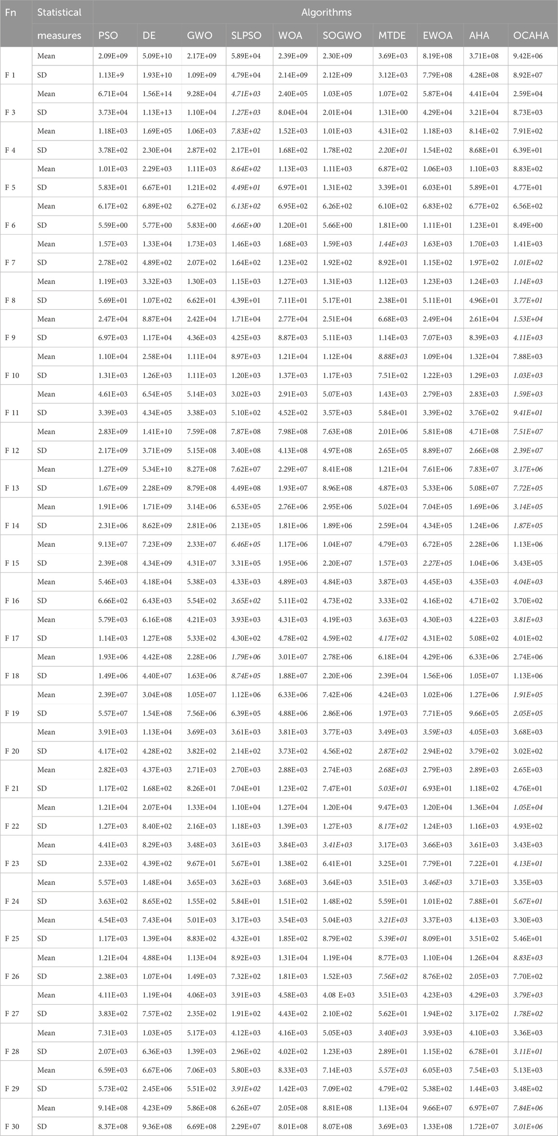
Table 4. Statistical results for the 29 unconstrained functions of CEC 2017 (50D, 30 runs).

Table 5

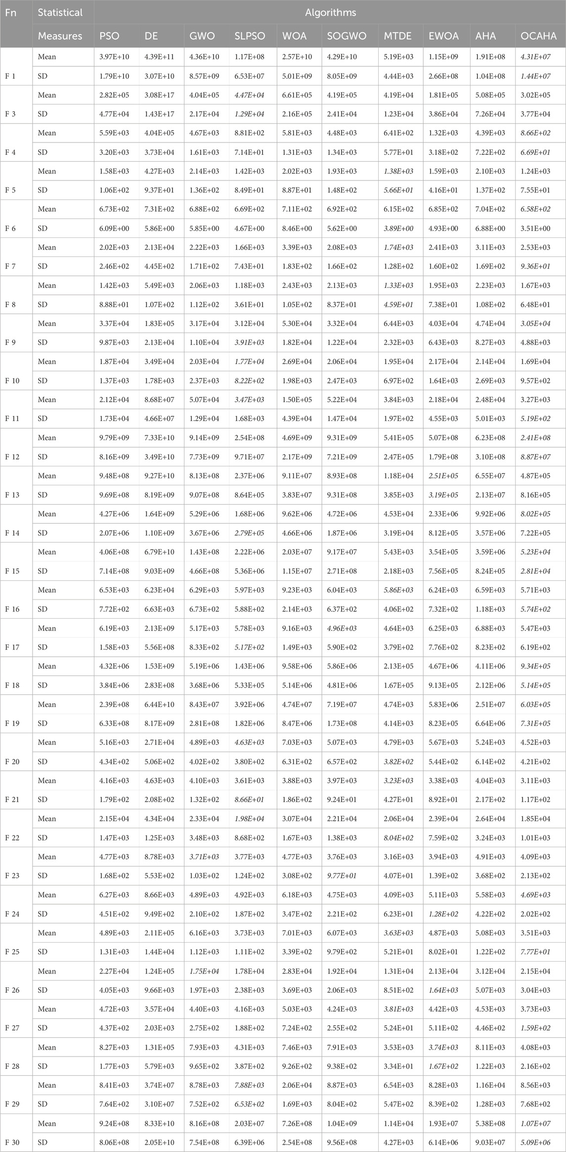
Table 5. Statistical results for the 29 unconstrained functions of CEC 2017 (100D, 30 runs).

Table 4 demonstrates that, of the 58 best performance indicators, 43 (22 Mean & 21 SD) have been achieved by MTDE, 10 (6 Mean & 4 SD) by OCAHA and the rest 5 (1 Mean & 4 SD) positions have been achieved by SLPSO. The same algorithms have achieved 13 (6 Mean & 7 SD), 27 (13 Mean & 14 SD) and 14 (7 Mean & 7 SD) positions respectively as the second best performer for the 50D set. For unimodal functions (F 1 and F 3), MTDE obtained outstanding optimized solutions followed by good solutions by SLPSO, and then the solutions of OCAHA come. For the multimodal category (F 4-F 10), MTDE achieved the minimum Mean for F 4, F 5, F 6, F 8 and F 9, and OCAHA obtained the same for the rest two functions F 7 and F 10. SLPSO achieved second best solution for F 4, F 5 and F 6 functions, and OCAHA achieved the second best solution for F 8 and F 9 functions. For the 10 hybrid functions (F 11-F 20), MTDE obtained almost all the best solutions, OCAHA obtained the second best mean fitness for F 11, F 12, F 13, F 14, F 16, F 17 and F 19 functions and the second best standard deviation for F 11, F 12, F 13, F 14 and F 19 functions. SLPSO achieved the second lowest mean value for F 15 and F 18 functions and EWOA achived the same for F 20 function. OCAHA results for the hybrid and the simple multimodal functions shows its better exploratory search ability than all the other algorithms except MTDE. MTDE emerges as the top performer among the 10 composition functions (F 21-F 30), providing the best Mean for F 22, F 23, F 26, F 27 and F 30 functions, OCAHA is the next performer with the lowest mean fitness value for F 21, F 24, F 28 and F 29 functions, and SLPSO obtained the same for F 25 function. The second best solution for mean fitness value for F 22, F 26, F 27 and F 30 functions and the second best value for standard deviation for F 23, F 24, F 27, F 28 and F 30 functions have been achieved by OCAHA. For composition functions, OCAHA solutions are competitive with respect to those of MTDE, and superior to all the other solutions for this simulation study with 50D set of CEC 2017 unconstrained benchmark functions. OCAHA’s performance on the composition functions demonstrates the algorithm’s strong local entrapment avoidance and its capacity to optimize complex real-world requirements.

Table 5 for 100D set demonstrates that, of the 58 best performance indicators, MTDE achieved 41 (18 Mean & 23 SD), OCAHA achieved 10 (9 Mean & 1 SD), SLPSO achieved 5 (2 Mean & 3 SD) and the rest 2 SD positions have been achieved by EWOA. The achieved positions among the 58 s best indicators are 12 (7 Mean & 5 SD) by MTDE, 23 (11 Mean & 12 SD) by OCAHA, 13 (6 Mean & 7 SD) by SLPSO, 6 (2 Mean & 4 SD) by EWOA, 2 (2 Mean) by GWO and 2 (1 Mean & 1 SD) by SOGWO. Comparing the results of 50D (Table 4) and 100D (Table 5), it is evident that, among the 9 100D functions with the best mean fitness solution by OCAHA, F 10 and F 21 are common to both dimensions with the best mean fitness solution by OCAHA, the functions F 5, F 11, F 16, F 20, F 22 and F 27 with the best mean fitness solution by MTDE for 50D, and the function F 25 with the best mean fitness solution by SLPSO. On the other side, in term of mean fitness solution, among the functions F 7, F 24, F 28 and F 29 with the best solution by OCAHA for 50D, MTDE ranked first for F 24, F 28 and F 29 for 100D. and SLPSO ranked first for the function F 7 for 100D. OCAHA obtained seventh, second, third and fifth ranked mean fitness solutions for the functions F 7, F 24, F 28 and F 29 respectively for 100D. OCAHA continues to provide the second best result for F 9, F 12, F 14, F 19 and F 30. In addition, OCAHA achieved the best standard deviation value for F 6 function, and the second best value of this statistical performance index for the functions F 1, F 4, F 7, F 11, F 12, F 15, F 16, F 18, F 19, F 25, F 27 and F 30. With 100D set, OCAHA continues to provide positive performance in the majority of its well performed 50D functions and achieved much better results in some new functions. The statistical results of 100D show that, the OCAHA’s optimizing performance is superior to all the comparing algorithms except MTDE, and the algorithm is capable of dealing with high-dimensional optimization problems.

At the 0.05 level of significance, the Wilcoxon test (WRST) (Wilcoxon, 1992) is performed to confirm the statistical importance of the OCAHA outcomes with regard to each participating result for each 100D function of the CEC 2017 test suite. p values are generated for each comparing pair between the OCAHA results and the participating algorithms’ results for each function. The WRST or Mann Whitney U test findings for OCAHA are shown in Table 6. A ‘+’ sign denotes the statistical importance between the verifying results, such as between OCAHA and its competitor, while a ‘$-$’ sign denotes no statistical significance between their outcomes, meaning that there is no statistical distinction between the two sets of results of a comparing combination. The Wilcoxon test results (Table 6) show that, OCAHA and SLPSO solutions are not statistically different from each other for the 8 functions: multimodal functions F 4, F 9 and F 1; hybrid functions F 11, F 12, F 16 and F 20; and 1 composition function F 28. The same observations of no statistical significance of the OCAHA results are found with PSO for F 3, F 9, F 26 and F 29, with GWO for F 9, F 15, F 17 and F 29, with EWOA for F 7, F 13, F 26 and F 29, with SOGWO for F 9, F 24 and F 29, and with MTDE for the function F 16. However, compared to its nine competitors, OCAHA achieved statistically significant outcomes in 91% of the 261 test measures, which proves the significant statistical advantages of the OCAHA optimized solutions.

Table 6

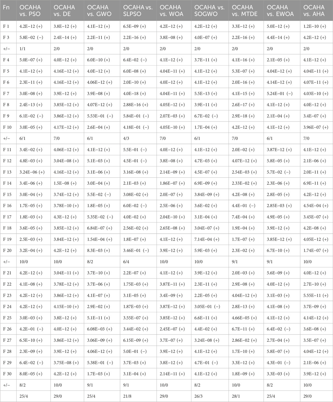
Table 6. Wilcoxon rank-sum test results for the 29 unconstrained functions of CEC 2017 (100D, 30 runs).

The present study has conducted the Friedman Mean Rank test (Friedman, 1937) (FMRT) to assess OCAHA’s overall performance and compare it to the other considered performances for both 50D and 100D functions of CEC 2017. The FMRT test rank of each method for each 100D function has been reported in Table 7, which shows that OCAHA stands first for 9 functions out of the 29 functions and second for 11 functions. The total optimization performance of all participating methods for both dimension sets can be visualized from Figure 3. As stated earlier, the developed multi-trial vector based approach (Nadimi-Shahraki et al., 2020) properly distributes the population between their subpopulations to enhance the search performance of MTDE, and this explains why the algorithm did better than any performance on the majority of the test functions of both dimensions. OCAHA achieved the second position with the Friedman mean ranks of 2.38 and 2.55 for 50D and 100D benchmark functions respectively. SLPSO has been found as the third best performer of this study with the mean ranks of 3.21 and 2.98 for 50D and 100D functions respectively, whereas the original PSO ranks eighth and seventh for these two dimensions of functions respectively. The performance of EWOA also reached to the fourth overall position with the mean ranks of 4.78 and 4.83 for 50D and 100D functions respectively, whereas its parent algorithm WOA stayed at the ninth position for both the dimensional sets of the benchmark functions. The performance of SOGWO has not been found satisfactory with respect to the original GWO performance for both the dimensions of the functions. However, OCAHA outperformed the original AHA in all the functions of both 50D and 100D.

Table 7

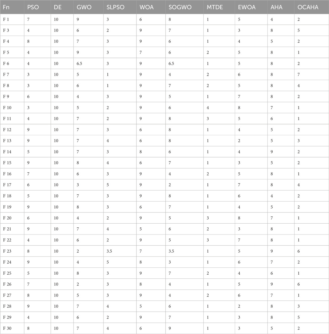
Table 7. Friedman test ranks for the 29 unconstrained functions of CEC 2017 (100D, 30 runs).

Figure 3

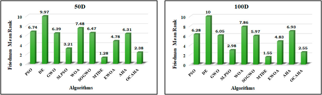
Figure 3. Friedman mean rank comparison plots for 50D and 100D CEC 2017 bencmark functions.

In Figure 4, the convergence profiles of OCAHA and 8 comparative methods for 1 unimodal (F 1), 2 multimodal (F 5 and F 10), 2 hybrid (F 15 and F 20) and 2 composition (F 22 and F 28) functions of 100-dimensional set of CEC 2017 have been drawn to evaluate the solving ability of OCAHA with respect to the steps of iterations, and to compare the same with the stated 8 algorithms including AHA. The mean of the best fitness values of 30 runs of each iteration of each algorithm has been considered to draw these convergence curves. For F 1, OCAHA shows the fastest convergence up to the first 50% of iterations and then slowly moves towards the better converged solution than all the other performers except MTDE. For F 5, F 10 and F 28, OCAHA reaches the fastest converged mean solution within the first 200 number of iterations and then finds more accuracy in the obtained solution in the later number of iterations, and obtains the best solution for F 5 and F 10 and 3rd best solution for F 28. For F 15, even though OCAHA does not show good convergence with respect to its competitors, like SLPSO, PSO, SOGWO, GWO, EWOA and even AHA up to the first 60% of iterations, it highly explores in the next 20% of iterations and converges into the second best solution after MTDE. For F 20 and F 22, OCAHA explores with a moderate convergence rate up to the first 40% of iterations and then updates its solution towards the global value for both the functions. OCAHA convergence profiles prove that the oppositional-chaotic approach has made the OCAHA methodology competitive with many leading algorithms in solving complex optimization problems.

Figure 4

Figure 4. Convergence profiles for CEC2017 (X-iterations, Y-means of best fitness values of each iteration).

4.2 Engineering design problems

In this phase, OCAHA has been studied on ten different engineering problems with mixed types of control or design variables and with the fulfilling requirements of both equality and inequality limitations of design. In all these engineering benchmark models, the present methodology is penalized with the high fitness value of a simple scalar penalty function to control the specified conditions of design constraints.

Population size and maximum iterations for each problem have been decided after some trial runs, and then for each problem, OCAHA CAHA and AHA (wherever required) have been implemented for 30 independent runs. Based on these 30 separate runs, the mean, best, worst and the standard deviation (SD) figures have been reported and have been compared with the available competing algorithms.

In the WBD optimization, a 50 population size and a 5,000 maximum function evaluations have been set for the algorithms AHA, CAHA and OCAHA. Table 8 shows the obtained optimized designs and its statistical comparison for the problem. To date, the best solution obtained for this model is the fitness function value of 1.955301 by PSO (real integer discrete coded) (Datta and Figueira, 2011) for a function evaluations number ranges from 19584 to 127848, and the same fitness value has been obtained by CAHA and OCAHA for 2,900 and 2,100 number of their function evaluations respectively. From the statistical comparison, OCAHA has been found to be the best and the most robust performer among all. Figure 5 for WBD problem presents the AHA, CAHA and OCAHA convergence profiles for the problem, where AHA reaches its solution of 1.958180 fitness function value at $92^{nd}$ iteration, CAHA achieves the best outcome for the problem, $i.e.1.955301$ fitness at its $58^{th}$ iterations, and OCAHA takes only $42^{nd}$ iterations to converge into the same solution.

Table 8

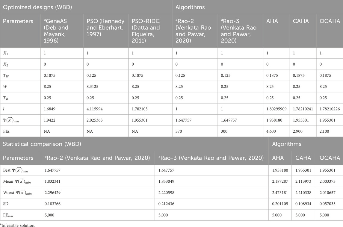
Table 8. Optimized designs and statistical comparison (WBD).

Figure 5

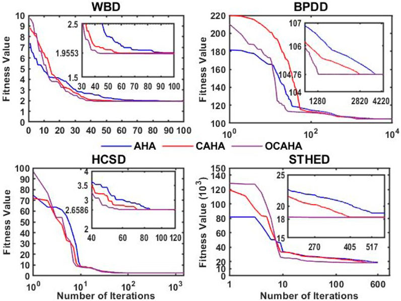
Figure 5. Convergence profiles of AHA, CAHA and OCAHA for WBD, BPDD, HCSD and STHED problems.

The considered population size and maximum function evaluations for the BPDD (Venkata Rao and Pawar, 2020, Thamaraikannan and Thirunavukkarasu, 2014) problem are 10 and 100000 respectively for the algorithms AHA, CAHA and OCAHA. Based on the 30 individual result sets, the OCAHA optimized designs and its statistical comparison for this problem have been reported in Table 9. Optimized designs of Table 9 clearly identifies OCAHA with the top feasible fitness function outcome of 104.761163 at the lowest computational cost of 12870 number of function evaluations. The average or mean, worst and the SD values in the statistical comparison of Table 9 proves the robustness quality of OCAHA solutions among all including CAHA and AHA. Figure 5 for BPDD problem presents the AHA, CAHA and OCAHA convergence profiles, where, AHA obtains its solution with the fitness function value of 104.761207 at the 4,216 iterations, CAHA achieves 104.761175 fitness after 2,812 iterations, and OCAHA converges into the best finding of the case at its $1287^{th}$ iteration.

Table 9

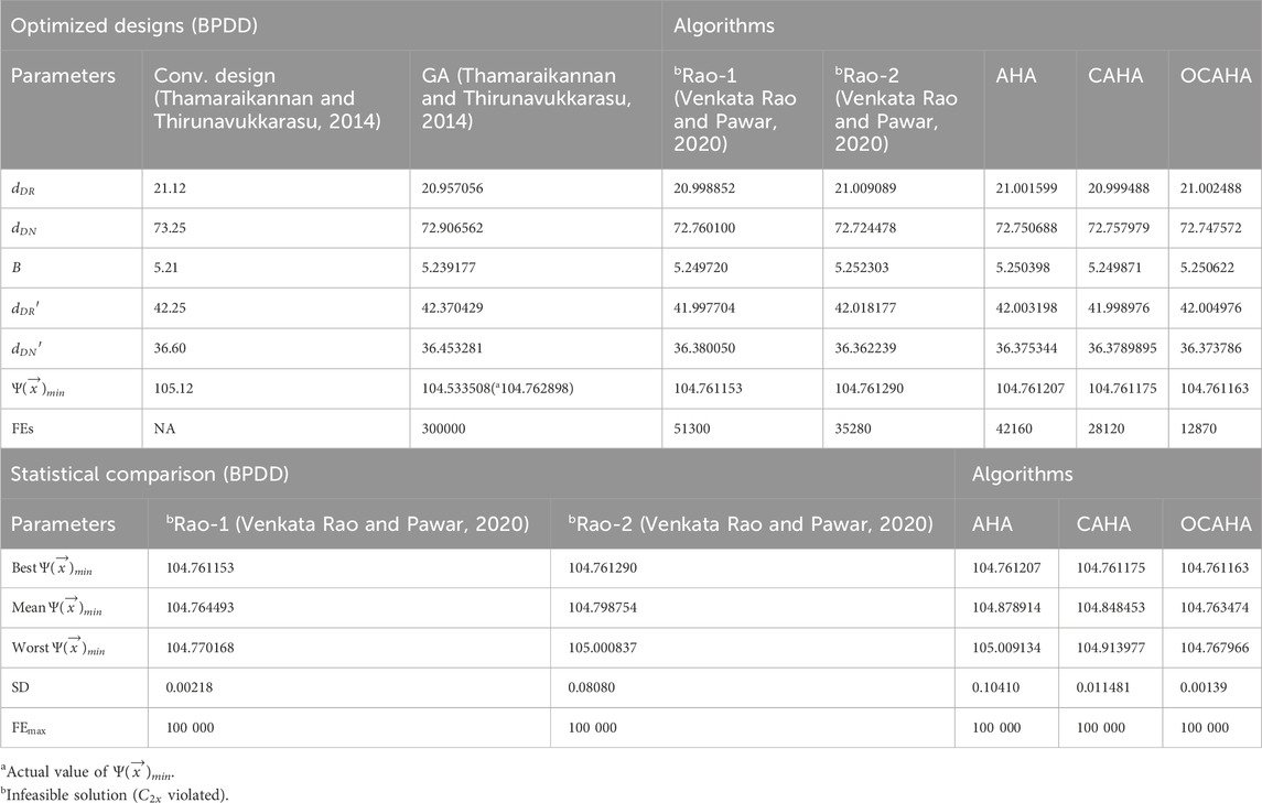
Table 9. Optimized designs and statistical comparison (BPDD).

A 50 population size and a 75000 maximum function evaluations were decided for AHA, CAHA and OCAHA for solving the HCSD weight minimization problem. The reported optimization of Table 10 shows that, the best optimized position with 2.658559 fitness value has been attained by PSO (RIDC) (Datta and Figueira, 2011) at the ‘4,784 to 98992’ range of function evaluations, by Rao-1 (Venkata Rao and Pawar, 2020) and Rao-2 (Venkata Rao and Pawar, 2020) at 45,400 & 25,000 number of function evaluations respectively, for AHA the required function evaluations number is 4,300, for CAHA 3650 function evaluations, and for OCAHA, this number is 2,850 only to reach the stated optimal solution. The statistical findings of Table 10 clearly identify the most robust performance of OCAHA among all. The AHA, CAHA and OCAHA convergence profiles of Figure 5 for the HCSD problem show that, AHA converges into the solution at its $86^{th}$ iteration, CAHA in its 73 iterations, and OCAHA takes 57 iterations to achieve the same.

Table 10

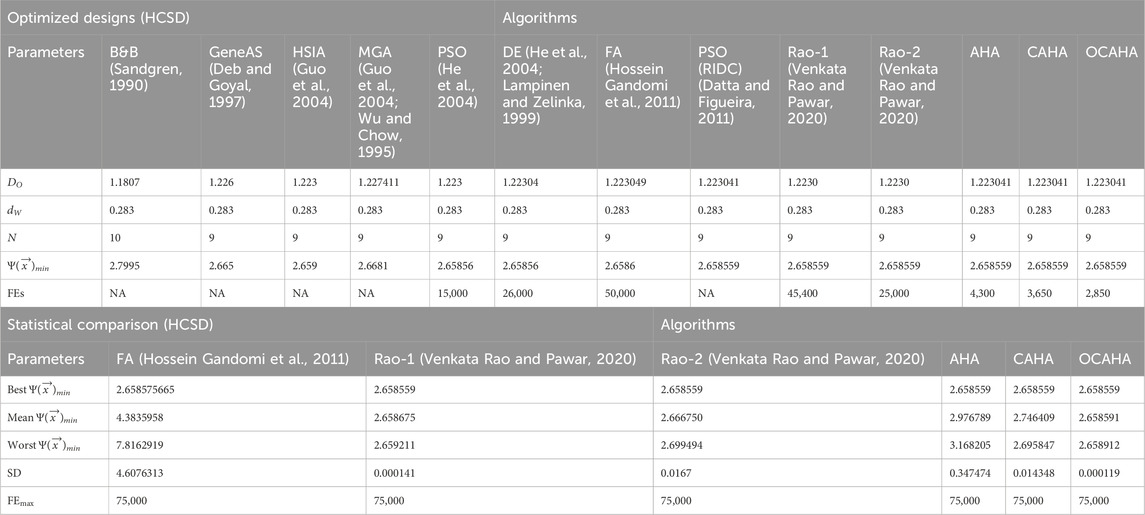
Table 10. Optimized designs and statistical comparison (HCSD).

For the HTBD (Siddall, 1982) design optimization problem, a 10 population size and for a close comparison with the available competing algorithms (Venkata Rao et al., 2011; Venkata Rao and Pawar, 2020, Zhao et al., 2022; He et al., 2004, Deb, 1997, Venkata Rao and Waghmare, 2017), a maximum 25000 function evaluations have been considered for implementing the algorithms CAHA and OCAHA. Table 11 of the optimized designs for the problem shows that, the best fitness of 1624.512578 has been achieved by OCAHA at the 22190 function evaluations and CAHA achieves 1624.516195 fitness at its 24180 function evaluations, whereas Rao-2 (Venkata Rao and Pawar, 2020) obtained 1625.184754 fitness value at its 24080 function evaluations. Statistical comparison part of Table 11 establishes the OCAHA algorithm as the most robust performer among all its competitors. Figure 6 for HTBD problem presents a statistical comparison plot for the obtained results by OCAHA and the other considered algorithms for the problem.

Table 11

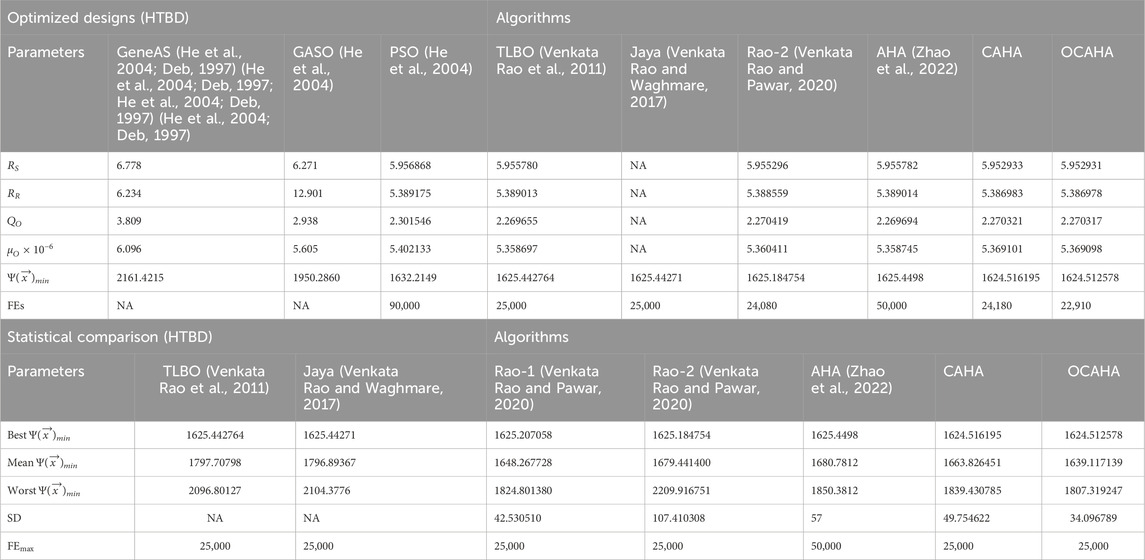
Table 11. Optimized designs and statistical comparison (HTBD).

Figure 6

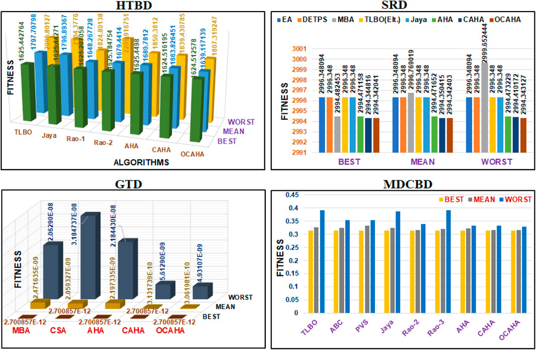
Figure 6. Statistical comparison plots for HTBD, SRD, GTD and MDCBD problems.

For the PVD problem, a 100 population size and a maximum 10000 function evaluations were fixed for AHA, CAHA and OCAHA methods. The reported optimized designs of Table 12 show that, the best fitness solution of 6059.70161 has been generated by EA (Mezura-Montes and Coello, 2005) at the computation of 30000 function evaluations, OCAHA secured the second position with a fitness value of 6059.71426316 after proceeding through its 4,300 function evaluations, CAHA ranked third with 6059.71427015 at its 5,600 function evaluations, AFA (Baykasoğlu and Ozsoydan, 2015) obtained the fourth best solution with a fitness value of 6059.71427196 at its 3,000 function evaluations approximately, and IPSO (He et al., 2004) performs with the fifth best design with 6059.7143 fitness value at the cost of its 30000 function evaluations. The statistical comparison of Table 12 for the obtained solutions of the problem indicates that, WAROA + JADE (Jiang et al., 2020) and TLBO (Venkata Rao et al., 2011) algorithms outperform all the algorithms including OCAHA in term of mean or average fitness result. However, compared to the WAROA + JADE algorithm, the OCAHA algorithm requires a significantly lower computing cost.

Table 12

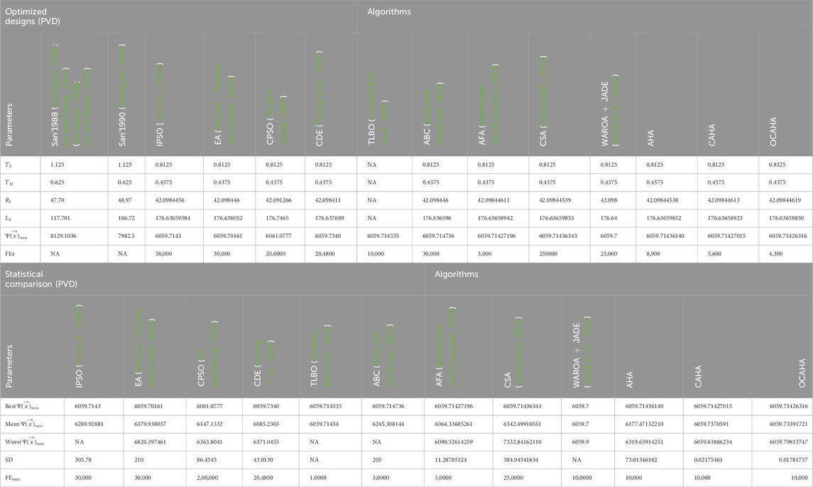
Table 12. Optimized designs and statistical comparison (PVD).

PFHED problem (Ramesh and Sekulic, 2003) considers seven designing variables and twenty two design inequality constraints to minimize the entropy generation units $N^{(s)}$ of a typical cross-flow (gas-to-air and single-pass) model of this system. The considered population size and maximum function evaluations for AHA, CAHA and OCAHA for the problem are 10 and 14000 respectively. Based on the 30 separate test-runs for all the three implementing methods, the optimized outcomes (Venkata Rao and Pawar, 2020; Zarea et al., 2014; Mariani et al., 2019; Ramesh and Sekulic, 2003) for this problem have been reported in Table 13. OCAHA obtains the best optimized fitness solution of 0.115402 at its 9,730 function evaluations. Rao-2 (Venkata Rao and Pawar, 2020) obtains 0.116546 and Rao-1 (Venkata Rao and Pawar, 2020) 0.116597 stand as the second and the third best designer for the problem respectively. FOA (Mariani et al., 2019) spends its 3,500 function evaluations in order to attain a comparatively faster convergence with a 0.1333 fitness value. Statistical comparison of Table 13 establishes that, for the same maximum function evaluations of 14000, OCAHA outperforms all the participating algorithms including AHA in all the performance indexes.

Table 13

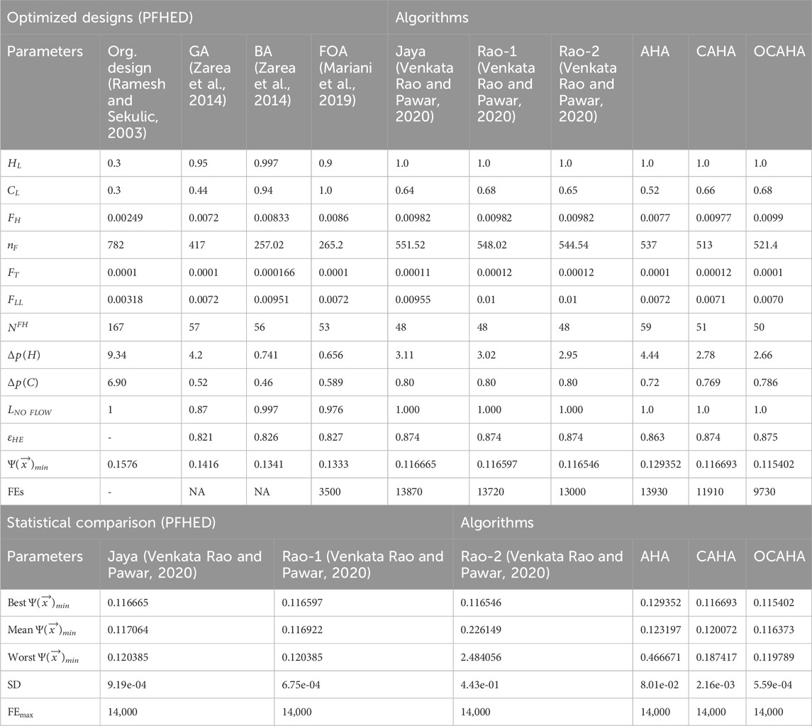
Table 13. Optimized designs and statistical comparison (PFHED).

The SRD problem requires weight minimization of a speed reducer. A population size of 100 has been decided to implement both CAHA and OCAHA algorithm for the problem. The designs optimized for this minimization problem have been outlined in Table 14. Table 14 demonstrates that, MBA (Ali et al., 2013) obtains a solution with 2,994.482453 fitness function value at the cost of its 6300 function evaluations, AHA (Zhao et al., 2022) solves the problem with a fitness value of 2,994.471158 after proceeding through its 30000 function evaluations, CAHA generates 2,994.344816 fitness solution at its 7,200 function evaluations, and OCAHA obtains the best fitness value of 2,994.342041 im its 6900 number of function evaluations. With respect to the required computational cost, $i.e$ the function evaluations in optimizing the problem in marginal deviation, MBA outperforms all the reported algorithms including OCAHA. Statistical comparison of Table 14 shows that, the best, mean or average and the worst values of OCAHA solutions are best among all, whereas, Jaya (Venkata Rao and Waghmare, 2017) and CAHA algorithms outperform OCAHA with the standard deviation (SD) values of 0 and $5.37\times {10}^{-5}$, respectively for the same number of maximum function evaluations 10000. The statistical comparison plot in Figure 6 for the SRD problem clearly identifies the robustness solving ability of OCAHA among all the considered competing algorithms.

Table 14

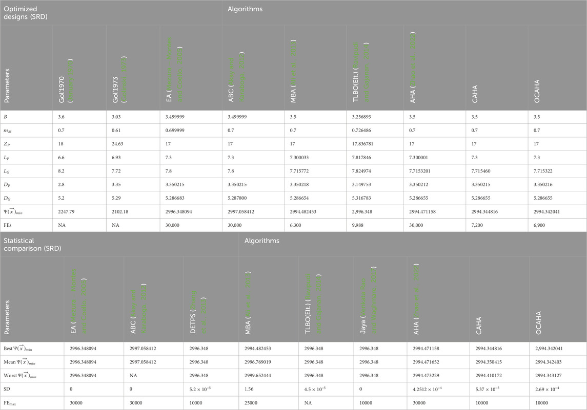
Table 14. Optimized designs and statistical comparison (SRD).

In the STHED (Kern and Kern, 1950) problem, three control or designing variables have been considered along with eight inequality constraints for the total annual cost $C_T$ minimization of a shell and tube model of heat exchanger. A 10 population size and a maximum 6000 function evaluations are the decided algorithmic parameters for all the three methods (AHA, CAHA and OCAHA) to optimize the problem, and based on the 30 individual result sets, the obtained designs have been compared with the available designs from literature as reported in Table 15. OCAHA outperforms all the algorithms (Venkata Rao and Pawar, 2020; Mariani et al., 2019; Kern and Kern, 1950; Caputo et al., 2008; Amin and Ali, 2013; Patel and Rao, 2010) with a fitness function value of 18240.94 at the cost of its 2,700 number of function evaluations. CAHA ranks second with the fitness solution of 18285.31 at the cost of its 4,050 function evaluations. Rao-1 and 3 (Venkata Rao and Pawar, 2020), both the algorithms with the same fitness result of 18335.99 and FOA (Mariani et al., 2019) with 18560.3 rank third, fourth, and fifth performers, respectively for this minimizing optimization case. With just 350 function evaluations, PSO (Patel and Rao, 2010) achieved the fastest converged solution with a 20310 fitness value. Statistical comparison of Table 15 clearly shows that the Rao-1 (Venkata Rao and Pawar, 2020) method achieves the most robust optimization with the standard deviation of 5.77e-02, whereas, OCAHA outperforms all the participating algorithms including Rao-1 in the remaining comparing indexes. Convergence profiles of Figure 5 for STHED problem show that, the AHA reaches the 18926.45 fitness value at its 517 number of iterations and CAHA achieves 18285.31 after 405 iterations, whereas, with a faster rate of convergence, OCAHA obtains the best solution at its $270^{th}$ iteration.

Table 15

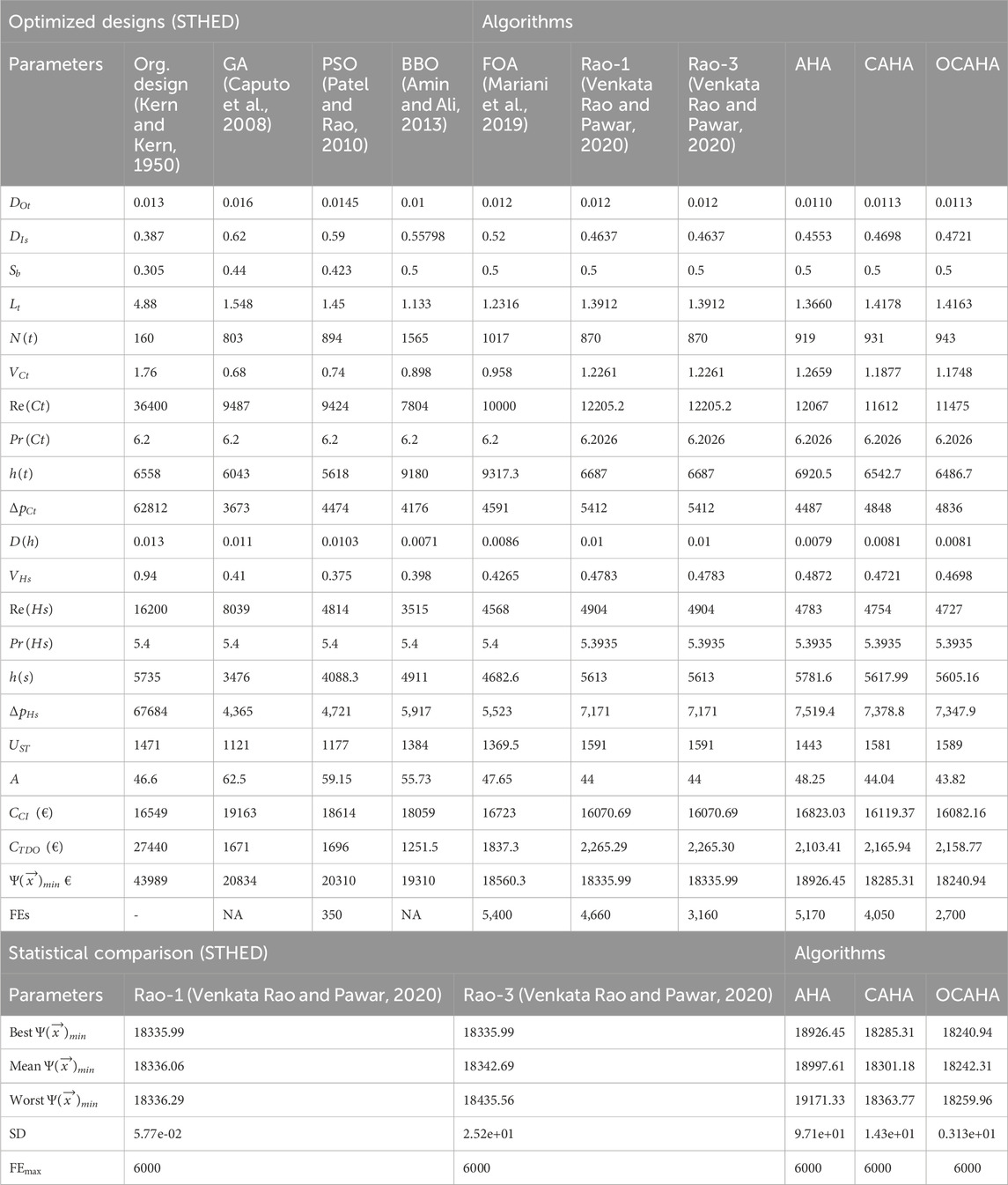
Table 15. Optimized designs and statistical comparison (STHED).

The GTD is an unconstrained minimization problem, which optimizes four number integer type control or designing variables to minimize the problem objective. A 50 population has been considered for AHA, CAHA and OCAHA to solve this problem. The obtained optimized designs (Table 16) show that, the ABC (Akay and Karaboga, 2012) algorithm obtains the global solution with $2.700857\times {10}^{-12}$ fitness function value at the lowest computational cost of only its 60 function evaluations among all. OCAHA comes out as the second performer in this regard with 350 number of its function evaluations to converge into the stated global solution. CAHA takes its 450 function evaluations to reach the same solution for this case. Statistical comparison of Table 16 shows that, the average or mean, worst and the SD measures of OCAHA results are the best of all the participating methods including ABC (Akay and Karaboga, 2012). However, ABC employed a maximum of 30000 function evaluations, whereas, for MBA (Ali et al., 2013), CSA (Askarzadeh, 2016), AHA, CAHA and OCAHA algorithms, a maximum of 10000 function evaluations have been considered to obtain the reported results. Statistical comparison plot of Figure 6 for GTD problem clearly identifies OCAHA and CAHA as the first and the second robust performers for the case respectively among all.

Table 16

Table 16. Optimized designs and statistical comparison (GTD).

The applied population size in the MDCBD problem for CAHA and OCAHA for mass minimization of a multiple disc clutch brake system is 5. Table 17 demonstrates that, OCAHA obtains the so far lowest solution (0.3136566) with the optimized actuating force $(P_A)$ of 800 at its $105^{th}$ function evaluations. CAHA achieves the same set of solution at the cost of its 125 function evaluations. Statistical comparison of Table 17 reveals that, for the same number (600) of maximum function evaluations, the average or mean, worst and the standard deviation measures of OCAHA solutions are best among all. Statistical plot of Figure 6 for MDCBD clearly identifies the OCAHA algorithm for its most robust performance parameters for the problem.

Table 17

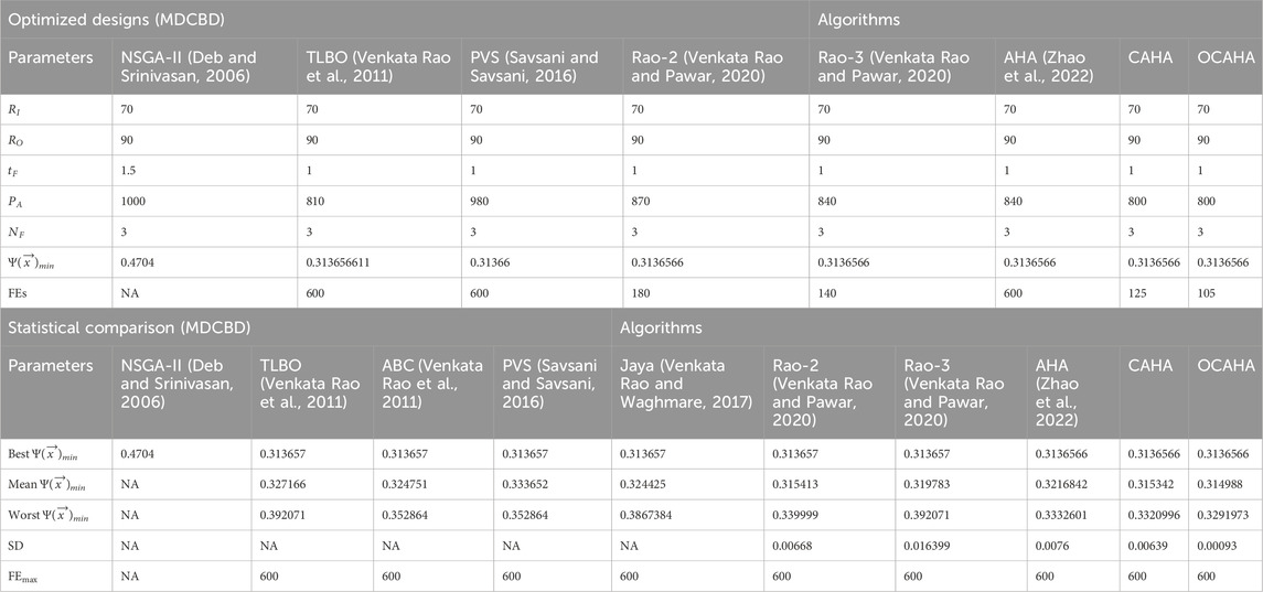
Table 17. Optimized designs and statistical comparison (MDCBD).

5 Conclusion

This work modified the newly designed AHA methodology by the OBL rule and the chaos of Gauss/mouse map for more accurate and faster optimization. The proposed OCAHA method has been tested on 50 and 100 dimensional sets of the unconstrained CEC 2017 benchmark suite, and on the 10 challenging models of engineering optimization. Four state of the art optimizers, viz. PSO, DE, GWO and WOA, their recently developed 4 effective variants, viz. SLPSO, MTDE, SOGWO and EWOA, and AHA have been the participating algorithms benchmarked on CEC 2017 functions to evaluate the overall optimization performance of OCAHA. OCAHA performance parameters for the engineering problems have been compared with the leading algorithms of literature to verify its applicability in the complex real-world cases of optimization.

Statistical assessment of the CEC 2017 results through the standard indexes and tests (WRST and FMRT), and the convergence profiles identify OCAHA as the second performer of the evaluation after MTDE. The OCAHA optimized designs for engineering cases have been found superior to the previous performances. In the engineering design optimizations, on average, it has reduced the computational cost by 57.5% and 22.63% in term of function evaluations and the fitness value by 2.4% and 0.23% in comparison to the parent method AHA and its chaotic version CAHA, respectively. Overall, the study justifies modifying AHA with the proposed strategy, and confirms its potential to compete with many leading optimizers in dealing with the practical complexities.

In the future works, (a) the present method can be applied for the other challenging problems of engineering optimization, (b) the methodology can be equipped with the appropriate enhancers for more effectiveness, (c) it can be enabled for the current and more complex aspects of engineering and for real data optimization, and for the ongoing applications of machine learning, (c) the multi-objective algorithmic form of OCAHA can be implemented.

Data availability statement

The raw data supporting the conclusions of this article will be made available by the authors, without undue reservation.

Author contributions

VB: Writing – original draft, Writing – review and editing, Conceptualization, Data curation, Formal Analysis, Funding acquisition, Investigation, Methodology, Project administration, Resources, Software, Supervision, Validation, Visualization. PR: Writing – original draft, Writing – review and editing, Conceptualization, Data curation, Formal Analysis, Funding acquisition, Investigation, Methodology, Project administration, Resources, Software, Supervision, Validation, Visualization. GT: Conceptualization, Methodology, Writing – review and editing, Data curation, Formal Analysis, Funding acquisition, Investigation, Project administration, Resources, Software, Supervision, Validation, Visualization. SM: Writing – review and editing, Conceptualization, Data curation, Formal Analysis, Funding acquisition, Investigation, Methodology, Project administration, Resources, Software, Supervision, Validation, Visualization.

Funding

The author(s) declare that no financial support was received for the research and/or publication of this article.

Conflict of interest

The authors declare that the research was conducted in the absence of any commercial or financial relationships that could be construed as a potential conflict of interest.

Generative AI statement

The authors declare that no Generative AI was used in the creation of this manuscript.

Publisher’s note

All claims expressed in this article are solely those of the authors and do not necessarily represent those of their affiliated organizations, or those of the publisher, the editors and the reviewers. Any product that may be evaluated in this article, or claim that may be made by its manufacturer, is not guaranteed or endorsed by the publisher.

References

Aasim, M., Katırcı, R., Akgur, O., Yildirim, B., Mustafa, Z., Nadeem, M. A., et al. (2022). Machine learning (ml) algorithms and artificial neural network for optimizing in vitro germination and growth indices of industrial hemp (cannabis sativa l.). Industrial Crops Prod. 181, 114801. doi:10.1016/j.indcrop.2022.114801

CrossRef Full Text | Google Scholar

Abbassi, R., Abbassi, A., Heidari, A. A., and Mirjalili, S. (2019). An efficient salp swarm-inspired algorithm for parameters identification of photovoltaic cell models. Energy Convers. Manag. 179, 362–372. doi:10.1016/j.enconman.2018.10.069

CrossRef Full Text | Google Scholar

Agrawal, S., Panda, R., Choudhury, P., and Abraham, A. (2022). Dominant color component and adaptive whale optimization algorithm for multilevel thresholding of color images. Knowledge-Based Syst. 240, 108172. doi:10.1016/j.knosys.2022.108172

CrossRef Full Text | Google Scholar

Ahmad Rather, S., and Shanthi Bala, P. (2020). Swarm-based chaotic gravitational search algorithm for solving mechanical engineering design problems. World J. Eng. 17, 97–114. doi:10.1108/wje-09-2019-0254

CrossRef Full Text | Google Scholar

Akay, B., and Karaboga, D. (2012). Artificial bee colony algorithm for large-scale problems and engineering design optimization. J. intelligent Manuf. 23 (4), 1001–1014. doi:10.1007/s10845-010-0393-4

CrossRef Full Text | Google Scholar

Ali, S., Bahreininejad, A., Eskandar, H., and Hamdi, M. (2013). Mine blast algorithm: a new population based algorithm for solving constrained engineering optimization problems. Appl. Soft Comput. 13 (5), 2592–2612. doi:10.1016/j.asoc.2012.11.026

CrossRef Full Text | Google Scholar

Amin, H., and Ali, N. (2013). Design and economic optimization of shell-and-tube heat exchangers using biogeography-based (bbo) algorithm. Appl. Therm. Eng. 51 (1-2), 1263–1272. doi:10.1016/j.applthermaleng.2012.12.002

CrossRef Full Text | Google Scholar

Askarzadeh, A. (2016). A novel metaheuristic method for solving constrained engineering optimization problems: crow search algorithm. Comput. and Struct. 169, 1–12. doi:10.1016/j.compstruc.2016.03.001

CrossRef Full Text | Google Scholar

Awad, N. H., Ali, M. Z., Suganthan, P. N., Liang, J. J., and Qu, B. Y. (2017). Problem definitions and evaluation criteria for the cec2017. Special Sess. Compet. Single Objective Param. Numer. Optim.

Google Scholar

Awad, R. (2021). Sizing optimization of truss structures using the political optimizer (po) algorithm. Structures 33, 4871–4894. doi:10.1016/j.istruc.2021.07.027

CrossRef Full Text | Google Scholar

Baykasoğlu, A., and Ozsoydan, F. B. (2015). Adaptive firefly algorithm with chaos for mechanical design optimization problems. Appl. soft Comput. 36, 152–164. doi:10.1016/j.asoc.2015.06.056

CrossRef Full Text | Google Scholar

Burcin Ozsoydan, F., and Baykasoglu, A. (2021). Chaos and intensification enhanced flower pollination algorithm to solve mechanical design and unconstrained function optimization problems. Expert Syst. Appl. 184, 115496. doi:10.1016/j.eswa.2021.115496

CrossRef Full Text | Google Scholar

Cajori, F. (1999). A history of mathematics. Am. Math. Soc. 303.

Google Scholar

Caputo, A. C., Pelagagge, P. M., and Salini, P. (2008). Heat exchanger design based on economic optimisation. Appl. Therm. Eng. 28 (10), 1151–1159. doi:10.1016/j.applthermaleng.2007.08.010

CrossRef Full Text | Google Scholar

Chauhan, S., Vashishtha, G., Zimroz, R., Kumar, R., and Gupta, M. K. (2024). Optimal filter design using mountain gazelle optimizer driven by novel sparsity index and its application to fault diagnosis. Appl. Acoust. 225, 110200. doi:10.1016/j.apacoust.2024.110200

CrossRef Full Text | Google Scholar

Cheng, M.-Y., and Prayogo, D. (2017). A novel fuzzy adaptive teaching–learning-based optimization (fatlbo) for solving structural optimization problems. Eng. Comput. 33 (1), 55–69. doi:10.1007/s00366-016-0456-z

CrossRef Full Text | Google Scholar

Cheng, R., and Jin, Y. (2015). A social learning particle swarm optimization algorithm for scalable optimization. Inf. Sci. 291, 43–60. doi:10.1016/j.ins.2014.08.039

CrossRef Full Text | Google Scholar

Datta, D., and Figueira, J. R. (2011). A real-integer-discrete-coded particle swarm optimization for design problems. Appl. Soft Comput. 11 (4), 3625–3633. doi:10.1016/j.asoc.2011.01.034

CrossRef Full Text | Google Scholar

Deb, K. (1997). Geneas: a robust optimal design technique for mechanical component design. Evol. algorithms Eng. Appl., 497–514. doi:10.1007/978-3-662-03423-1_27

CrossRef Full Text | Google Scholar

Deb, K., and Goyal, M. (1997). “Optimizing engineering designs using a combined genetic search,” in Icga (Citeseer), 521–528.

Google Scholar

Deb, K., and Goyal, M. (1996). A combined genetic adaptive search (geneas) for engineering design. Comput. Sci. Inf. 26, 30–45.

Google Scholar

Deb, K., and Srinivasan, A. (2006). Innovization: innovating design principles through optimization. Available online at: https://scholar.google.com/scholar?hl=en&as_sdt=0%2C5&q=Innovization%3A+Innovating+design+principles+through+optimization&btnG=.

Google Scholar

Deng, Y., Liu, Y., Zeng, R., Wang, Q., Li, Z., Zhang, Y., et al. (2021). A novel operation strategy based on black hole algorithm to optimize combined cooling, heating, and power-ground source heat pump system. Energy 229, 120637. doi:10.1016/j.energy.2021.120637

CrossRef Full Text | Google Scholar

Dhargupta, S., Ghosh, M., Mirjalili, S., and Sarkar, R. (2020). Selective opposition based grey wolf optimization. Expert Syst. Appl. 151, 113389. doi:10.1016/j.eswa.2020.113389

CrossRef Full Text | Google Scholar

El-Abbasy, M. S., Elazouni, A., and Zayed, T. (2020). Finance-based scheduling multi-objective optimization: benchmarking of evolutionary algorithms. Automation Constr. 120, 103392. doi:10.1016/j.autcon.2020.103392

CrossRef Full Text | Google Scholar

Fan, Q., Huang, H., Yang, K., Zhang, S., Yao, L., and Xiong, Q. (2021). A modified equilibrium optimizer using opposition-based learning and novel update rules. Expert Syst. Appl. 170, 114575. doi:10.1016/j.eswa.2021.114575

CrossRef Full Text | Google Scholar

Faris, H., Ala’M, A.-Z., Ali, A. H., Aljarah, I., Mafarja, M., Hassonah, M. A., et al. (2019). An intelligent system for spam detection and identification of the most relevant features based on evolutionary random weight networks. Inf. Fusion 48, 67–83. doi:10.1016/j.inffus.2018.08.002

CrossRef Full Text | Google Scholar

Friedman, M. (1937). The use of ranks to avoid the assumption of normality implicit in the analysis of variance. J. Am. Stat. Assoc. 32 (200), 675–701. doi:10.2307/2279372

CrossRef Full Text | Google Scholar

George, G. (1956). Minimum weight analysis of compression structures. New York University Press New York, NY.

Google Scholar

Ghasemi, M., Akbari, E., Zand, M., Hadipour, M., Ghavidel, S., and Li, L. (2019). An efficient modified hpso-tvac-based dynamic economic dispatch of generating units. Electr. Power Components Syst. 47 (19-20), 1826–1840. doi:10.1080/15325008.2020.1731876

CrossRef Full Text | Google Scholar

Goldberg, D. E. (2006). Genetic algorithms. Pearson Education India Chennai.

Google Scholar

Golinski, J. (1973). An adaptive optimization system applied to machine synthesis. Mech. Mach. Theory 8 (4), 419–436. doi:10.1016/0094-114x(73)90018-9

CrossRef Full Text | Google Scholar

Gu, C., Zhu, D., and Pei, Y. (2018). A new inexact sqp algorithm for nonlinear systems of mixed equalities and inequalities. Numer. Algorithms 78 (4), 1233–1253. doi:10.1007/s11075-017-0421-y

CrossRef Full Text | Google Scholar

Guan, G., Zhang, X., Wang, P., and Yang, Q. (2022). Multi-objective optimization design method of marine propeller based on fluid-structure interaction. Ocean. Eng. 252, 111222. doi:10.1016/j.oceaneng.2022.111222

CrossRef Full Text | Google Scholar

Guo, C. X, Hu, J. S, Ye, B., and Cao, Y. J. (2004). Swarm intelligence for mixed-variable design optimization. J. Zhejiang University-Science A 5 (7), 851–860. doi:10.1631/jzus.2004.0851

PubMed Abstract | CrossRef Full Text | Google Scholar

Hamid, R. T. (2005). Opposition-based learning: a new scheme for machine intelligence. Int. Conf. Comput. Intell. Model. Control Automation Int. Conf. Intelligent Agents, Web Technol. Internet Commer. (CIMCA-IAWTIC’06) 1, 695–701.

Google Scholar

He, Q., and Wang, L. (2007). An effective co-evolutionary particle swarm optimization for constrained engineering design problems. Eng. Appl. Artif. Intell. 20 (1), 89–99. doi:10.1016/j.engappai.2006.03.003

CrossRef Full Text | Google Scholar

He, S., Prempain, E., and Wu, Q. H. (2004). An improved particle swarm optimizer for mechanical design optimization problems. Eng. Optim. 36 (5), 585–605. doi:10.1080/03052150410001704854

CrossRef Full Text | Google Scholar

Hossein Gandomi, A., Yang, X.-S., and Alavi, A. H. (2011). Mixed variable structural optimization using firefly algorithm. Comput. and Struct. 89 (23-24), 2325–2336. doi:10.1016/j.compstruc.2011.08.002

CrossRef Full Text | Google Scholar

Hossein Gandomi, A., Yun, G. J., Yang, X.-S., and Talatahari, S. (2013). Chaos-enhanced accelerated particle swarm optimization. Commun. Nonlinear Sci. Numer. Simul. 18 (2), 327–340. doi:10.1016/j.cnsns.2012.07.017

CrossRef Full Text | Google Scholar

Huang, F. Z., Wang, L., and He, Q. (2007). An effective co-evolutionary differential evolution for constrained optimization. Appl. Math. Comput. 186 (1), 340–356. doi:10.1016/j.amc.2006.07.105

CrossRef Full Text | Google Scholar

Jan, G. (1970). Optimal synthesis problems solved by means of nonlinear programming and random methods. J. Mech. 5 (3), 287–309. doi:10.1016/0022-2569(70)90064-9

CrossRef Full Text | Google Scholar

Jena, S., Jeet, S., Kumar Bagal, D., Kumar Baliarsingh, A., Nayak, D. R., and Barua, A. (2022). Efficiency analysis of mechanical reducer equipment of material handling industry using sunflower optimization algorithm and material generation algorithm. Mater. Today Proc. 50, 1113–1122. doi:10.1016/j.matpr.2021.08.005

CrossRef Full Text | Google Scholar

Jiang, R., Yang, M., Wang, S., and Chao, T. (2020). An improved whale optimization algorithm with armed force program and strategic adjustment. Appl. Math. Model. 81, 603–623. doi:10.1016/j.apm.2020.01.002

CrossRef Full Text | Google Scholar

Jordán, J., Palanca, J., Martí, P., and Julian, V. (2022). Electric vehicle charging stations emplacement using genetic algorithms and agent-based simulation. Expert Syst. Appl. 197, 116739. doi:10.1016/j.eswa.2022.116739

CrossRef Full Text | Google Scholar

Jothiprakash, V., and Arunkumar, R. (2013). Optimization of hydropower reservoir using evolutionary algorithms coupled with chaos. Water Resour. Manag. 27, 1963–1979. doi:10.1007/s11269-013-0265-8

CrossRef Full Text | Google Scholar

Kasprzak, E. M., and Lewis, K. E. (2001). Pareto analysis in multiobjective optimization using the collinearity theorem and scaling method. Struct. Multidiscip. Optim. 22 (3), 208–218. doi:10.1007/s001580100138

CrossRef Full Text | Google Scholar

Kennedy, J., and Eberhart, R. (1995). Particle swarm optimization. Proc. ICNN’95-international Conf. neural Netw. 4, 1942–1948. doi:10.1109/icnn.1995.488968

CrossRef Full Text | Google Scholar

Kennedy, J., and Eberhart, R. C. (1997). A discrete binary version of the particle swarm algorithm. 1997 IEEE Int. Conf. Syst. man, Cybern. Comput. Cybern. Simul. 5, 4104–4108. doi:10.1109/icsmc.1997.637339

CrossRef Full Text | Google Scholar

Kern, D. Q., and Kern, D. Q. (1950). Process heat transfer, 871. New York: McGraw-Hill.

Google Scholar

Khac Truong, T., Li, K., and Xu, Y. (2013). Chemical reaction optimization with greedy strategy for the 0–1 knapsack problem. Appl. soft Comput. 13 (4), 1774–1780. doi:10.1016/j.asoc.2012.11.048

CrossRef Full Text | Google Scholar

Lampinen, J., and Zelinka, I. (1999). Mixed integer-discrete-continuous optimization by differential evolution. Available online at: https://scholar.google.com/scholar?hl=en&as_sdt=0%2C5&q=Mixed+integer-discrete-continuous+optimization+by+differential+evolution&btnG=.

Google Scholar

Lee, K. S., and Geem, Z. W. (2005). A new meta-heuristic algorithm for continuous engineering optimization: harmony search theory and practice. Comput. methods Appl. Mech. Eng. 194 (36-38), 3902–3933. doi:10.1016/j.cma.2004.09.007

CrossRef Full Text | Google Scholar

Liu, Z. S., and Li, S. (2018). Whale optimization algorithm based on chaotic sine cosine operator. Comput. Eng. Appl. 54 (7), 159–163.

Google Scholar

Mariani, V. C., Coelho, L. dos S., and Coelho, L. d. S. (2019). Design of heat exchangers using falcon optimization algorithm. Appl. Therm. Eng. 156, 119–144. doi:10.1016/j.applthermaleng.2019.04.038

CrossRef Full Text | Google Scholar

Mezura-Montes, E., and Coello, C. A. C. (2005). “Useful infeasible solutions in engineering optimization with evolutionary algorithms,” in Mexican international conference on artificial intelligence (Springer), 652–662.

Google Scholar

Mirjalili, S., and Lewis, A. (2016). The whale optimization algorithm. Adv. Eng. Softw. 95, 51–67. doi:10.1016/j.advengsoft.2016.01.008

CrossRef Full Text | Google Scholar

Mirjalili, S., Mirjalili, S. M., and Lewis, A. (2014). Grey wolf optimizer. Adv. Eng. Softw. 69, 46–61. doi:10.1016/j.advengsoft.2013.12.007

CrossRef Full Text | Google Scholar

Nadimi-Shahraki, M. H., Taghian, S., Mirjalili, S., and Faris, H. (2020). Mtde: an effective multi-trial vector-based differential evolution algorithm and its applications for engineering design problems. Appl. Soft Comput. 97, 106761. doi:10.1016/j.asoc.2020.106761

CrossRef Full Text | Google Scholar

Okulewicz, M., and Mańdziuk, J. (2019). A metaheuristic approach to solve dynamic vehicle routing problem in continuous search space. Swarm Evol. Comput. 48, 44–61. doi:10.1016/j.swevo.2019.03.008

CrossRef Full Text | Google Scholar

Om Prakash, S., Jeyakumar, M., and Gandhi, B. S. (2022). Parametric optimization on electro chemical machining process using pso algorithm. Mater. Today Proc. 62, 2332–2338. doi:10.1016/j.matpr.2022.04.141

CrossRef Full Text | Google Scholar

Osman, K. E., and Eksin, I. (2006). A new optimization method: big bang–big crunch. Adv. Eng. Softw. 37 (2), 106–111. doi:10.1016/j.advengsoft.2005.04.005

CrossRef Full Text | Google Scholar

Patel, V. K., and Rao, R. V. (2010). Design optimization of shell-and-tube heat exchanger using particle swarm optimization technique. Appl. Therm. Eng. 30 (11-12), 1417–1425. doi:10.1016/j.applthermaleng.2010.03.001

CrossRef Full Text | Google Scholar

Pavanu Sai, J., and Rao, B. N. (2022). Non-dominated sorting genetic algorithm ii and particle swarm optimization for design optimization of shell and tube heat exchanger. Int. Commun. Heat Mass Transf. 132, 105896. doi:10.1016/j.icheatmasstransfer.2022.105896

CrossRef Full Text | Google Scholar

Peitgen, H.-O., Jürgens, H., and Saupe, D. (1992). “Strange attractors: the locus of chaos,” in Chaos and fractals (Springer), 655–768.

Google Scholar

Petcharaks, N., and Ongsakul, W. (2007). Hybrid enhanced Lagrangian relaxation and quadratic programming for hydrothermal scheduling. Electr. Power Components Syst. 35 (1), 19–42. doi:10.1080/15325000600815449

CrossRef Full Text | Google Scholar

Qiao, W., Moayedi, H., and Kok Foong, L. (2020). Nature-inspired hybrid techniques of iwo, da, es, ga, and ica, validated through a k-fold validation process predicting monthly natural gas consumption. Energy Build. 217, 110023. doi:10.1016/j.enbuild.2020.110023

CrossRef Full Text | Google Scholar

Qiao, W., and Yang, Z. (2019). Modified dolphin swarm algorithm based on chaotic maps for solving high-dimensional function optimization problems. IEEE Access 7, 110472–110486. doi:10.1109/access.2019.2931910

CrossRef Full Text | Google Scholar

Rafi, V., and Dhal, P. K. (2020). Maximization savings in distribution networks with optimal location of type-I distributed generator along with reconfiguration using PSO-DA optimization techniques. Mater. Today Proc. 33, 4094–4100. doi:10.1016/j.matpr.2020.06.547

CrossRef Full Text | Google Scholar

Rahnamayan, S., Tizhoosh, H. R., and Salama, M. M. A. (2008). Opposition versus randomness in soft computing techniques. Appl. Soft Comput. 8 (2), 906–918. doi:10.1016/j.asoc.2007.07.010

CrossRef Full Text | Google Scholar

Rajendra Prasad, V., and Kuo, W. (2000). Reliability optimization of coherent systems. IEEE Trans. Reliab. 49 (3), 323–330. doi:10.1109/24.914551

CrossRef Full Text | Google Scholar

Rajesh, A., Ashoka Varthanan, P., Srikant, J., Shoban, T., Sanjaykanna, K. S., and Suchith, P. V. (2021). Optimization of shot peening process parameters using pso algorithm to maximise the fatigue strength, flexural strength and surface hardness of aa2024-t3 alloy. Mater. Today Proc.

Google Scholar

Ramesh, K. S., and Sekulic, D. P. (2003). Fundamentals of heat exchanger design. John Wiley and Sons.

Google Scholar

Rashedi, E., Nezamabadi-Pour, H., and Saryazdi, S. (2009). Gsa: a gravitational search algorithm. Inf. Sci. 179 (13), 2232–2248. doi:10.1016/j.ins.2009.03.004

CrossRef Full Text | Google Scholar

Ravipudi, V. R., and Gajanan, G. W. (2014). Complex constrained design optimisation using an elitist teaching-learning-based optimisation algorithm. Int. J. Metaheuristics 3 (1), 81–102. doi:10.1504/ijmheur.2014.058863

CrossRef Full Text | Google Scholar

Rodríguez-Esparza, E., Zanella-Calzada, L. A., Oliva, D., Heidari, A. A., Zaldivar, D., Pérez-Cisneros, M., et al. (2020). An efficient harris hawks-inspired image segmentation method. Expert Syst. Appl. 155, 113428. doi:10.1016/j.eswa.2020.113428

CrossRef Full Text | Google Scholar

Sandgren, E. (1988). Nonlinear integer and discrete programming in mechanical design. Int. Des. Eng. Tech. Conf. Comput. Inf. Eng. Conf. 26584, 95–105.

Google Scholar

Sandgren, E. (1990). Nonlinear integer and discrete programming in mechanical design optimization. J. Mech. Des. N. Y. 112, 223–229. doi:10.1115/1.2912596

CrossRef Full Text | Google Scholar

Savsani, P., and Savsani, V. (2016). Passing vehicle search (pvs): a novel metaheuristic algorithm. Appl. Math. Model. 40 (5-6), 3951–3978. doi:10.1016/j.apm.2015.10.040

CrossRef Full Text | Google Scholar

Schmit, J., Lucien, A., and Miura, H. (1976). Approximation concepts for efficient structural synthesis. Available online at: https://ntrs.nasa.gov/citations/19760011449.

Google Scholar

Siddall, J. N. (1982). Optimal engineering design. Marcel Dekker New York, NY. Available online at: https://www.tandfonline.com/doi/abs/10.1080/03052158308928045.

Google Scholar

Simon, D. (2008). Biogeography-based optimization. IEEE Trans. Evol. Comput. 12 (6), 702–713. doi:10.1109/tevc.2008.919004

CrossRef Full Text | Google Scholar

Storn, R., and Price, K. (1997). Differential evolution–a simple and efficient heuristic for global optimization over continuous spaces. J. Glob. Optim. 11 (4), 341–359. doi:10.1023/a:1008202821328

CrossRef Full Text | Google Scholar

Sultan Yildiz, B., Mehta, P., Sait, S. M., Panagant, N., Kumar, S., and Ali, R. Y. (2022). A new hybrid artificial hummingbird-simulated annealing algorithm to solve constrained mechanical engineering problems. Mater. Test. 64 (7), 1043–1050. doi:10.1515/mt-2022-0123

CrossRef Full Text | Google Scholar

Sun, P., Liu, H., Zhang, Y., Tu, L., and Meng, Q. (2021). An intensify atom search optimization for engineering design problems. Appl. Math. Model. 89, 837–859. doi:10.1016/j.apm.2020.07.052

CrossRef Full Text | Google Scholar

Tan, W.-H., and Mohamad-Saleh, J. (2023). A hybrid whale optimization algorithm based on equilibrium concept. Alexandria Eng. J. 68, 763–786. doi:10.1016/j.aej.2022.12.019

CrossRef Full Text | Google Scholar

Taradeh, M., Mafarja, M., Heidari, A. A., Faris, H., Aljarah, I., Mirjalili, S., et al. (2019). An evolutionary gravitational search-based feature selection. Inf. Sci. 497, 219–239. doi:10.1016/j.ins.2019.05.038

CrossRef Full Text | Google Scholar

Thamaraikannan, B., and Thirunavukkarasu, V. (2014). Design optimization of mechanical components using an enhanced teaching-learning based optimization algorithm with differential operator. Math. Problems Eng. 2014, 2014. doi:10.1155/2014/309327

CrossRef Full Text | Google Scholar

Vashishtha, G., Chauhan, S., Zimroz, R., Kumar, R., and Kumar Gupta, M. (2025). Optimization of spectral kurtosis-based filtering through flow direction algorithm for early fault detection. Measurement 241, 115737. doi:10.1016/j.measurement.2024.115737

CrossRef Full Text | Google Scholar

Vashishtha, G., Chauhan, S., Zimroz, R., Yadav, N., Kumar, R., and Gupta, M. K. (2024). Current applications of machine learning in additive manufacturing: a review on challenges and future trends. Archives Comput. Methods Eng., 1–34. doi:10.1007/s11831-024-10215-2

CrossRef Full Text | Google Scholar

Venkata Rao, R., and Pawar, R. B. (2020). Constrained design optimization of selected mechanical system components using rao algorithms. Appl. Soft Comput. 89, 106141. doi:10.1016/j.asoc.2020.106141

CrossRef Full Text | Google Scholar

Venkata Rao, R., Savsani, V. J., and Vakharia, D. P. (2011). Teaching–learning-based optimization: a novel method for constrained mechanical design optimization problems. Computer-aided Des. 43 (3), 303–315. doi:10.1016/j.cad.2010.12.015

CrossRef Full Text | Google Scholar

Venkata Rao, R., and Waghmare, G. G. (2017). A new optimization algorithm for solving complex constrained design optimization problems. Eng. Optim. 49 (1), 60–83. doi:10.1080/0305215x.2016.1164855

CrossRef Full Text | Google Scholar

Wang, H., Li, J., and Liu, L. (2021a). Process optimization and weld forming control based on ga-bp algorithm for riveting-welding hybrid bonding between magnesium and cfrp. J. Manuf. Process. 70, 97–107. doi:10.1016/j.jmapro.2021.08.024

CrossRef Full Text | Google Scholar

Wang, L., Zhang, L., Zhao, W., and Liu, X. (2022). Parameter identification of a governing system in a pumped storage unit based on an improved artificial hummingbird algorithm. Energies 15 (19), 6966. doi:10.3390/en15196966

CrossRef Full Text | Google Scholar

Wang, N., Liu, L. M., and Liu, L. (2001). Genetic algorithm in chaos. Or Trans. 5 (3), 1–10.

Google Scholar

Wang, X., Mao, X., and Khodaei, H. (2021b). A multi-objective home energy management system based on internet of things and optimization algorithms. J. Build. Eng. 33, 101603. doi:10.1016/j.jobe.2020.101603

CrossRef Full Text | Google Scholar

Wen, L., Jiao, J., Liang, X., and Tang, M. (2018). An exploration-enhanced grey wolf optimizer to solve high-dimensional numerical optimization. Eng. Appl. Artif. Intell. 68, 63–80. doi:10.1016/j.engappai.2017.10.024

CrossRef Full Text | Google Scholar

Wilcoxon, F. (1992). “Individual comparisons by ranking methods,” in Breakthroughs in statistics: methodology and distribution (Springer), 196–202.

Google Scholar

Wolpert, D. H., and Macready, W. G. (1997). No free lunch theorems for optimization. IEEE Trans. Evol. Comput. 1 (1), 67–82. doi:10.1109/4235.585893

CrossRef Full Text | Google Scholar

Wolsey, L. A. (1998). Integer programming, 4. New York, NY: John Wiley & Sons.

Google Scholar

Wu, S.-J., and Chow, P.-T. (1995). Genetic algorithms for nonlinear mixed discrete-integer optimization problems via meta-genetic parameter optimization. Eng. Optimization+ A35 24 (2), 137–159. doi:10.1080/03052159508941187

CrossRef Full Text | Google Scholar

Wu, X. X., and Chen, Z. (1996). Introduction of chaos theory. Shanghai Sci. Technol. Available online at: https://scholar.google.com/scholar?hl=en&as_sdt=0%2C5&q=Introduction+of+chaos+theory%2C+Shanghai+Science+and+Technology&btnG=.

Google Scholar

Xu, Y., Chen, H., Ali, A. H., Luo, J., Zhang, Q., Zhao, X., et al. (2019). An efficient chaotic mutative moth-flame-inspired optimizer for global optimization tasks. Expert Syst. Appl. 129, 135–155. doi:10.1016/j.eswa.2019.03.043

CrossRef Full Text | Google Scholar

Yan, B., Liu, Y., and Huang, Y. (2022). Improved discrete imperialist competition algorithm for order scheduling of automated warehouses. Comput. and Industrial Eng. 168, 108075. doi:10.1016/j.cie.2022.108075

CrossRef Full Text | Google Scholar

Zamani, H., Nadimi-Shahraki, M. H., and Gandomi, A. H. (2022). Starling murmuration optimizer: a novel bio-inspired algorithm for global and engineering optimization. Comput. Methods Appl. Mech. Eng. 392, 114616. doi:10.1016/j.cma.2022.114616

CrossRef Full Text | Google Scholar

Zarea, H., Kashkooli, F. M., Mehryan, A. M., Saffarian, M. R., and Beherghani, E. N. (2014). Optimal design of plate-fin heat exchangers by a bees algorithm. Appl. Therm. Eng. 69 (1-2), 267–277. doi:10.1016/j.applthermaleng.2013.11.042

CrossRef Full Text | Google Scholar

Zhang, G., Cheng, J., Gheorghe, M., and Qi, M. (2013). A hybrid approach based on differential evolution and tissue membrane systems for solving constrained manufacturing parameter optimization problems. Appl. Soft Comput. 13 (3), 1528–1542. doi:10.1016/j.asoc.2012.05.032

CrossRef Full Text | Google Scholar

Zhang, X., Wang, D., Fu, Z., Liu, S., Mao, W., Liu, G., et al. (2020a). Novel biogeography-based optimization algorithm with hybrid migration and global-best Gaussian mutation. Appl. Math. Model. 86, 74–91. doi:10.1016/j.apm.2020.05.016

CrossRef Full Text | Google Scholar

Zhang, Y., Jin, Z., and Chen, Y. (2020b). Hybrid teaching–learning-based optimization and neural network algorithm for engineering design optimization problems. Knowledge-Based Syst. 187, 104836. doi:10.1016/j.knosys.2019.07.007

CrossRef Full Text | Google Scholar

Zhang, Y., Wang, S., and Ji, G. (2015). A comprehensive survey on particle swarm optimization algorithm and its applications. Math. problems Eng. 2015, 1–38. doi:10.1155/2015/931256

CrossRef Full Text | Google Scholar

Zhang, Y.-J., Wang, Y.-F., Yan, Y.-X., Zhao, J., and Gao, Z.-M. (2022). Lmraoa: an improved arithmetic optimization algorithm with multi-leader and high-speed jumping based on opposition-based learning solving engineering and numerical problems. Alexandria Eng. J. 61 (12), 12367–12403. doi:10.1016/j.aej.2022.06.017

CrossRef Full Text | Google Scholar

Zhao, W., Wang, L., and Mirjalili, S. (2022). Artificial hummingbird algorithm: a new bio-inspired optimizer with its engineering applications. Comput. Methods Appl. Mech. Eng. 388, 114194. doi:10.1016/j.cma.2021.114194

CrossRef Full Text | Google Scholar

Glossary

AHA Artificial hummingbird algorithm

MTDE Multi-trial vector-based differential evolution

BA Bees algorithm

MDCBD Multiple disc clutch brake design

BPDD Belt-pulley drive design

NSGA-II Non dominated sorting genetic algorithm-II

BBO Biogeography-based optimization algorithm

OBL Opposition-based learning

CAHA Chaotic artificial hummingbird algorithm

OCAHA Oppositional chaotic artificial hummingbird algorithm

DE Differential evolution

PSO Particle swarm optimization

EWOA Equilibrium whale optimization algorithm

PSO (RIDC) Particle swarm optimization (real integer discrete coded)

FOA Falcon optimization algorithm

PFHE Plate fin heat exchanger design

FA Firefly algorithm

PVD Pressure vessel design

FMRT Friedman mean rank test

SOGWO Selective opposition based grey wolf optimization

FE Function evaluation

SLPSO Social learning particle swarm optimization

GA Genetic algorithm

SRD Speed reducer design

GTD Gear train design

STHED Shell and tube heat exchanger design

GeneAS Genetic adaptive search

SD Standard deviation

GWO Grey wolf optimizer

TLBO Teaching-learning based optimization algorithm

HCSD Helical compression spring design

VT Visit table

HTBD Hydrostatic thrust bearing design

WBD Welded beam design

HSIA Hybrid swarm intelligence approach

WOA Whale optimization algorithm

IPSO Improved particle swarm optimizer

WRST Wilcoxon rank sum test