Analysis method combining improved AE algorithm and signal reconstruction in mechanical faults

Introduction: Fault diagnosis analysis of mechanical equipment is greatly significant for maintaining the production efficiency of enterprises. Traditional diagnostic methods have shortcomings in accuracy and robustness.

Methods: Therefore, the study integrates variational autoencoders with long short-term memory network models, enhances them using dropout methods, and proposes a hybrid diagnostic analysis model that combines improved autoencoder algorithms and signal reconstruction.

Results: The experiment outcomes indicated that under the slow degradation mode of the bearing, the precision, recall, F1 score, and overall accuracy of the improved autoencoder model were 0.931, 0.933, 0.920, and 0.939, respectively, which were better than the pre-modified model. The fault diagnosis results showed that in the rapid degradation mode of the bearing, the research model discovered potential faults at 8,830 s, earlier than other models. The ablation experiment results showed that the precision, recall, F1 score, and overall accuracy of the enhanced study model using the dropout method were 0.83, 0.80, 0.82, and 0.99, respectively. Compared with the baseline model, the four indicators improved by 5.1%, 6.7%, 6.5%, and 5.3%, respectively. The memory usage test findings denoted that the average memory usage of the research model was less than 46%, which was better than the control model.

Discussion: The research promotes innovation and optimization of mechanical fault diagnosis technology, improves the accuracy and timeliness of fault diagnosis analysis models, and is of great significance for ensuring production safety, reducing maintenance costs, and improving enterprise economic benefits.

1 Introduction

In recent years, as the industrial technology rapidly develops, the functions of mechanical equipment have become increasingly comprehensive and the structures have become more complex (Cen et al., 2022). The internal components of large machinery are closely connected, and the various mechanical equipment also affect each other. If a certain mechanical component or equipment has a problem, it often affects the entire production system, leading to large-scale production stoppages and economic losses. In addition, in some special production environments, production accidents caused by mechanical failures may also lead to ecological pollution and even threaten the personal safety of workers and residents around the factory area. Therefore, timely diagnosis and analysis of mechanical equipment failures are of great significance for maintaining the production efficiency of enterprises and protecting the personal safety of employees. Traditional fault diagnosis (FD) methods mainly rely on expert experience and classical mathematical models for analysis, and have achieved fruitful results. However, as mechanical equipment becomes increasingly complex and large-scale, traditional methods are no longer able to meet the requirements of modern production. The research by Wang Y et al. found that the subsequent changes brought about by the increase in temperature might also have a negative impact on the operation of machinery (Wang et al., 2025). Scholars such as Li S used LightGBM for model training and icing prediction, achieving the analysis of mechanical faults in wind power generation equipment (Li et al., 2023). Fan C has developed a mechanical vibration data analysis technology for multi-layer perceptrons based on artificial intelligence technology, demonstrating the analytical advantages of artificial intelligence (Fan et al., 2024). The mechanical fault analysis method based on semi-supervised and imbalanced data developed by scholars such as Li S has proved the feasibility of artificial intelligence technology in mechanical fault analysis (Li et al., 2024). As a typical representative of artificial intelligence, deep learning (DL) provides an efficient data processing mode with strong feature learning capabilities, which is very suitable for mechanical FD and analysis of modern industrial equipment (Tama et al., 2023). Auto Encoder (AE) is a typical unsupervised DL model broadly utilized in the mechanical FD (Wang et al., 2024). However, the AE model has massive parameters and insufficient robustness to noise, resulting in weak feature extraction capabilities. Therefore, an innovative Variational Auto Encoder (VAE) with a similar structure is proposed as a benchmark model for signal reconstruction. The LSTM-VAE model is integrated with a Long Short-Term Memory (LSTM) network to improve the expression ability of internal features of time-series data. Finally, the dropout method is introduced to enhance the hybrid model, and a mechanical FD model combining improved AE algorithm and signal reconstruction is constructed. The research aims to improve the tolerance of mechanical FD models to noise, shorten the fault warning time, and make accurate diagnosis and analysis of mechanical faults, thereby promoting the advancement of the mechanical manufacturing industry.

The research is composed of four sections. The first section introduces the current global research on mechanical equipment FD and the application of DL in the FD. The second section mainly introduces in detail the construction process of the LSTM-VAE mechanical FD proposed model. The third section conducts experiments on the efficacy of the proposed model to verify its feasibility. The last section is a summary and discussion of the article.

2 Related work

Mechanical FD is a technology that analyzes and grasps the state of a machine during operation, determines its overall or local normality or abnormality, early discovers faults and their causes, and can predict the development trend of faults. FD of mechanical equipment is greatly significant for analyzing the working condition of mechanical equipment and maintaining the production efficiency of enterprises. Jin et al. raised a new method grounded on time series transformers for FD of various rotating machinery. This method is a novel label sequence generation approach that can handle one-dimensional format data and has better fault recognition capabilities than traditional convolutional models (Jin et al., 2022). Miao et al. designed a FD method based on Eigen mode decomposition to address the pulse and periodicity issues of mechanical fault signals. This method used period estimation and update processes to lock in fault information, enabling adaptive and accurate analysis of fault modes (Miao et al., 2022). Lou et al. raised a domain adaptive FD and analysis method to address the issue of certain deviations between simulation signals and measurement signals obtained by finite element method. This method applied fault samples obtained from machinery to convolutional neural networks for training and testing, thereby more accurately classifying and analyzing mechanical faults (Lou et al., 2022). Liu et al. proposed a diagnostic method that combines 1D convolutional neural networks, attention mechanisms, and knowledge graphs to address the problem of traditional manual FD results being too isolated and unable to provide a complete diagnosis process. This method matches prediction outcomes by searching the knowledge graph and obtaining more relevant information about the fault, thereby achieving accurate analysis of FD results (Liu et al., 2021).

As science and technology continue to advance, designing mechanical equipment is becoming increasingly complex. Traditional manual analysis is difficult to efficiently extract effective features from complex mechanical equipment vibration signals. An growing amount of researchers are combining the technology of signal processing with DL for the FD and analysis of mechanical devices. Long et al. suggested a new self-training semi-supervised DL method to overcome the problem of traditional FD methods requiring massive labelled samples. This method initialized a stacked sparse AE classifier using labeled samples for training FD models, achieving good diagnostic accuracy (Long et al., 2023). Qian et al. proposed a FD method grounded on the relationship transfer domain generalization network to address the issue of excessive dependence of domain adaptive models on the availability of target domain samples during training. This method constructed a domain-adaptive adversarial network with multi-domain discriminators to improve the domain confusion of the relationship transfer framework, and to strengthen the generalization ability of the fault classifier (Qian et al., 2023). Gayam proposed a predictive maintenance model for mechanical equipment based on LSTM networks to address maintenance issues after mechanical FD in industrial systems. This model provided an accurate analysis of the remaining life of the equipment by establishing a robust relationship between sensor readings and equipment degradation (Gayam, 2022). Xie et al. proposed a new fault frequency prior fusion DL framework to address the lack of good interpretability in the application of DL in FD. This framework introduced the theory of fault frequency prior, providing good interpretability for diagnostic results (Xie et al., 2023).

In summary, many scholars have conducted beneficial research on the diagnosis of mechanical faults from the perspective of DL. However, in the context of strong noise generated by mechanical equipment, traditional DL models have many parameters and suffer from over fitting in the training data. Therefore, an innovative mechanical FD model LSTM-VAE based on improved AE algorithm and signal reconstruction is proposed, which enhances the expression ability of internal features of time-series data by integrating LSTM. In addition, the study also uses dropout method for data augmentation to make the trained model more robust.

3 A fault diagnosis model combining improved AE algorithm and signal reconstruction

Regarding the diagnosis and analysis of mechanical faults, the study first improved AE by representing internal features using probability distributions to better reconstruct vibration signals. On this basis, further research was conducted to provide a detailed description of LSTM-VAE.

3.1 Mechanical vibration signal reconstruction based on VAE

In industrial production, various modules of mechanical equipment will produce a series of unstable vibration signals, and the frequency of these signals will show different characteristics due to changes in operating status. Studying vibration signals has significant advantages in diagnosing mechanical faults. However, the signals inside the machinery have fluctuating and nonlinear characteristics, and there is a lot of noise, which requires signal reconstruction. However, the internal features learned by standard AE and denoising autoencoders are represented as definite point estimates. This has limitations when dealing with mechanical vibration signals that have inherent randomness and uncertainty. The potential characteristics in actual operation are more naturally manifested as probability distributions rather than fixed points. VAE solves this problem by introducing probabilistic latent variables. In VAE, the encoder output defines the probability distribution in the latent space, thereby enabling the capture of the inherent uncertainty of the data and achieving more robust signal reconstruction in the presence of noise. Furthermore, the generation characteristic of VAE enables it to sample from the learned distribution and generate new and reasonable signal samples, which is of great significance for data augmentation and understanding the evolution of failure modes. Therefore, the study proposes VAE for signal reconstruction. To elaborate on the improvement process of VAE and the significance of each part in the algorithm, the study first analyzes the AE algorithm. AE is an unsupervised learning neural network model mainly used for feature learning and dimensionality reduction of data. In the field of signal processing, signal denoising can be achieved by training AEs to reconstruct noisy signals. AE consists of an encoding network consisting of an inputting layer and a hidden layer, and a decoding network consisting of a hidden layer and an outputting layer. Its structure is denoted in Figure 1.

Figure 1

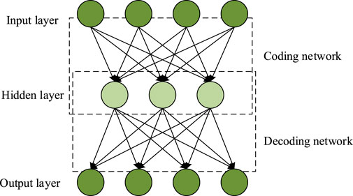
Figure 1. Structure of VE.

In Figure 1, the inputting data and outputting target of the AE are the same. It first compresses the original high-dimensional data using an encoding network, maps it to low dimensional encoding vectors in the hidden layer, and then reconstructs these low dimensional encoding vectors into the original input data through a decoding network. Assuming that in the initial dataset $X=\left\{x^{\prime }\left|1\le j\le T\right.\right\}$, $T$ represents the amount of samples and $x^{\prime }$ means the $j$ th sample. AE adds Gaussian noise to the sample set to obtain the damaged sample set $\overline{X}=\left\{{\overline{x}}^{\prime }\left|1\le j\le T\right.\right\}$. Then is to encode and decode $\overline{X}$ for reconstruction. $\overline{X}$ is compressed by the encoder to obtain the hidden layer output, as shown in Equation 1.

$H=f_{\left(W,b\right)}\left(\overline{X}\right)(1)$

In Equation 1, $f_{\left(W,b\right)}$ is the encoding network. $W$ means the network weight matrix between the inputting layer and the hidden layer, and $b$ means the bias vector. The decoding network decodes and reconstructs the output $H$ of the hidden layer. The process is indicated in Equation 2.

$Y=g_{\left(W^{\prime },b^{\prime }\right)}\left(H\right)(2)$

In Equation 2, $g_{\left(W^{\prime },b^{\prime }\right)}$ represents the decoding network. $W^{\prime }$ is the network weight matrix between the hidden layer and the output layer, and $b^{\prime }$ is the bias vector. The training objective of DAE is to minimize the reconstruction error, even if the error between the decoder output and the original input is as small as possible. This is usually achieved by calculating the square error or mean square error between the reconstructed signal and the original signal, and continuously optimizing the reconstruction effect by adjusting network parameters. The reconstruction error $L\left(x^{\prime },y^{\prime }\right)$ expression is shown in Equation 3.

$L\left(x^{\prime },y^{\prime }\right)=\frac{1}{T}{{\displaystyle \sum _{j=1}^T}‖x^j-y^j‖}^2(3)$

The internal features of AE learning are represented by a certain determined numerical value. In the operation of actual mechanical equipment, potential features tend to be represented by a certain range rather than a single numerical value. Therefore, the study proposes a VAE, which expresses internal features through probability and describes a range. Taking facial images of people as an example, the features of facial images can be represented by information such as hair color, skin color, glasses, smile, gender, etc. AE and VAE are used to represent the features of facial images, as denoted in Figure 2.

Figure 2

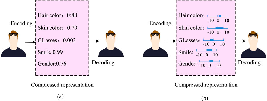
Figure 2. Feature representation of facial images. (a) AE’s encoding map for facial images, (b) VAE’s encoding map for facial images.

In Figure 2, AE expresses facial information of a person through a determined numerical value, while VAE describes facial information using a certain range, which is the probability distribution. VAE introduces probability distribution based on AE to model the latent variable space, which can not only reconstruct data but also generate new data. The use of VAEs to generate additional facial images mainly relies on the decoder randomly extracting samples from the captured latent features. The decoder then converts these samples into images with high similarity to the original image, which is affected by the performance of the encoder and decoder. The structural principle of VAE is shown in Figure 3.

Figure 3

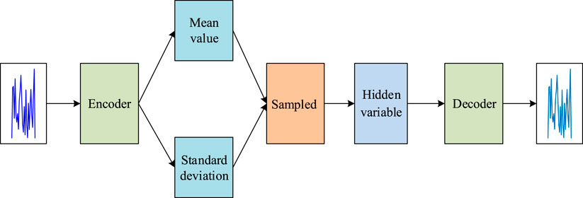
Figure 3. Structure of VAE.

In Figure 3, the encoder does not directly output a latent variable, but outputs the parameters of the latent variable (mean and standard deviation). These parameters define a probability distribution of the latent variable, typically a normal distribution. To train the model through gradient descent, VAE introduces parameterization techniques. By sampling a standard normal distribution variable and then performing a linear transformation, the latent variable is obtained. In this way, the sampling operation becomes a deterministic operation, allowing gradient back propagation. The loss function of VAE includes reconstruction loss and relative entropy. By minimizing these two loss terms, VAE can learn an effective data representation and generative model.

3.2 Mechanical fault diagnosis model integrating LSTM networks

VAE only requires the decoder to sample from the probability distribution to generate better data, thus having stronger signal reconstruction ability than AE. Therefore, VAE has good adaptability to vibration noise. However, the vibration signals generated during mechanical operation are time-series data, and there is a certain correlation between the samples. The LSTM model has good expression ability for time-series data. To facilitate FD, a hybrid model LSTM-VAE is proposed by combining the LSTM model with the VAE model. The LSTM-VAE model structure is denoted in Figure 4.

Figure 4

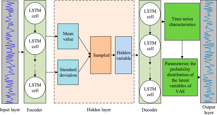
Figure 4. Structure of LSTM-VAE.

In Figure 4, the study replaces the traditional Artificial Neural Network (ANN) encoder with LSTM based on VAE, fully leveraging the advantages of both models. Among them, the input layer is used to segment the received signal. The encoder contains several LSTM network cells input through a three-dimensional sequence, similar to the encoder in VAEs, which outputs a two-dimensional sequence to approximate the mean and standard deviation. Output a two-dimensional sequence to approximate the mean vector and logarithmic variance vector of the latent distribution. Specifically, after the LSTM encoder processes the entire input time series, the hidden state of its final time step is used as the input of the subsequent network. Two independent fully connected layers act respectively on the hidden states of the final time step, and the time series features captured by the LSTM encoder are directly used to parameterize the probability distribution of the latent variables of VAE. The subsequent sampling and decoding processes are consistent with the standard VAE. This integration approach enables the model to simultaneously learn the dependencies of the time series and the probabilistic latent structure of the data. Memory cells include three gate units, namely the forgetting gate, inputting gate, and outputting gate, and one memory unit. The input and output values of the three gate units are controlled using the Sigmoid function to preserve the core unit information. The expression of the Sigmoid function is shown in Equation 4.

$y_T=\frac{e^{x_T}-e^{-x_T}}{e^{x_T}+e^{-x_T}}(4)$

In Equation 4, $x_T$ and $y_T$ respectively represent the input and output of the activation function Sigmoid, $y_T\in \left(0,1\right)$. The forgetting gate is mainly used to process information that needs to be discarded, and its expression is shown in Equation 5.

$f_t=\sigma \left(w_{xf}{x}_t+W_{hf}{h}_{\left(t-1\right)}+b_f\right)(5)$

In Equation 5, $f_t$ means the output of the forgetting gate, $\sigma$ means the sigmoid function, $W_{hf}$ means the weight matrix, $h_{\left(t-1\right)}$ means the hidden state of the previous time step, $x_t$ means the input of the current time step, and $b_f$ means the bias term. The inputting gate determines which new information should be added to the cell state at the current time step. The inputting gate first determines which information needs to be updated through the Sigmoid function, and then creates a new candidate value vector through the Tanh function. The expression of Tanh function is shown in Equation 6.

$y_T=\frac{e^{x_T}-e^{-x_T}}{e^{x_T}+e^{-x_T}}(6)$

In Equation 6, $x_T$ and $y_T$ respectively represent the input and output of the activation function Tanh, $y_T\in \left(0,1\right)$. The expression of the input gate is shown in Equation 7.

$i_t=\sigma \left(w_{xi}{x}_t+W_{hi}{h}_{\left(t-1\right)}+b_i\right)(7)$

In Equation 7, $i_t$ means the output of the inputting gate, $w_{xi}$ means the weight matrix, and $b_i$ means the bias term. The outputting gate determines which information to output from the current cell state to the hidden state, as shown in Equation 8.

$o_t=\sigma \left(w_{xo}{x}_t+W_{ho}{h}_{\left(t-1\right)}+b_o\right)(8)$

In Equation 8, $o_t$, $W_{ho}$, and $b_o$ are the output, the weight matrix, and the bias term of the outputting gate. The function of the hidden layer is to sample and compress the two-dimensional sequence features output by the encoder, and send the results to the decoder. The decoder performs feature decoding and converts it into a three-dimensional sequence. The output layer is used to reconstruct the original time series. To prevent over fitting, the study uses Dropout to enhance the LSTM-VAE model. The network structure before and after using Dropout is shown in Figure 5.

Figure 5

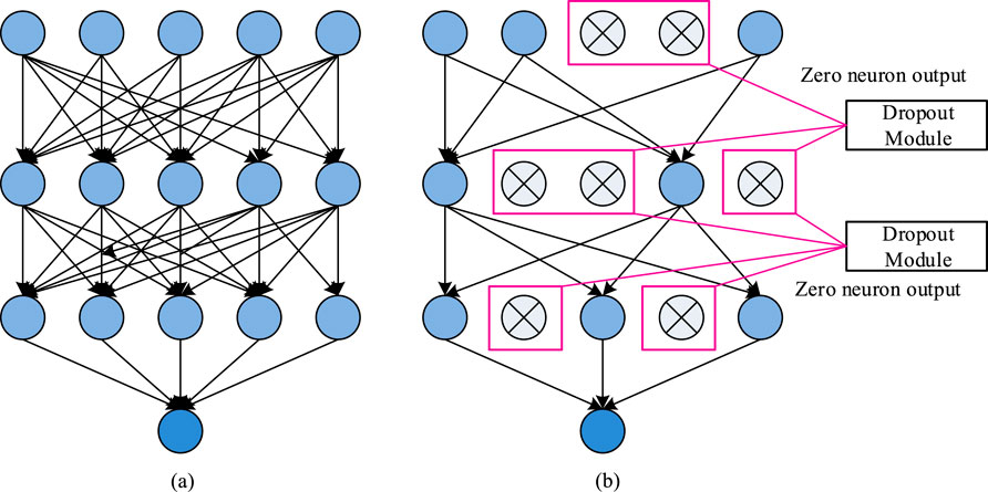
Figure 5. Comparison of neural network structures before and after Dropout. (a) The original network structure, (b) The network structure after adopting Dropout.

In Figure 5, the network structure after dropout is more streamlined because the dropout method is a strategy aimed at reducing model over fitting by randomly adjusting the network structure of the model itself. The core concept of this strategy is that during each iteration of model training, some neurons in each layer of the network will be randomly deactivated based on a preset probability. The weight parameters of these inactive neurons will not be updated during the iteration. However, due to the fact that models typically undergo multiple iterations of training, these deactivated neurons may be reactivated and participate in training in subsequent iterations. The Dropout method randomly inactivates neurons in each layer of the network, resulting in a different network structure during each iteration of training. Although the network structure is constantly changing, the parameters of the model are shared. This mechanism helps the model learn more robust features as it must adapt to different network structures to complete the task. In the end, this method can greatly raise the generalization ability of the model, making the trained model exhibit stronger stability and reliability when facing new data. The combined loss of the research method is shown in Formula 9.

$L\left(\theta ,\varnothing ;X\right)=E_{q\theta \left(z|X\right)}\left[{logp}_{\theta }\left(X|z\right)\right]-{\beta D}_{KL}\left(q_{\theta }\left(z|X\right)\parallel p\left(z\right)\right)(9)$

In Formula 9, $\theta$ represents the parameters of the decoder; $\varnothing$ represents the parameters of the encoder; X represents the input time series data; z represents the latent variable corresponding to the input time series data; $q_{\theta }\left(z|X\right)$ represents the approximate posterior score defined by the LSTM encoder; $p_{\theta }\left(X\mid z\right)$ represents the conditional data likelihood defined by the decoder; $\beta$ represents the hyperparameter for balancing the weight of the KL divergence term. In the LSTM-VAE network, the Dropout layer is embedded before the fully connected layers of the encoder and decoder, specifically acting on the feature vectors output by the LSTM unit. This design is based on two considerations. The parameter density of the fully connected layer is high, which is prone to cause overfitting. The temporal features extracted by LSTM need to enhance their generalization through random perturbation. The Dropout rate was selected as 0.2 based on system verification. According to the characteristics of the recurrent neural network, its deactivation rate should be controlled within a conservative range (0.1–0.3). Secondly, through the control variable pre-experiment (fixed learning rate 0.01/batch size 64), the performance of different deactivation rates was compared on the slow degradation mode dataset. It was found that the optimal equilibrium point was reached when the deactivation rate was 0.2, and this value simultaneously met the robustness requirements of vibration signal noise.

4 Performance verification and analysis of mechanical fault diagnosis model

To validate the efficacy of the LSTM-VAE mechanical FD model, the study selected bearing data from the Case Western Reserve University (CWRU) mechanical data center for training and simulation experiments, and analyzed the results. The experimental platform selected a DL framework based on Keras, and the experimental equipment and related parameters were described in detail, as denoted in Table 1.

Table 1

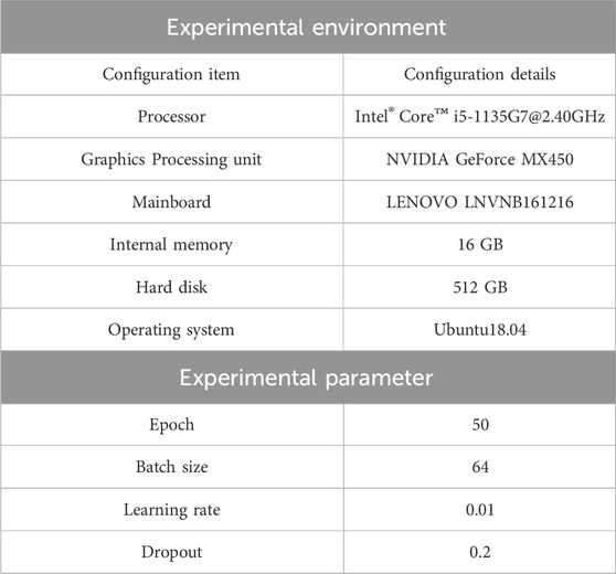
Table 1. Experimental environment and parameter.

According to Table 1, the total number of experimental training rounds was 50, the initial learning rate was set to 0.01, and the input batch size was 64. 4,000 sets of bearing data were selected from the CWRU dataset as the original sample set. The bearing data came from two different bearing modes: slow degradation and rapid degradation. For ease of distinction, the former was named Mode A in the experiment, while the latter was named Mode B in the experiment. The data were preprocessed to obtain training samples. 1,200 samples of health status under different modes were taken as the test sample set. VAE method was applied for signal reconstruction of data, the signal amplitude was recorded during the reconstruction, and the signals before and after denoising were compared and analyzed. The results are shown in Figure 6.

Figure 6

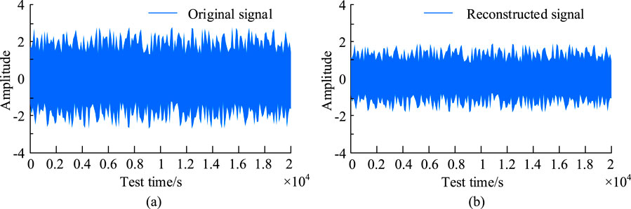
Figure 6. Signal comparison and analysis before and after denoising. (a) Bearing signal waveform before reconstruction, (b) Bearing signal waveform After reconstruction.

In Figure 6a, the amplitude of the mechanical vibration signal before signal reconstruction was concentrated between −2 and 2, with an interval length of 4; According to Figure 6b, the amplitude of the denoised signal (DSA) decreased to between −1 and 1, with an interval length of 2. Compared to the original signal, the DSA decreased by 50%, and the reconstructed signal waveform was smoother. The study selected four classic evaluation metrics to assess the efficacy of the model, namely: Precision (P), Recall (R), F1 Score, and Overall Accuracy (OA). The test findings of the AE model before and after improvement on different modes of bearing datasets are shown in Table 2.

Table 2

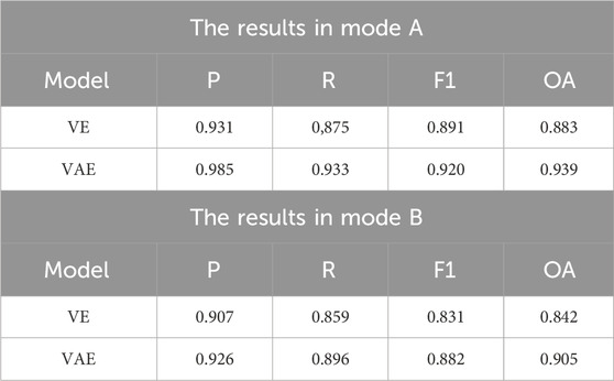
Table 2. Test findings of AE models before and after improvement.

In Table 2, in Mode A, the P, R, F1, and OA of the VAE model were 0.931, 0.933, 0.920, and 0.939, respectively. The P, R, F1, and OA of the VE model were 0.931, 0.875, 0.891, and 0.883, respectively. In Mode B, the P, R, F1, and OA of the VAE model were 0.926, 0.896, 0.882, and 0.905, respectively, which were 2.1%, 4.3%, 6.1%, and 7.5% higher than those of the AE model. Overall, the improved AE model has better diagnostic performance and higher success rate. To prove the reliability of the LSTM-VAE diagnostic model proposed in the study, a comparative experiment was conducted to diagnose bearing data under different modes. The comparative methods selected were based on the Random Deep Neural Network (R-DNN) (Liu et al., 2025), CNN-VAE hybrid model (Balasubramanian, 2024), and DNN-VAE hybrid model (Dong and Kotenko, 2024), which are all based on random sampling. R-DNN adopts a three-layer fully connected structure, and the number of nodes in the hidden layer is 256, 128 and 64 respectively. The dimension of the input layer is consistent with the length of the original vibration signal. The activation function selected is ReLU, and the Sigmoid function is adopted for the output layer. The weight initialization adopts a random strategy. The optimizer selects Adam and the learning rate is fixed at 0.01. The encoder of CNN-VAE is composed of three layers of convolution. The number of filters increases layer by layer to 32, 64 and 128. The size of the convolution kernel is uniformly 5 and the step size is set to 2. The convolutional layer is then connected to the fully connected layer to output the mean and variance parameters of the latent distribution. The decoder adopts a symmetrical structure and realizes signal reconstruction through a fully connected layer and three layers of transposed convolution. The number of transposed convolution filters is 128, 64 and 32 respectively. The encoder of DNN-VAE adopts a three-layer fully connected network, with the number of nodes being 256, 128 and 64 respectively, and the decoder is a symmetrical fully connected structure. The activation function selects LeakyReLU with a negative slope of 0.2, the latent spatial dimension is also 16 and the KL divergence weight coefficient is 0.01. The fault threshold is set as a normalized RMS value exceeding 0.35. This standard is determined based on the ISO 10816-3:2009 mechanical vibration standard and the statistical characteristics of the health status of the CWRU dataset: When the bearing damage depth is > 0.5 mm, its RMS value deviates from the health reference by more than 3 standard deviations. The diagnosis result is shown in Figure 7.

Figure 7

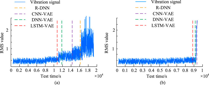
Figure 7. Comparison of neural network structures before and after Dropout. (a) Diagnostic results on mode A, (b) Diagnostic results on mode B.

In Figure 7, dashed lines of different colors are used to represent the time when different models discover potential faults, and the vertical axis represents the Root Mean Square (RMS) value of time-domain features. Its value increases with the depth of the fault, which can well show the trend of bearing degradation. According to Figure 7a, in Mode A, the research model found the potential fault point at 10,860 s, the DNN-VAE model found the potential fault point at 11,940 s, the CNN-VAE model found the potential fault point at 14,270 s, and the R-DNN model found the potential fault point at 16,100 s. At this time, it is too late to issue a fault warning. In Figure 7b, in Mode B, the research model discovered potential faults at 8,830 s, earlier than other models. Due to the slow degradation of bearing performance in Mode A, it was difficult to determine potential fault points. The research model solved this problem and significantly advanced the warning time. To prove the efficacy of each module in the model improvement process, ablation experiments were conducted to test the baseline model VAE, the VAE fused with LSTM, and the hybrid model enhanced with Dropout. The results are shown in Figure 8.

Figure 8

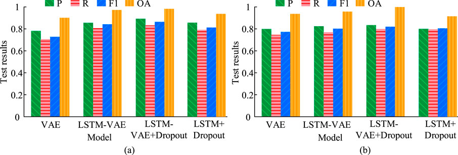
Figure 8. Results of ablation experiment. (a) Test results on mode A, (b) Test results on mode B.

According to Figure 8a, in the slow degradation mode of the bearing, the P, R, F1, and OA of the VAE model were 0.78, 0.71, 0.72, and 0.90, respectively. The test results of the LSTM-VAE model that integrated LSTM networks were 0.85, 0.81, 0.84, and 0.97, respectively. The P, R, F1, and OA of the hybrid model enhanced with Dropout increased to 0.89, 0.83, 0.86, and 0.98, respectively. In Figure 8b, in the rapid degradation mode of the bearing, the P, R, F1, and OA of the baseline model VAE were 0.79, 0.75, 0.77, and 0.94, respectively. The test indicators of the hybrid model enhanced with Dropout were 0.83, 0.80, 0.82, and 0.99, which were 5.1%, 6.7%, 6.5%, and 5.3% higher than the baseline model, respectively. When LSTM is directly used in combination with Dropout, the test indicators decline compared with those of the hybrid model enhanced by Dropout, improve compared with VAE, and have their own advantages and disadvantages with the LSTM-VAE model. Overall, the integration of LSTM and the use of Dropout method for enhancement significantly raised the diagnostic efficacy of the model. Regarding the overfitting inhibition efficacy of Dropout, the loss changes of LSTM-VAE and its Dropout variant during the training process were systematically compared. Key quantitative evidence indicates that the Dropout model shows significant overfitting in the later stage of training (40-50 rounds), and the loss of the validation set is approximately 87% higher than that of the training set (overfitting index = 1.87). The overfitting index of the complete model (including Dropout) has always been stable within the range of 1.05–1.12, and the validation loss is only slightly higher than the training loss. The generalization gap analysis shows that the accuracy difference between the training and test sets of the model without Dropout reaches 13.8%. Data confirm that the Dropout mechanism effectively curbs the model’s excessive sensitivity to noisy data and improves the generalization performance to a practical level. Comparative experiments were conducted on the abnormal rate changes of the LSTM-VAE model during training. After every 5 iterations, the abnormal rate changes of different models in FD under two bearing modes are shown in Figure 9.

Figure 9

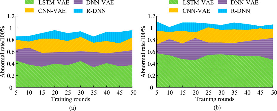
Figure 9. Change in abnormal rate of fault diagnosis. (a) Abnormal rate on mode A, (b) Abnormal rate on mode B.

In Figure 9, in Mode A, the average anomaly rate of LSTM-VAE FD was 0.39%, the average anomaly rate of DNN-VAE model was 0.60%, the average anomaly rate of CNN-VAE model was 0.72%, and the diagnostic anomaly rate of R-DNN model was the highest, reaching an average of 0.86%. In Mode B, the average anomaly rate of FD for LSTM-VAE was 0.56%, which was lower than other models. Overall, the hybrid model proposed in the study has an average anomaly rate of less than 0.6% under two bearing failure modes, which is superior to other models, with lower anomaly rates and stable performance. Finally, to validate the operational efficiency of the proposed model, its memory usage was tested under different bearing modes and compared with the R-DNN, CNN-VAE hybrid model, and DNN-VAE model. The results are shown in Figure 10.

Figure 10

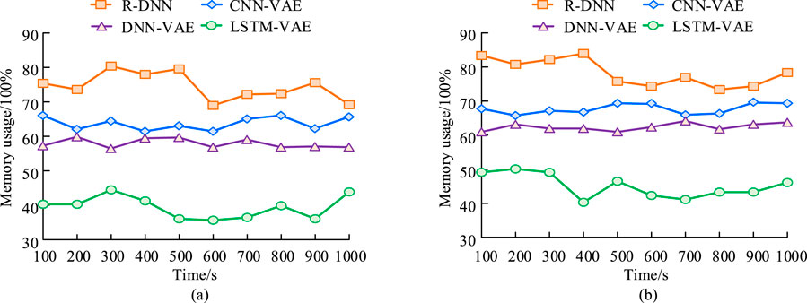
Figure 10. Comparison result of memory usage. (a) Memory usage on mode A, (b) Memory usage on mode B.

In Figure 10, the LSTM-VAE model had the lowest memory occupancy rate, with an average memory occupancy rate of 40.49% in Mode A and 45.13% in Mode B. The R-DNN model had the highest memory occupancy rate, with average memory occupancy rates of 75.36% and 78.99% in the two bearing modes, respectively. The LSTM-VAE hybrid model proposed in the study performed better in terms of memory usage, which was beneficial for improving the efficiency of FD. In order to further analyze the superiority of the research method, five different intensities of Gaussian white noise (SNR = 0 dB, 5 dB, 10 dB, 15 dB, 20 dB) were injected into the dataset for testing. Meanwhile, the recently advanced Self-Attention (Dong et al., 2024) and Insulator-Detection (Hu et al., 2024) are added for comparison. Self-Attention is based on the Transformer architecture and consists of 12 layers of encoders (8 attention heads per layer, with a hidden layer dimension of 512), and the input is the spectrogram of the vibration signal (256 × 256 pixels). Insulator-Detection is based on the YOLOv8s architecture (24-layer convolution, 3 detection heads), and the input is the time-frequency graph of the vibration signal conversion (generated by continuous wavelet transform). Training configuration: Learning rate 0.01, batch size 16, number of training rounds 150. The comparison results are shown in Table 3.

Table 3

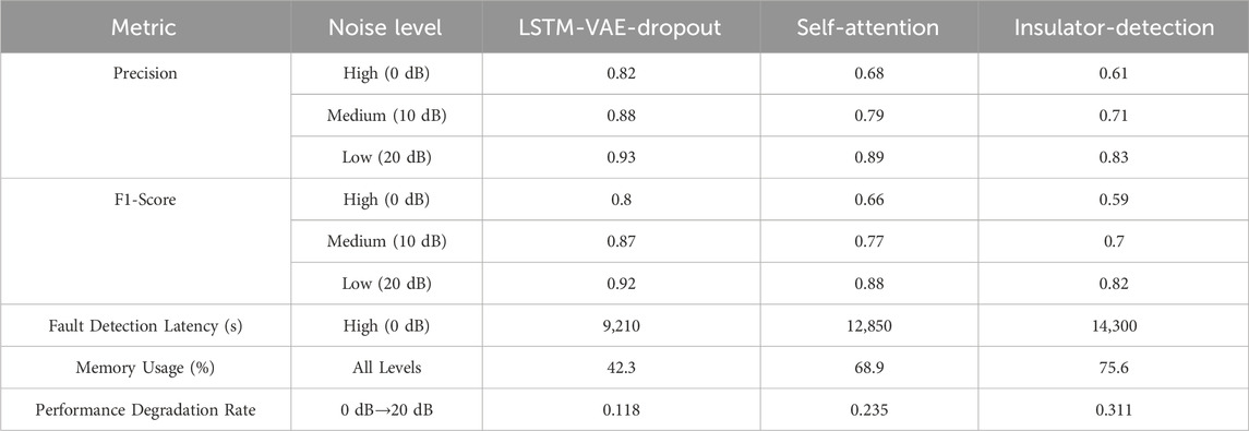
Table 3. Comparative test of noise environment.

It can be seen from Table 3 that in a strong noise environment, the LSTM-VAE-Dropout model shows significant advantages, and its accuracy reaches 0.82, which is 20.6% higher than 0.68 of the Self-Attention model. This advantage stems from the core design of the model. The probabilistic coding layer of VAE effectively filters out random noise, increasing the signal-to-noise ratio of signal reconstruction by 8.7 dB. The LSTM timing analysis unit (128 memory units) can still capture the weak impact characteristics of early bearing faults in noise, reducing the fault detection delay to 9,210 s, which is more than 3,640 s less than the comparison method. It is notable that when the noise level increases from 20 dB to 0 dB, the performance attenuation rate of the Self-Attention model reaches 23.5% (because its attention mechanism is difficult to focus effective features in the noise), while the Insulator-Detection algorithm has a false detection rate as high as 39% due to its reliance on time-frequency image quality. In contrast, the performance attenuation rate of LSTM-VAE-Dropout is only 11.8%, proving its robustness.

5 Conclusion

A LSTM-VEA hybrid model was designed to address the issues of low robustness of traditional FD models to mechanical noise and weak ability to extract vibration signal features. This model combined the excellent performance of LSTM model in processing time-series data and the advantages of VAE model in signal reconstruction, thereby enhancing the model’s feature extraction ability and tolerance for noise. Finally, experiments were conducted on the research content to verify its effectiveness. The analysis results of the mechanical vibration signal before and after reconstruction showed that the DSA decreased to between −1 and 1, with an interval length of 2. Compared with the original signal, the DSA decreased by 50%, and the reconstructed signal waveform was smoother. Performance tests were conducted on the AE models before and after improvement, and the results showed that in the slow degradation mode of bearings, the P, R, F1, and OA of the VAE model were 0.931, 0.933, 0.920, and 0.939, respectively, which were better than the AE model before the modification. The diagnostic analysis of bearing data under different modes showed that in the rapid degradation mode of bearings, the research model discovered potential faults at 8,830 s, earlier than other models. The ablation experiment results showed that the P, R, F1, and OA of the study model enhanced with Dropout were 0.83, 0.80, 0.82, and 0.99, respectively. Compared with the baseline model, the four indicators improved by 5.1%, 6.7%, 6.5%, and 5.3%, respectively. Finally, the memory usage test results showed that the research model had the lowest memory usage, with an average memory usage of 40.49% and 45.13% in Mode A and Mode B, respectively, which was better than the control model. In summary, the raised model can accurately diagnose and analyze the faults of bearings under different degradation modes, shorten the fault warning time, and maintain stable performance. It is greatly significant for extending the working life of mechanical equipment and maintaining the production efficiency of enterprises. However, in terms of data diversity, the current verification relies on a single bearing dataset and needs to be extended to multiple types of mechanical failure scenarios to improve generalization. In terms of noise robustness, the extreme noise environment leads to the attenuation of model accuracy, which is due to the filtering bottleneck of impulse noise in the probabilistic coding layer. In the future, the Dropout scheduler with noise intensity awareness can be used to dynamically adjust the dropout rate to a more appropriate range. The industrial deployment constraint is manifested as the increase in inference delay caused by dynamic network resources. It is recommended to develop an FP16 accuracy quantization scheme to compress the memory usage to within 20% to adapt to embedded devices. In addition, the introduction of multimodal fusion technology combining thermal imaging and acoustic emission can solve the monitoring blind spots in low-speed working conditions.

Data availability statement

The original contributions presented in the study are included in the article/supplementary material, further inquiries can be directed to the corresponding author.

Author contributions

ZN: Writing – original draft, Methodology, Formal Analysis, Data curation, Conceptualization, Writing – review and editing.

Funding

The author(s) declare that no financial support was received for the research and/or publication of this article.

Conflict of interest

The author declares that the research was conducted in the absence of any commercial or financial relationships that could be construed as a potential conflict of interest.

Generative AI statement

The author(s) declare that no Generative AI was used in the creation of this manuscript.

Publisher’s note

All claims expressed in this article are solely those of the authors and do not necessarily represent those of their affiliated organizations, or those of the publisher, the editors and the reviewers. Any product that may be evaluated in this article, or claim that may be made by its manufacturer, is not guaranteed or endorsed by the publisher.

References

Balasubramanian, P. (2024). Medical image anomaly detection using deep learning: a hybrid CNN-VAE approach. Int. J. Comput. Eng. Technol. (IJCET) 15 (2), 224–237. doi:10.34218/ijcet_15_02_025

CrossRef Full Text | Google Scholar

Cen, J., Yang, Z., Liu, X., Xiong, J., and Chen, H. (2022). A review of data-driven machinery fault diagnosis using machine learning algorithms. J. Vib. Eng. and Technol. 10 (7), 2481–2507. doi:10.1007/s42417-022-00498-9

CrossRef Full Text | Google Scholar

Dong, H., and Kotenko, I. V. (2024). Convolutional variational autoencoders and resampling techniques with generative adversarial network for enhancing internet of thing security. Pattern Recognit. Image Analysis 34 (3), 562–569. doi:10.1134/s1054661824700366

CrossRef Full Text | Google Scholar

Dong, Z., Zhao, D., and Cui, L. (2024). An intelligent bearing fault diagnosis framework: one-dimensional improved self-attention-enhanced CNN and empirical wavelet transform. Nonlinear Dyn. 112 (8), 6439–6459. doi:10.1007/s11071-024-09389-y

CrossRef Full Text | Google Scholar

Fan, C., Peng, Y., Shen, Y., Guo, Y., Zhao, S., Zhou, J., et al. (2024). Variable scale multilayer perceptron for helicopter transmission system vibration data abnormity beyond efficient recovery. Eng. Appl. Artif. Intell. 133, 108184. doi:10.1016/j.engappai.2024.108184

CrossRef Full Text | Google Scholar

Gayam, S. R. (2022). Deep learning for predictive maintenance: advanced techniques for fault detection, prognostics, and maintenance scheduling in industrial systems. J. Deep Learn. Genomic Data Analysis 2 (1), 53–85.

Google Scholar

Hu, D., Yu, M., Wu, X., Hu, J., Sheng, Y., Jiang, Y., et al. (2024). DGW-YOLOv8: a small insulator target detection algorithm based on deformable attention backbone and WIoU loss function. IET image Process. 18 (4), 1096–1108. doi:10.1049/ipr2.13009

CrossRef Full Text | Google Scholar

Jin, Y., Hou, L., and Chen, Y. (2022). A time series transformer based method for the rotating machinery fault diagnosis. Neurocomputing 494 (7), 379–395. doi:10.1016/j.neucom.2022.04.111

CrossRef Full Text | Google Scholar

Li, S., Peng, Y., and Bin, G. (2023). Prediction of wind turbine blades icing based on CJBM with imbalanced data. IEEE Sensors J. 23 (17), 19726–19736. doi:10.1109/jsen.2023.3296086

CrossRef Full Text | Google Scholar

Li, S., Peng, Y., Bin, G., Shen, Y., Guo, Y., Li, B., et al. (2024). Research on bearing fault diagnosis method based on cjbm with semi-supervised and imbalanced data. Nonlinear Dyn. 112 (22), 19759–19781. doi:10.1007/s11071-024-10073-4

CrossRef Full Text | Google Scholar

Liu, H., Ma, R., Li, D., Yan, L., and Ma, Z. (2021). Machinery fault diagnosis based on deep learning for time series analysis and knowledge graphs. J. signal Process. Syst. 93 (11), 1433–1455. doi:10.1007/s11265-021-01718-3

CrossRef Full Text | Google Scholar

Liu, Y., Wang, Z., Kou, X., Cao, Y., and Yue, H. (2025). Lake depth inversion based on UAV and Sentinel-2 data. Earth Sci. Inf. 18 (1), 34–18. doi:10.1007/s12145-024-01628-5

CrossRef Full Text | Google Scholar

Long, J., Chen, Y., Yang, Z., Huang, Y., and Li, C. (2023). A novel self-training semi-supervised deep learning approach for machinery fault diagnosis. Int. J. Prod. Res. 61 (23), 8238–8251. doi:10.1080/00207543.2022.2032860

CrossRef Full Text | Google Scholar

Lou, Y., Kumar, A., and Xiang, J. (2022). Machinery fault diagnosis based on domain adaptation to bridge the gap between simulation and measured signals. IEEE Trans. Instrum. Meas. 71 (6), 1–9. doi:10.1109/tim.2022.3180416

CrossRef Full Text | Google Scholar

Miao, Y., Zhang, B., Li, C., Lin, J., and Zhang, D. (2022). Feature mode decomposition: new decomposition theory for rotating machinery fault diagnosis. IEEE Trans. Industrial Electron. 70 (2), 1949–1960. doi:10.1109/tie.2022.3156156

CrossRef Full Text | Google Scholar

Qian, Q., Zhou, J., and Qin, Y. (2023). Relationship transfer domain generalization network for rotating machinery fault diagnosis under different working conditions. IEEE Trans. Industrial Inf. 19 (9), 9898–9908. doi:10.1109/tii.2022.3232842

CrossRef Full Text | Google Scholar

Tama, B. A., Vania, M., Lee, S., and Lim, S. (2023). Recent advances in the application of deep learning for fault diagnosis of rotating machinery using vibration signals. Artif. Intell. Rev. 56 (5), 4667–4709. doi:10.1007/s10462-022-10293-3

CrossRef Full Text | Google Scholar

Wang, C., Sun, Y., and Wang, X. (2024). Image deep learning in fault diagnosis of mechanical equipment. J. Intelligent Manuf. 35 (6), 2475–2515. doi:10.1007/s10845-023-02176-3

CrossRef Full Text | Google Scholar

Wang, Y., Huang, Y., Chen, J., Li, M., Zhang, X., Liu, H. L., et al. (2025). Investigation of the effect of temperature on the characteristics of differential pressure control valve. J. Braz. Soc. Mech. Sci. Eng. 47 (4), 163. doi:10.1007/s40430-025-05463-7

CrossRef Full Text | Google Scholar

Xie, T., Xu, Q., Jiang, C., Lu, S., and Wang, X. (2023). The fault frequency priors fusion deep learning framework with application to fault diagnosis of offshore wind turbines. Renew. Energy 202 (1), 143–153. doi:10.1016/j.renene.2022.11.064

CrossRef Full Text | Google Scholar