Multiscale electromagnetic–thermal–fluid field coupling model for oil-immersed transformers

Accurate predictions of the hotspot temperatures within large oil-immersed transformers are critical to their operational safety and longevity. The present work explores a novel multiscale electromagnetic–thermal–fluid indirect coupling model to address this challenge. The novelty of the model lies in its comprehensive integration of a detailed disc-type winding structure with the complete radiator-cooling circuit to overcome the common simplifications applied in existing studies. The proposed methodology involves a sequential process, where a 3D electromagnetic field simulation is first performed to determine the loss distribution precisely; here, the total eddy current loss of the winding accounts for 3.68% of the total winding loss and shows a U-shaped distribution in the winding disc height direction. These losses are then imported as heat sources into a full-scale thermal–fluid model. The key findings of the model are that the eddy current losses of the winding account for a significant portion of the total loss and that their distribution critically influences the temperature field; further, the presence of oil washers creates localized temperature differences of up to 5.3 K. The model accuracy is strongly validated through a transformer temperature rise test using embedded optical-fiber sensors, and the results show a maximum deviation of only 3.1 K. Hence, the present study provides a high-fidelity simulation framework for transformer thermal management and design optimization.

1 Introduction

The internal insulation problem of a transformer is one of the main reasons for transformer outages (CIGRE Working Group A2.37, 2015). The hotspot temperature (HST) of a transformer winding significantly impacts the oil paper insulation aging rate, where a high winding HST can cause bubble generation leading to failure of the insulation materials (Hill et al., 2019). However, the HST of a transformer winding is typically measured inside the transformer and is difficult to obtain directly. To obtain the accurate value of the winding HST, we must fully understand the heat generation and dissipation processes of the transformer as a whole, identify multiple characteristics reflecting the transformer thermal state, and build a model or method to effectively detect the winding HST.

The digital twin technology integrates physical and data-driven models, including the physical model of the equipment, real-time sensor measurement data, and historical data during equipment operation, to virtually map the equipment entity in the virtual space as well as realize real-time perception of the operational state of the actual physical system (Li et al., 2022; Yang et al., 2025). Transformer digital twin technologies have been preliminarily explored and applied in the real-time detection of transformer internal faults (Hamidi, 2022), fault diagnosis and remaining life prediction of the transformer winding (Jing et al., 2022; Jing et al., 2021), monitoring of transformer medium voltage based on low-voltage (LV) measurements (Moutis and Alizadeh-Mousavi, 2021), and estimation of transformer on-load tap changer condition (Kim et al., 2022). The transformer digital twin technology thus provides a technical approach to perceive the operation status accurately as well as propose efficient operating and maintenance strategies. The complete digital twin architecture mainly consists of five layers (Qi et al., 2021). Here, the high-fidelity multiphysics model serves as the foundational “physical model” within the model layer of the transformer digital twin system; its accuracy is a prerequisite for future real-time virtual sensing and predictive analytics. This model is a popular research topic for analyzing transformer heat dissipation characteristics with the multiphysical field calculation method.

Owing to the limitations of computing performance, calculations of the transformer thermal–fluid field are often restricted to analyses of important transformer components, such as the transformer windings and radiators. At the same time, these component structures are simplified during the simulations, such as ignoring the layered disc structure of the winding, establishing the windings as overall cylindrical structures, or changing the transformer winding model from three-dimensional to two-dimensional for the sake of analysis. Considering a typical transformer disc winding as the research object, Zhang et al. (2018) and Zhang et al. (2017) established a two-dimensional simulation model to analyze the oil flow distribution and pressure drop characteristics inside the winding, in addition to assessing the impacts of the winding structure, loss distribution, and ambient temperature on the transformer winding hotspot coefficient. Torriano et al. (2018) established a simplified model by considering the entire cooling circuit as well as the impact of the arrangement of different oil washers of the windings on the disc temperature and oil passage flow rate distribution in the windings. Dorella et al. (2024) performed computational fluid dynamics simulations to improve the heat dissipation in the power transformer radiator. Li et al. (2019) calculated the non-uniformly distributed power losses of a 2,500 kVA dry-type power transformer core and its foil windings; these losses were then applied to the 2D fluid model to obtain more accurate calculations of the winding temperature field results. Liu et al. (2022) applied optical-fiber temperature sensors to a 35 kV distribution transformer to monitor its windings and iron temperature distribution; they reported that the measured values were consistent with the results calculated using the finite element method.

To reduce the calculated values by accounting for radiators in the overall heat dissipation cycle of the transformer, some scholars have proposed indirect coupling analysis methods by establishing simplified models using radiators and coupling them with the thermal–fluid calculation model of the transformer tank and windings. Cheng et al. (2022) simplified the radiator-cooling duct to a one-dimensional model and combined it with the 3D model of the winding to construct a multiscale thermal–fluid calculation model for a 35 kV transformer. Stebel et al. (2022) proposed an electromagnetic–fluid–fluid indirect coupling thermal analysis model for an 8.5 MVA transformer and compared the cooling effects of esters and mineral oils. Notably, extant studies often have tradeoffs in multiphysical field calculations involving high-power transformers; these works have either modeled the global oil circulation using simplified winding structures or analyzed detailed winding models in isolation from the full radiator-cooling circuit.

In the present work, we propose a full electromagnetic–thermal–fluid indirect coupling analysis model to calculate the HST of the 50 MVA disk-type power transformer. Accordingly, we considered a refined disc-type winding structure and the influence of radiators on the overall oil circulation in the transformer to provide a computationally efficient and robust solution without significant loss of accuracy. The electromagnetic field of the transformer was also calculated to determine the loss distribution inside the transformer more accurately; then, using these losses as the heat sources, the thermal–fluid field of the transformer was solved by the finite volume method. The transformer temperature rise test was lastly conducted to verify the accuracy and effectiveness of the simulation analysis, where the three-phase windings were all embedded with optical-fiber temperature sensors.

2 Multiphysical field simulation analysis model

2.1 Electromagnetic field

The field quantities B and E can be expressed using the magnetic vector potential A and electric scalar potential φ (Fu et al., 2016):

$\mathit{B}=\nabla \times \mathit{A}=\mu \mathit{H},(1)$

$\mathit{E}=-\frac{\mathrm{\partial }\mathit{A}}{\mathrm{\partial }t}-\nabla \phi .(2)$

Here, B indicates the magnetic flux density (T), and H (A/m) and E (V/m) indicate the magnetic and electric field strengths, respectively.

As shown in Figure 1, by employing the Coulomb gauge condition, the complete descriptions of the electromagnetic field in the eddy current domain Ω₁ and source current domain Ω₂ can be expressed as follows:

$\left.\begin{array}{l}\nabla \times \left(\frac{1}{\mu }\nabla \times \mathit{A}\right)+\sigma \frac{\mathrm{\partial }\mathit{A}}{\mathrm{\partial }t}+\sigma \nabla \phi =0\\ \nabla ·\left(-\sigma \left(\frac{\mathrm{\partial }\mathit{A}}{\mathrm{\partial }t}+\nabla \phi \right)\right)=0\end{array}\right\}in{\mathrm{\Omega }}_1,(3)$

$\nabla \times \left(\frac{1}{\mu }\nabla \times \mathit{A}\right)=\mathit{J}in{\mathrm{\Omega }}_2,(4)$

Figure 1

Figure 1. Electromagnetic field regions based on the Coulomb gauge condition.

where σ indicates the electrical conductivity of the conductor (S/m) and J is the current density (A/m²).

2.2 Thermal–fluid field

2.2.1 Governing equations

In transformers that use oil for heat dissipation, the natural convection process of the oil helps realize heat transfer inside the transformer. The heat transfer process of the transformer oil flow can thus be analyzed by solving the Navier–Stokes equation.

This solution includes three basic differential equations of physics (Torriano et al., 2012), namely, the mass conservation, momentum conservation, and energy conservation equations:

Mass conservation equation:

$\frac{\mathrm{\partial }\rho }{\mathrm{\partial }t}+\nabla ·\left(\rho \mathit{v}\right)=0,(5)$

where ρ is the oil density (kg/m³) and v is the fluid velocity of the oil (m/s).

Momentum conservation equation:

$\frac{\mathrm{\partial }\left(\rho \mathit{v}\right)}{\mathrm{\partial }t}+\rho \mathit{v}·\nabla \mathit{v}=f-\nabla p+\eta {\nabla }^2\mathit{v},(6)$

where f is the unit oil mass force (N/m³), p is the oil pressure (Pa), and η is the dynamic viscosity (kg/(m·s)).

Energy conservation equation:

$\frac{\mathrm{\partial }\left(\rho c_{P}T\right)}{\mathrm{\partial }t}+\nabla ·\left(\rho c_{P}vT\right)=\nabla \left(k\nabla T\right)+S_E,(7)$

where k is the thermal conductivity (W/(m·K)), T is the temperature (K), c_p is the specific heat capacity of the oil (J/(kg·K)), and S_E is the heat-source term (W/m³).

To determine the solid-domain temperature distribution in the transformer, the solid-domain heat conduction is given as

$\frac{\mathrm{\partial }\left(\rho c_{P}T\right)}{\mathrm{\partial }t}=-\nabla \left(k\nabla T\right)+S_E.(8)$

For the incompressible transformer oil, the driving force of the oil caused by its density change is described using the Boussinesq approximation (Garelli et al., 2017):

$\rho ={\rho }_0\left(1-\beta ·\Delta T\right),(9)$

where ρ₀ indicates the oil density at the reference temperature T₀, ΔT indicates the oil temperature deviation from T₀, and β indicates the thermal expansion coefficient of the transformer oil.

2.2.2 Boundary conditions

In this work, the convection heat transfer coefficient h_c is used to express the heat transfer to the ambient (Lin et al., 2025); additionally, the heat flow q_r generated by the radiation heat transfer coefficient can be expressed as

$q_r=\epsilon ·{\sigma }_{\mathrm{b}}·\left(T_{\mathrm{W}}^4-T_{\mathrm{a}}^4\right),(10)$

where ε is the emissivity of the transformer outer shell surface, σ_b is the Stefan Boltzmann constant, T_w is the temperature of the transformer outer wall, and T_a is the ambient temperature.

The per-unit-area radiation heat transfer capacity of the transformer outer shell surface to the external environment can be considered to be equivalent to the radiation heat transfer coefficient h_r:

$h_r=\raisebox{1ex}{$q_r$}\!\left/ \!\raisebox{-1ex}{$\left(T_{\mathrm{W}}-T_{\mathrm{a}}\right)$}\right.=\epsilon ·{\sigma }_{\mathrm{b}}·\left(T_{\mathrm{W}}^2+T_{\mathrm{a}}^2\right)·\left(T_{\mathrm{W}}+T_{\mathrm{a}}\right).(11)$

2.3 Electromagnetic–thermal–fluid field indirect coupling method

In the coupling analysis of the electromagnetic–thermal–fluid field of the transformer, we considered the weak coupling relationship between the electromagnetic and thermal–fluid fields via an indirect coupling method. This indirect coupling procedure is outlined in Figure 2; accordingly, the electromagnetic field is considered as a form of heat source, and the transformer stray losses of the internal structural parts as well as iron shell and eddy current losses of the three-phase windings are calculated using electromagnetic field analysis before being loaded onto the thermal–fluid field simulation model.

Figure 2

Figure 2. Indirect coupling analysis of multiphysical fields.

3 Transformer temperature rise test

3.1 Temperature rise test transformer

As shown in Figure 3, the unit evaluated in this study is the SSZ11-50000/110 transformer operating under the “oil natural, air natural” cooling model; the rated capacity and rated voltage of the transformer are 50 MVA and 110 kV, respectively.

Figure 3

Figure 3. Physical structure of the transformer used in this study.

3.2 Optical-fiber temperature measurement system

Optical-fiber sensors are now widely used to monitor various transformer parameters, such as partial discharge, dissolved gases, and temperature (Ma et al., 2021). The fiber grating temperature sensor forms a spatial phase grating on the fiber core of the optical fiber upon ultraviolet exposure. The linear relationship between the wavelength drift of the reflected light and temperature is used to obtain temperature measurements. The optical fiber has good characteristics like high-temperature resistance, high-voltage (HV) resistance, and electromagnetic interference resistance. The performance and overall structure of the temperature sensor are shown in Table 1 and Figure 4, respectively. All sensors used in this study were calibrated against a precision reference thermometer in a controlled temperature bath prior to installation to ensure the stated accuracy of ±1 °C.

Table 1

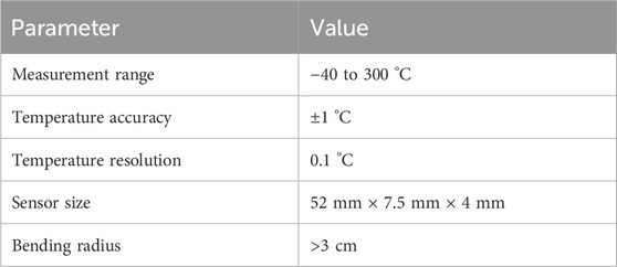
Table 1. Performance parameters of optical-fiber temperature sensors.

Figure 4

Figure 4. Optical-fiber temperature sensor used in this study.

The placement of the optical-fiber sensor was achieved by replacing the winding disc spacer in the original oil channel after embedding the sensor in the spacer. As shown in Figure 5, each phase winding has 20 spacer blocks about the circumference, the optical fibers are installed in the spacer blocks close to each other in the three-phase windings, and the winding optical-fiber temperature sensor in phase C is installed in the third spacer.

Figure 5

Figure 5. Diagram showing installation of the optical fiber in the oil duct.

In each phase, the HV, medium-voltage (MV), and LV windings are distributed in a cylindrical manner around the iron core. The HV and LV windings are divided into 86 discs each, while the MV winding is divided into 62 discs. As shown in Figure 6, internal oil washers are used to form the winding oil flow passes to promote horizontal oil duct flow velocity between the winding discs, which generates a zigzag oil flow.

Figure 6

Figure 6. Diagram showing installation of the optical fibers in the transformer windings.

The optical fiber is installed in the spacer block between the fourth and fifth discs counted from the top of each phase of the HV, MV, and LV windings. Here, three optical fibers are installed in each phase for a total of nine optical fibers. The schematic of the optical-fiber installation locations and photograph are shown in Figures 6, 7 respectively.

Figure 7

Figure 7. Optical-fiber temperature sensor installation in this study.

3.3 Temperature rise test results

When the transformer is in the rated HV and MV winding operation and voltage-regulating winding is in the most negative tapping condition, the transformer no-load and load test results show a no-load loss of 35.29 kW and load loss of 260.4 kW. The short-circuit method recommended in the testing standard is used to conduct the temperature rise test (Power transformers, 2011). During the temperature rise test, the MV windings are shorted and HV windings are connected to the voltage-regulating power supply. The process of the temperature rise test comprises two stages. The first stage is the total loss stage, where the sum of the transformer no-load and load losses is applied to the HV and MV windings. When the change in temperature rise at the monitoring point is less than 1 K/h and has been maintained for 3 h, the test enters the second temperature rise stage. In the second stage, only the transformer load loss is applied to the HV and MV windings, and this stage lasts approximately 0.5 h.

Figure 8 shows the transformer temperature rise test platform used in this study. The internal and external optical fibers are connected through the optical-fiber cable flange plate, and the temperature information is transmitted to the acquisition software on the computer through the optical-fiber signal demodulator for data storage and analysis. The temperature rise results at the designated monitoring points on the HV and MV windings are shown in Figure 9.

Figure 8

Figure 8. Transformer temperature rise test platform used in this study.

Figure 9

Figure 9. Temperature rise test results for different windings and phases.

4 Results and discussion

4.1 Transformer magnetic field simulation and analysis

4.1.1 Calculation model

The heat radiators in the transformer are distributed along the iron shell; given the good magnetic conductivity of the shell, the magnetic line of force passing through the radiators is greatly limited. Therefore, when establishing the transformer magnetic field calculation model, the radiators, bushings, and stiffening plates on the shell are removed. The magnetic field calculation model for the 110 kV transformer, including the magnetic shielding structure of the shell, upper and lower clamps, and tie plate of the core, is shown in Figure 10. An air layer is also established around the transformer enclosure area. The dimensions of the air layer are regulated to approximately 1.5 times those of the transformer. A boundary condition with a magnetic vector potential of 0 is then applied at the boundary of the air layer to ensure that the boundary meets the magnetic field parallel boundary condition.

Figure 10

Figure 10. Magnetic field calculation model.

Based on the actual structure of the transformer, the discs of the HV, MV, and LV windings as well as the voltage-regulating windings of the HV and MV windings are established. Moreover, the end insulation rings and iron core insulation blocks of the windings are established.

The penetration depth δ is the depth at which a wave amplitude is attenuated to e⁻¹ times that at the surface and is given by

$\delta =\sqrt{\frac{2}{\omega \mu \sigma }},(12)$

where ω indicates the angular frequency.

The transformer iron shell and internal structural parts are meshed via the mapping method. Furthermore, the influence of the steel penetration depth is considered to ensure accuracy of the calculation results. The mesh layers of the structural parts are shown in Table 2, and the specific mesh diagram of the upper clamp of the core is shown in Figure 11.

Table 2

Table 2. Number of mesh layers used for each structural part.

Figure 11

Figure 11. Mesh generation for the upper clamp (10 layers).

4.1.2 Stray loss calculation of the structural parts

The structural magnetic field and stray loss distributions of the transformer were simulated and calculated in the rated HV and MV winding operation with the voltage-regulating winding being in the most negative tapping condition.

The degrees of freedom in the finite edge element method are the line integrals of the magnetic vector potential along the edges of the elements (Silva et al., 2007); when deriving the solution of the complex electromagnetic field model, the finite edge element method is known to handle various material interface well. Therefore, we used the edge element method herein to solve the transformer electromagnetic field control equation. The mesh model generated for the transformer electromagnetic field calculation thus contains 8.276 million elements. The dominant frequency of the computer CPU used for the calculations is 2.2 GHz and random-access memory is 512 GB, such that the single steady-state electromagnetic field calculation time is approximately 5 h.

The material of the iron core is B30P120 silicon steel, material of the tie plate of the core is 20Mn23Al non-magnetic steel, and material of the transformer clamp and iron shell is A3 steel. The electrical parameters of these primary materials are shown in Table 3.

Table 3

Table 3. Electrical properties of different materials used to fabricate the transformer parts.

When the phase B current is at full amplitude, the magnetic field distributions of the upper and lower clamps, iron shell, and tie plate of the transformer are shown in Figures 12–14, respectively. The stray loss P_s of the metal structures can thus be calculated as

$P_{\mathrm{s}}=\frac{1}{2}\text{Re}\left|{\displaystyle \sum _{i=1}^n}\left(\frac{1}{{\sigma }_i}·{J_{ei}}^{*}·J_{ei}\right)·V_i\right|,(13)$

Figure 12

Figure 12. Magnetic field distribution on the iron clamps (B/T).

Figure 13

Figure 13. Magnetic field distribution on the iron shell (B/T).

Figure 14

Figure 14. Magnetic field distribution on tie plate of the core (B/T).

where σ_i is the conductivity of element i, J_ei is the eddy current density of element i, ${J_{ei}}^{*}$ is the conjugate eddy current density of element i, V_i is the volume of element i, and n indicates the number of elements in the structure.

The calculated stray losses of the iron shell and internal structural parts of the transformer are shown in Table 4.

Table 4

Table 4. Stray losses from the structural parts.

4.1.3 Winding eddy current loss

4.1.3.1 Eddy current loss calculation method

The eddy current loss of the winding conductor in unit volume is (Gao et al., 2020)

$P_E=\frac{\sigma {\omega }^2{d}^2{B}^2}{24}\left(\text{in\hspace{0.17em}}\mathrm{W}/{\mathrm{m}}^3\right)(14)$

The structural diagram of a single winding disc section is shown in Figure 15. Here, the radial eddy current loss P_Eri and axial eddy current loss P_Ezi of the entire winding disc can be calculated as

$P_{Eri,Ezi}=\frac{2\pi \sigma R_i{S}_i{\left(\omega b{B}_{ri,zi}\right)}^2}{24},(15)$

Figure 15

Figure 15. Winding disc section.

where B_ri is the average radial magnetic flux density in the ith winding disc (T), B_zi is the average axial magnetic flux density in the ith winding disc (T), b and d are the dimensions of the winding disc (m), R_i is the distance from the center of the ith disc to the centerline of the iron core (m), and S_i is the sectional area of the conductor in the ith disc (m²).

Thus, the total eddy current loss P_Ei of a single disc is the sum of the axial and radial eddy current losses, as expressed in

$P_{Ei}=P_{Eri}+P_{Ezi}.(16)$

4.1.3.2 Magnetic leakage and eddy current loss distribution of the winding

When the phase B winding current is at full amplitude, the corresponding magnetic field distribution is as shown in Figure 16.

Figure 16

Figure 16. Magnetic field distribution on the winding (B/T).

Taking the HV winding of phase B as an example and based on the average radial and axial magnetic densities of the HV winding on each disc obtained from the magnetic field calculations, we combined the expressions of the radial and axial eddy current losses to calculate the total loss of each disc of the HV winding. The calculated radial and axial eddy current losses are shown in Figures 17, 18 respectively, and the total eddy current loss is shown in Figure 19. The total eddy current loss has a U-shaped distribution from bottom to top in the winding discs; this distribution is attributed to the fringing effect of the magnetic field leakage at the ends of the windings. The axial component of the leakage flux is strongest at the top and bottom of the winding stack, leading to higher eddy current losses in the first and last few discs that result in the characteristic “U” shape.

Figure 17

Figure 17. Radial eddy current loss of each disc of the high-voltage winding (W).

Figure 18

Figure 18. Axial eddy current loss of each disc of the high-voltage winding (W).

Figure 19

Figure 19. Total eddy current loss of each disc of the high-voltage winding (W).

The radial, axial, and total eddy current losses of the HV, MV, and LV windings in phase B are shown in Table 5. The total eddy current loss of each of the three windings in phase B is 2.70 kW, meaning that the total eddy current loss of the three-phase winding is 8.10 kW. As the DC resistance loss of the transformer three-phase winding is 236.94 kW, the eddy current loss accounts for 3.68% of the total winding loss.

Table 5

Table 5. Eddy current losses of the phase B winding (kW).

If we ignore the circulating current loss caused by unbalanced currents in the parallel conductors of the windings, the transformer load loss can be approximately regarded as the sum of the three-phase winding resistance loss, eddy current loss, and stray loss of the structural parts. Thus, the calculated transformer load loss is 256.10 kW; compared to the transformer load loss test value of 260.4 kW, this calculated value has an error of −1.65%.

4.2 Transformer thermal–fluid field simulation and analysis

4.2.1 Complete model considering the entire cooling circuit

As shown in Figure 20, we established a one-half integral model of the transformer thermal–fluid field by considering the overall oil circulation. This model also includes eight groups of radiators. To reduce the number of calculations, the number of radiator fins in each group was halved from 34 to 17. Owing to the large heat-source power inside the large transformer, the fluid has a relatively large flow velocity, and the Reynolds number in the winding area is greater than 2,000; thus, the shear stress transport (SST) calculation model is applied. Here, the SST model uses the wall function to handle the fluid grid of the fluid–solid interface, thereby avoiding a dense grid near the wall. The number of single-phase winding mesh elements is 7.015 million, and the entire transformer model has a total of 29.932 million mesh elements. The dominant frequency of the computer CPU used for the calculations is 2.2 GHz, with 20 threads being used for the parallel calculations to achieve a single steady-state calculation time of approximately 37 h. The high-fidelity model is currently best suited for the design and deep-dive analysis stages, and this model serves as the “high-fidelity reference” for generating accurate data to train faster real-time-capable reduced-order models (ROMs) for digital twin applications. These ROMs can then be integrated into real-time digital twin platforms for virtual sensing of the HST and dynamic load capacity assessments.

Figure 20

Figure 20. Thermal–fluid field calculation model.

4.2.2 Heat-source distribution and heat dissipation boundary conditions

When the transformer is in the rated HV and MV winding operation and voltage-regulating winding is in the most negative tapping condition, the iron core loss of the simulated model is equal to the transformer no-load loss. The stray loss of the structural parts and eddy current losses of the windings of the transformer are obtained using the electromagnetic field calculation method. The difference between the calculated load loss and the test value is applied to the internal structural parts and iron shell of the transformer proportionally; thus, the stray loss of the internal metal structural parts and iron shell of the transformer account for 5.19% of the total transformer losses. Based on this analysis, the applied loss of each part is listed in Table 6.

Table 6

Table 6. Power losses (kW) attributable to different transformer parts.

The losses from the outer iron shell, internal structural parts, and core of the transformer are uniformly loaded. However, it is emphasized that the losses from the HV and MV windings are non-uniformly loaded by the discs based on the results of the magnetic field calculations. The total winding loss has a U-shaped distribution, and the upper and lower winding discs have high losses.

The convection heat transfer coefficient h_c of the transformer is calculated using the expressions proposed by Lin et al. (2025), and the radiation heat transfer coefficient h_r is calculated using Equations 10, 11. The composite equivalent heat transfer coefficient (HTC) of the outer shell surface of the transformer is shown in Table 7. The external ambient temperature of the transformer is 27.0 °C. Since the number of radiator fins in the simulation is halved, the composite equivalent HTC actually loaded onto the radiators in the simulation is doubled, i.e., 16.8 W/(m²·K).

Table 7

Table 7. Boundary conditions of the proposed model.

4.2.3 Thermal–fluid field distribution

The temperature distribution over the three-phase windings of the transformer is shown in Figure 21. Under the effect of the thermal buoyancy of the transformer oil, the overall winding temperature generally increases from bottom to top.

Figure 21

Figure 21. Temperature distribution on the winding (°C).

Due Owing to the existence of the oil washers, the internal oil flow in the windings has a zigzag pattern that improves the heat dissipation capacity; the schematic of this zigzag oil flow path is shown in Figure 22. The horizontal flow velocity between the winding discs is relatively low at approximately 0.015 m/s.

Figure 22

Figure 22. Zigzag oil flow path within the winding.

The temperature at the center of each winding disc and average oil flow velocity in the horizontal passage between the discs of the HV winding in phase B are obtained, as shown in Figures 23, 24 respectively. From bottom to top, the winding disc temperature has a U-shaped distribution. The oil washers between the winding discs have important impacts on the horizontal oil passage velocity and winding disc temperature. Owing to the presence of the oil washers, the horizontal passages on both sides of these washers are narrowed, resulting in sharp decreases in the oil velocities on both sides of the oil washers as well as lower oil velocities in the horizontal passages above the oil washers. This situation also causes large differences in the winding disc temperatures on both sides of the oil washers, where the temperature is higher above the oil washer, and the temperature difference reaches a maximum value of 5.3 K.

Figure 23

Figure 23. Disc temperatures from bottom to top within the high-voltage winding; the dashed gray lines represent the locations of the washers.

Figure 24

Figure 24. Average horizontal oil velocities within the high-voltage winding; the dashed gray lines represent the locations of the washers.

The HST of the MV winding in phase B is thus measured at the penultimate disc at the top, where the outside ambient temperature is 27 °C and HST is 92.5 °C. The horizontal oil passages between the winding discs have important influences on the heat dissipation of the windings. As there is no oil washer on top of the HV winding, the oil velocity in the horizontal passage of the HV winding during the fifth pass is very low and most of the oil flows through the vertical passage next to the winding, resulting in poor heat dissipation at the horizontal passage. In addition, the winding power losses are more concentrated at the discs at the ends, resulting in increased winding disc temperature during the fifth pass with increase in winding height. The HST of the HV winding is thus maximum at the topmost disc, where the ambient temperature is 27 °C and HST is 98.2 °C.

The temperature distributions of the shell and iron core of the transformer are shown in Figure 25. The temperature and oil flow velocity distributions of the radiator groups are shown in Figure 26. The average oil flow velocity of the radiator oil pipe is approximately 0.146 m/s.

Figure 25

Figure 25. Temperature distributions (°C) on the (a) shell and (b) core of the transformer.

Figure 26

Figure 26. (a) Temperature (°C) and (b) velocity (m/s) distributions on the radiators of the transformer.

The oil temperature at the radiator inlet is approximately 71.8 °C and that at the outlet is approximately 54.8 °C, such that the temperature difference between the radiator inlet and outlet reaches 17.0 K. The radiator groups are important for transformer heat dissipation; although the specific temperature differences are transformer-dependent, the methodology presented herein is universally applicable.

4.2.4 Comparison with test results

The comparison of transformer temperature rise simulation and test results is shown in Table 8. The deviation between the average temperature rise of the HV winding simulation and test values is –1.3 K, while the difference in the case of the MV winding is −1.5 K. The maximum deviation between the temperature rise test results at the HV winding monitoring points and simulations at the corresponding points is −2.5 K, while the maximum deviation with respect to the MV winding monitoring points is 3.1 K. The maximum absolute deviation is thus 3.1 K, which indicates good simulation accuracy. It should be noted that the validations presented herein are currently limited to temperature measurements as direct experimental measurements of the internal oil flow field and loss distribution of the structural components are extremely challenging in an operational transformer. However, accurate prediction of the final temperature from the coupled loss, flow, and heat transfer processes provides strong indirect validation of the fidelity of the overall model.

Table 8

Table 8. Comparison of simulated and tested values.

5 Conclusion

In this study, we developed and validated a multiscale electromagnetic–thermal–fluid coupling model for a 50 MVA oil-immersed transformer by considering the complete cooling circuit. The main findings of the study are as follows:

1. The proposed indirect coupling method effectively integrates electromagnetic and thermal–fluid analyses to provide accurate predictions of the loss distributions. The stray losses account for approximately 5.19% of the total losses, while the winding eddy current losses account for 3.68% of the winding loss and show a distinct U-shaped distribution.

2. The oil washers in the windings create localized temperature differences of up to 5.3 K owing to the restricted oil flow and significantly affect the hotspot locations. The combined effects of the loss distribution and cooling structure determine the winding temperature profile.

3. Experimental validations were conducted using embedded optical-fiber sensors to confirm the model accuracy, which showed a maximum temperature deviation of 3.1 K at the monitoring points.

Although the computational cost currently limits real-time application of the proposed model, we expect that this work would provide a reference and foundation for optimizing transformer design and establishing ROMs for digital twin applications. Moreover, the core methodology proposed in this work can be applied to larger units or transformers with other cooling modes (e.g., oil natural air forced). Thus, future research efforts will focus on improving the computational efficiency and assessing the transformer dynamic load capacity.

Data availability statement

The raw data supporting the conclusions of this article will be made available by the authors, without undue reservation.

Author contributions

MP: Funding acquisition, Methodology, Software, Writing – review and editing. YX: Investigation, Methodology, Writing – original draft, Writing – review and editing. YH: Data curation, Visualization, Writing – original draft. TL: Conceptualization, Investigation, Writing – review and editing. YW: Resources, Supervision, Writing – review and editing. RJ: Resources, Software, Writing – review and editing.

Funding

The authors declare that financial support was received for the research and/or publication of this article. This work was supported by the Science and Technology Project of the State Grid Corporation of China (grant no. B31203240002).

Conflict of interest

Authors MP, YX, YH, TL, and RJ were employed by Anhui Ultra High Voltage Company, State Grid Anhui Electric Power Co., Ltd.

Author YW was employed by State Grid Anhui Electric Power Co., Ltd.

The authors declare that this study received funding from the Science and Technology Project of the State Grid Corporation of China (grant no. B31203240002). The funder had the following involvement in the study design, data collection and analysis.

Generative AI statement

The authors declare that no Generative AI was used in the creation of this manuscript.

Any alternative text (alt text) provided alongside figures in this article has been generated by Frontiers with the support of artificial intelligence and reasonable efforts have been made to ensure accuracy, including review by the authors wherever possible. If you identify any issues, please contact us.

Publisher’s note

All claims expressed in this article are solely those of the authors and do not necessarily represent those of their affiliated organizations, or those of the publisher, the editors and the reviewers. Any product that may be evaluated in this article, or claim that may be made by its manufacturer, is not guaranteed or endorsed by the publisher.

References

Cheng, C., Fan, Y., Chong, X., Cheng, L., and Yang, C. (2022). A multi-scale thermal-fluid coupling model for ONAN transformer considering entire circulating oil systems. Int. J. Electr. Power Energy Syst. 135, 107614–107625. doi:10.1016/j.ijepes.2021.107614

CrossRef Full Text | Google Scholar

CIGRE Working Group A2.37 (2015). Transformer reliability survey. Paris: Cigre.

Google Scholar

Dorella, J. J., Storti, B. A., Rios Rodriguez, G. A., and Storti, M. A. (2024). Enhancing heat transfer in power transformer radiators via thermo-fluid dynamic analysis with periodic thermal boundary conditions. Int. J. Heat Mass Transf. 222, 125142. doi:10.1016/j.ijheatmasstransfer.2023.125142

CrossRef Full Text | Google Scholar

Fu, W. N., Zhao, Y. P., Ho, S. L., and Zhou, P. (2016). An electromagnetic field and electric circuit coupled method for solid conductors in 3D finite-element method. IEEE Trans. Magn. 52 (3), 1–4. doi:10.1109/tmag.2015.2487362

CrossRef Full Text | Google Scholar

Gao, S., Zhang, C., Zhou, L., Lin, T., Zhou, X., and Cai, J. (2020). A homogeneous model for estimating eddy-current losses in wound core of multilevel-circle section. IEEE Trans. Transp. Electrification 6 (2), 752–761. doi:10.1109/tte.2020.2990573

CrossRef Full Text | Google Scholar

Garelli, L., Rodriguez, G., Storti, M., Granata, D., Amadei, M., and Rossetti, M. (2017). Reduced model for the thermo-fluid dynamic analysis of a power transformer radiator working in ONAF mode. Appl. Therm. Eng. 124, 855–864. doi:10.1016/j.applthermaleng.2017.06.098

CrossRef Full Text | Google Scholar

Hamidi, R. J. (2022). “Protective relay for power transformers based on digital twin systems,” in 2022 IEEE Kansas Power and Energy Conference (KPEC) (Manhattan, KS, USA), 1–6. doi:10.1109/kpec54747.2022.9814786

CrossRef Full Text | Google Scholar

Hill, J., Wang, Z., Liu, Q., Krause, C., and Wilson, G. (2019). Analysing the power transformer temperature limitation for avoidance of bubble formation. High Volt. 4 (3), 210–216. doi:10.1049/hve.2019.0034

CrossRef Full Text | Google Scholar

Jing, Y., Zhang, Y., Wang, X., and Li, Y. (2021). “Research and analysis of power transformer remaining life prediction based on digital twin technology,” in 2021 3rd International Conference on Smart Power & Internet Energy Systems (SPIES) (Shanghai, China), 65–71. doi:10.1109/spies52282.2021.9633932

CrossRef Full Text | Google Scholar

Jing, Y. T., Wang, X. W., Yu, Z. Y., Wang, C., Liu, Z., and Li, Y. (2022). Diagnostic research for the failure of electrical transformer winding based on digital twin technology. IEEJ Trans. Electr. Electron. Eng. 17 (11), 1629–1636. doi:10.1002/tee.23670

CrossRef Full Text | Google Scholar

Kim, W., Kim, S., Jeong, J., Kim, H., Lee, H., and Youn, B. D. (2022). Digital twin approach for on-load tap changers using data-driven dynamic model updating and optimization-based operating condition estimation. Mech. Syst. Signal Process. 181, 109471–109487. doi:10.1016/j.ymssp.2022.109471

CrossRef Full Text | Google Scholar

Li, Y. J., Yan, X. X., Wang, C. G., Yang, Q., and Zhang, C. (2019). Eddy current loss effect in foil winding of transformer based on magneto-fluid-thermal simulation. IEEE Trans. Magn. 55 (7), 1–5. doi:10.1109/tmag.2019.2897503

CrossRef Full Text | Google Scholar

Li, L. H., Lei, B. B., and Mao, C. L. (2022). Digital twin in smart manufacturing. J. Ind. Inf. Integr. 26, 100289–18. doi:10.1016/j.jii.2021.100289

CrossRef Full Text | Google Scholar

Lin, L., Qiang, C., Zhang, H., Chen, Q., and Xu, W. (2025). Review of studies on the hot spot temperature of oil-immersed transformers. Energies 18, 74. doi:10.3390/en18010074

CrossRef Full Text | Google Scholar

Liu, Y. P., Li, X. Y., Li, H., Yin, J., Wang, J., and Fan, X. (2022). Spatially continuous transformer online temperature monitoring based on distributed optical fibre sensing technology. High Volt. 7 (2), 336–345. doi:10.1049/hve2.12031

CrossRef Full Text | Google Scholar

Ma, G. M., Wang, Y., Qin, W. Q., Zhou, H., Yan, C., Jiang, J., et al. (2021). Optical sensors for power transformer monitoring: a review. High Volt. 6 (3), 367–386. doi:10.1049/hve2.12021

CrossRef Full Text | Google Scholar

Moutis, P., and Alizadeh-Mousavi, O. (2021). Digital twin of distribution power transformer for real-time monitoring of medium voltage from low voltage measurements. IEEE Trans. Power Deliv. 36 (4), 1952–1963. doi:10.1109/tpwrd.2020.3017355

CrossRef Full Text | Google Scholar

Power transformers-part 2: temperature rise for liquid-immersed transformers, in BS IEC 60076-2:2011 (2011).

Google Scholar

Qi, B., Zhang, P., Zhang, S. Q., Zhao, L. J., Wang, H. B., Huang, M., et al. (2021). Application status and development prospects of digital twin technology in condition assessment of power transmission and transformation equipment. High Volt. Eng. 47 (5), 1522–1538. doi:10.13336/j.1003-6520.hve.20210093

CrossRef Full Text | Google Scholar

Silva, V. C., Cardoso, J. R., Nabeta, S. I., Palin, M. F., and Pereira, F. H. (2007). Determination of frequency-dependent characteristics of substation grounding systems by vector finite-element analysis. IEEE Trans. Magn. 43 (4), 1825–1828. doi:10.1109/tmag.2007.892614

CrossRef Full Text | Google Scholar

Stebel, M., Kubiczek, M., Rodriguez, G., Palacz, M., Garelli, L., Melka, B., et al. (2022). Thermal analysis of 8.5 MVA disk-type power transformer cooled by biodegradable ester oil working in ONAN mode by using advanced EMAG–CFD–CFD coupling. Int. J. Electr. Power Energy Syst. 136, 107737–107755. doi:10.1016/j.ijepes.2021.107737

CrossRef Full Text | Google Scholar

Torriano, F., Picher, P., and Chaaban, M. (2012). Numerical investigation of 3D flow and thermal effects in a disc-type transformer winding. Appl. Therm. Eng. 40, 121–131. doi:10.1016/j.applthermaleng.2012.02.011

CrossRef Full Text | Google Scholar

Torriano, F., Campelo, H., QuintelA, M., Labbé, P., and Picher, P. (2018). Numerical and experimental thermofluid investigation of different disc-type power transformer winding arrangements. Int. J. Heat Fluid Flow 69, 62–72. doi:10.1016/j.ijheatfluidflow.2017.11.007

CrossRef Full Text | Google Scholar

Yang, Y., Wang, Z., Liao, Y., Kong, W., Shi, X., Hu, R., et al. (2025). A parameterized thermal simulation method based on physics-informed neural networks for fast power module thermal design. IEEE Trans. Power Electron. 40 (7), 9200–9210. doi:10.1109/tpel.2025.3547390

CrossRef Full Text | Google Scholar

Zhang, X., Wang, Z. D., and Liu, Q. (2017). Prediction of pressure drop and flow distribution in disc-type transformer windings in an OD cooling mode. IEEE Trans. Power Deliv. 32 (4), 1655–1664. doi:10.1109/tpwrd.2016.2557490

CrossRef Full Text | Google Scholar

Zhang, X., Wang, Z. D., and Liu, Q. (2018). Interpretation of hot spot factor for transformers in OD cooling modes. IEEE Trans. Power Deliv. 33 (3), 1071–1080. doi:10.1109/tpwrd.2017.2710087

CrossRef Full Text | Google Scholar