 Bin Zhang1
 Jiandong Yin
- 1School of Medicine and Bioinformatics Engineering, Northeastern University, Shenyang, China
- 2Department of Radiology, Shengjing Hospital of China Medical University, Shenyang, China
Purpose: To evaluate the potential of the texture features extracted from dynamic contrast-enhanced magnetic resonance imaging (DCE-MRI) intratumoral subregions to distinguish benign from malignant breast tumors.
Materials and Methods: A total of 299 patients with pathologically verified breast tumors who underwent breast DCE-MRI examination were enrolled in this study, including 124 benign cases and 175 malignant cases. The whole tumor area was semi-automatically segmented on the basis of subtraction images of DCE-MRI in Matlab 2018b. According to the time to peak of the contrast agent, the whole tumor area was partitioned into three subregions: early, moderate, and late. A total of 467 texture features were extracted from the whole tumor area and the three subregions, respectively. Patients were divided into training (n = 209) and validation (n = 90) cohorts by different MRI scanners. The least absolute shrinkage and selection operator (LASSO) method was used to select the optimal feature subset in the training cohort. The Kolmogorov-Smirnov test was first performed on texture features selected by LASSO to test whether the samples followed a normal distribution. Two machine learning methods, decision tree (DT) and support vector machine (SVM), were used to establish classification models with a 10-fold cross-validation method. The performance of the classification models was evaluated with receiver operating characteristic (ROC) curves.
Results: In the training cohort, the areas under the ROC curve (AUCs) for the DT_Whole model and SVM_Whole model were 0.744 and 0.806, respectively. In contrast, the AUCs of the DT_Early model (P = 0.004), DT_Late model (P = 0.015), SVM_Early model (P = 0.002), and SVM_Late model (P = 0.002) were significantly higher: 0.863 (95% CI, 0.808–0.906), 0.860 (95% CI, 0.806–0.904), 0.934 (95% CI, 0.891–0.963), and 0.921 (95% CI, 0.876–0.954), respectively. The SVM_Early model and SVM_Late model achieved better performance than the DT_Early model and DT_Late model (P = 0.003, 0.034, 0.008, and 0.026, respectively). In the validation cohort, the AUCs for the DT_Whole model and SVM_Whole model were 0.670 and 0.708, respectively. In comparison, the AUCs of the DT_Early model (P = 0.006), DT_Late model (P = 0.043), SVM_Early model (P = 0.001), and SVM_Late model (P = 0.007) were significantly higher: 0.839 (95% CI, 0.747–0.908), 0.784 (95% CI, 0.601–0.798), 0.890 (95% CI, 0.806–0.946), and 0.865 (95% CI, 0.777–0.928), respectively.
Conclusion: The texture features from intratumoral subregions of breast DCE-MRI showed potential in identifying benign and malignant breast tumors.
Introduction
Breast cancer is one of the most common cancers and the main cause of cancer deaths in women, accounting for approximately 30% of new cancer cases in women and 14% of cancer deaths (1). Advances in medical technology have resulted in a relatively high cure rate for early breast cancer through radiotherapy, chemotherapy, and surgery (2, 3). The treatment options for benign and malignant breast tumors differ, as do the local recurrence and survival rates (4). Benign breast tumors are generally curable through active treatment, whereas malignant tumors are difficult to cure and usually require surgery after neoadjuvant therapy to suppress local recurrence (5–7). Therefore, distinguishing benign from malignant breast tumors quickly and accurately is important.
Magnetic resonance imaging (MRI) is a non-invasive imaging method increasingly being used to detect and diagnose breast cancer. MRI has a higher sensitivity for the detection of breast lesions than mammography or breast ultrasound (8, 9). Among the available MRI methods, dynamic contrast-enhanced MRI (DCE-MRI) can provide tumor anatomical information and hemodynamic information with high spatial resolution, and it plays an important role in the diagnosis, differential diagnosis, and treatment response assessment of breast cancer (10–13). However, many benign lesions show strong contrast enhancement, which can lead to false-positive diagnoses, unnecessary biopsies, or overtreatment (14). The rate of preoperative breast DCE-MRI examinations is increasing, and an effective method for characterizing enhanced lesions is crucial to improve the accuracy of diagnosis.
Texture analysis refers to the extraction of texture feature parameters through specific image processing technology to obtain a quantitative or qualitative description of the texture (15, 16). Texture analysis is applied to breast MRI through image processing methods, which can be used to quantify the heterogeneity of lesions (17, 18). Studies have shown that texture features that characterize intratumoral heterogeneity can help identify benign and malignant breast tumors and distinguish molecular subtypes of breast cancer (19–21).
Previous studies have mainly extracted texture features from the whole tumor area in MRI images. However, the texture features derived from subregions within the breast tumor may provide valuable information to aid in clinical diagnosis and help patients develop personal treatment plans (22–25). Fan et al. (26) have shown that the texture features extracted from intratumoral subregions of DCE-MRI can be used to predict Ki-67 status in estrogen receptor (ER)-positive breast cancer. To our knowledge, no research has been performed on the identification of benign and malignant breast tumors on the basis of texture features extracted from intratumoral subregions of breast DCE-MRI. The purpose of this study was to evaluate the potential of the texture features extracted from DCE-MRI of intratumoral subregions for distinguishing benign and malignant breast tumors.
Materials and Methods
Study Cohort
This study was approved by the Ethics Review Committee at Shengjing Hospital of China Medical University (No. 2019PS175K), and the requirement for informed consent was waived because of the retrospective nature of the study. Between January 2017 and January 2020, patients who underwent breast DCE-MRI examinations were reviewed through the image archiving and communication system (PACS) at our institution. The study cohort initially included 378 patients. The inclusion criteria were as follows: (1) patients who underwent breast DCE-MRI and (2) patients with benign or malignant breast tumors confirmed by histopathology. The exclusion criteria were as follows: (1) patients treated with surgery, chemotherapy, or radiotherapy before DCE-MRI (n = 43); (2) patients diagnosed through excisional biopsy before DCE-MRI (n = 26); and (3) patients with insufficient image quality for subsequent processing because of obvious motion artifacts (n = 10). Consequently, 299 patients (mean age, 48.30 ± 9.74 years; range, 25–84 years) were divided into training (n = 209) and validation (n = 90) cohorts by different MRI scanners, including 124 benign and 175 malignant breast tumors. The clinical characteristics of the study cohort are summarized in Table 1. The flowchart of this study is shown in Figure 1.
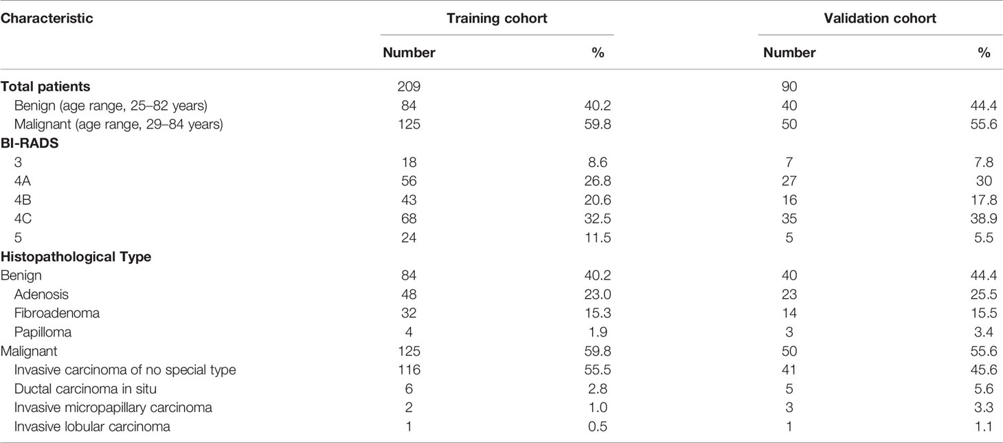
Table 1 Clinical characteristics of the patients selected for this study.
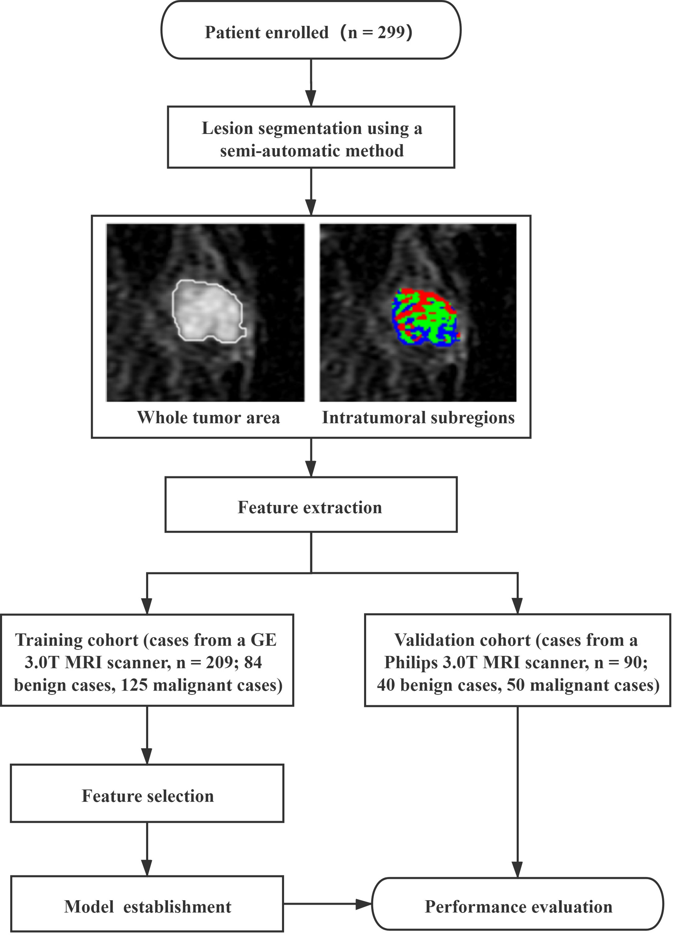
Figure 1 The flowchart adopted in this study.
Image Acquisition
In the training cohort, DCE-MRI examinations were performed with a GE 3.0T MRI scanner (Signa HDxt, GE Healthcare) equipped with a dedicated eight-channel bilateral breast coil on patients in a prone position. A transverse fat-suppression T1-weighted pre-contrast scan was first obtained with the VIBRANT-VX technique. Eight phases of fat-suppression T1-weighted post-contrast scans were acquired after intravenous injection of the contrast agent (Magnevist, Bayer-Schering Pharmaceuticals, Germany) at a dose of 0.15 mmol per kg body weight at 4 mlL/s and subsequent flushing with an equal volume of saline at the same injection speed. The following imaging parameters were used: repetition time (TR), 7.42 ms; echo time (TE), 4.25 ms; flip angle, 15°; slice thickness, 2.20 mm; spacing between slices, 2.20 mm; field of view, 340 × 340 mm2; image matrix, 1,024 × 1,024; slice number, 78. For each patient, eight phases of subtraction images were obtained by subtracting pre-contrast images from eight post-contrast images.
In the validation cohort, DCE-MRI examinations were performed with a Philips 3.0T MRI scanner (Ingenia, Philips Medical System, Best, Netherlands) equipped with a dedicated seven-channel bilateral breast coil with patient in a prone position. First, an axial fat-saturated T1-weighted pre-contrast scan was acquired. Then, eight axial contrast-enhanced fat-saturated T1-weighted scans were acquired after the intravenous bolus injection of the same contrast with the same dose. The imaging parameters were as follow: repetition time (TR), 4.14 ms; echo time (TE), 2.10 ms; flip angle, 12°; slice thickness, 2.00 mm; spacing between slices, 1.00 mm; field of view, 340 × 340 mm2; matrix, 380 × 380; slice number, 78. Eight subtraction sequences were obtained by subtracting the pre-contrast scan from each of the eight post-contrast scans.
Image Processing and Lesion Segmentation
Two senior radiologists, with 10 and 15 years of experience in interpreting breast MRI were invited to review the subtraction images in the fourth phase and reached a consensus in selecting the slice image with the maximum tumor diameter for each patient for subsequent analysis (27). During the image review, the radiologists were blind to the patients’ pathological results. The whole tumor area was segmented with a semi-automatic method in Matlab 2018b (Mathworks, Natick, MA, USA), as described below (28, 29). One of the two radiologists manually delineated a region of interest (ROI) with an arbitrary shape around the lesion area on the subtraction image. The pixel gray levels within the ROI were first normalized to μ ± 3σ (μ: mean gray level of pixels within the ROI; σ: standard deviation), and the range was quantized to 8 bits/pixel to change the signal to noise ratio of the texture results (30–32). A spatial fuzzy C-means (FCM) algorithm was then used to delineate the contour boundary of the lesion according to the ROI, and the whole lesion area was refined through morphological processing methods (33–35). Another radiologist verified and proofread the results of the semi-automatic breast tumor segmentation.
Intratumoral Subregion Partition
To better understand the intratumoral heterogeneity of breast tumors, as in a previous study (26), we divided the lesion area into three subregions according to the variations in pixel signal intensity in different phases. The specific partition details are as follows:
The relative enhancement of the post-contrast image compared with the pre-contrast image on a pixel-by-pixel basis was calculated with the following formula:
where I(m, n, t) and I(m, n t0) represent the signal intensity of the pixel (m, n) captured at times t and t0 (the pre-contrast moment) (36). The time-signal intensity curve, H(m, n, t), was defined to describe the variation in the relative enhancement over time (37–39). The time to peak (TTP), which represents the arrival time of the peak relative enhancement, was calculated with the following formula:
Then the pixels within the tumor region were divided into three subregions according to their TTP values. More specifically, pixel sets at the first four, fifth or sixth, and seventh or eighth phases to achieve peak enhancement values were defined as early, moderate, and late subregions, respectively; this method was similar to those described in previous studies (26, 36). Therefore, the tumor was divided into three regions representing different sets of TTP values.
Texture Feature Extraction
A total of 467 texture features were extracted from the whole tumor area and the three subregions with Matlab 2018b. The feature extraction methods could be classified into the following four categories: histogram, gray-level co-occurrence matrix (GLCM), gray-level run length matrix (GRLM), and discrete wavelet transform (DWT). Detailed information on the features is shown in Table 2. Each GLCM feature was calculated by using four angles (0, 45, 90, and 135°) and four distances (1, 2, 3, and 4 pixels). Each GRLM feature was calculated by using four angles (0, 45, 90, and 135°) and a distance of 1 pixel. In the following, (d, 0), (d, d), (0, d), and (-d, -d) were used to represent 0, 45, 90, and 135°, respectively, where d is the distance. Each DWT feature was calculated with four scales and three directions (horizontal, vertical, and diagonal) to generate low and high frequency components. In the following content, for example, Haar_2HH was used to represent the horizontal high frequency component of the second scale with the Haar wavelet.
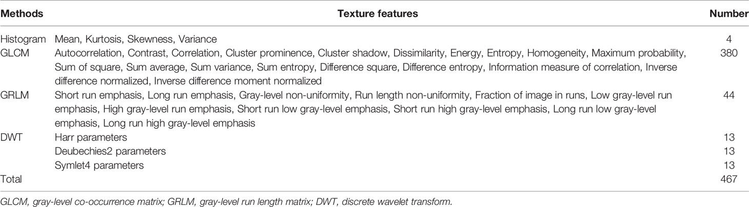
Table 2 Detailed information on the extracted features.
Feature Selection and Model Construction
To reduce the dimensionality of the features, the correlation between features was first tested with Pearson’s correlation analysis, and features with correlation coefficients of >0.95 relative to other features were removed. The remaining features were filtered by the least absolute shrinkage and selection operator (LASSO) method to select the optimal feature subset (40). Two machine learning models, decision tree (DT) and support vector machine (SVM), were used to construct classification models based on the optimal feature subset in the training cohort with a 10-fold cross-validation method for identifying benign and malignant breast tumors. And the classification models were tested by using a independent validation cohort. The 10-fold cross-validation refers to random division of the data set into 10 sets, nine of which were used for training and the last of which was used for testing. This process was repeated 10 times, and the test data differed each time.
Statistical Analysis
All statistical analyses were performed in SPSS 22.0 (IBM, Armonk, NY, USA). The Kolmogorov-Smirnov test was first performed on texture features selected by LASSO to assess whether the samples followed a normal distribution (41); if so, the variables in the tables are represented by means ± standard deviation (SD), and if not, the variables in the tables are represented by medians ± interquartile range. Univariate logistic regression analysis was used to evaluate the performance of an independent feature in distinguishing benign from malignant breast tumors. The receiver operating characteristic (ROC) curve constructed in the professional statistics software MedCalc (version 14.10.20, http://www.medcalc.org/) was used to assess the classification performance by calculating the area under the ROC curve (AUC). The corresponding accuracy, sensitivity, and specificity were also determined. The DeLong test was used to determine the statistical significance of differences between AUCs. A two-tailed P value of <0.05 was considered statistically significant.
The intraobserver variability of texture features extracted by the two radiologists was evaluated by using intraclass correlation coefficients [ICC, (0, 0.4), poor agreement; (0.4, 0.6), moderate agreement; (0.6, 0.8), good agreement; and (0.8, 1), excellent agreement] (42, 43).
Results
Study Cohort
A total of 299 patients were enrolled in this study. In the training cohort, the patients had 84 (40.2%) benign breast tumors classified into three histopathological types: adenosis (48), fibroadenoma (32), and papilloma (4). The 125 (59.8%) malignant breast tumors comprised 116 invasive carcinomas of no special type, 6 ductal carcinomas in situ, 2 invasive micropapillary carcinomas, and 1 invasive lobular carcinoma. In the validation cohort, the patients had 40 (44.4%) benign breast tumors classified into three histopathological types: adenosis (23), fibroadenoma (14), and papilloma (3). The 50 (55.6%) malignant breast tumors comprised 41 invasive carcinomas of no special type, 5 ductal carcinomas in situ, 3 invasive micropapillary carcinomas, and 1 invasive lobular carcinoma. The results of the whole tumor area segmentation and intratumoral subregion partition are displayed in Figure 2, which shows two randomly selected cases, one benign case and the other malignant case.
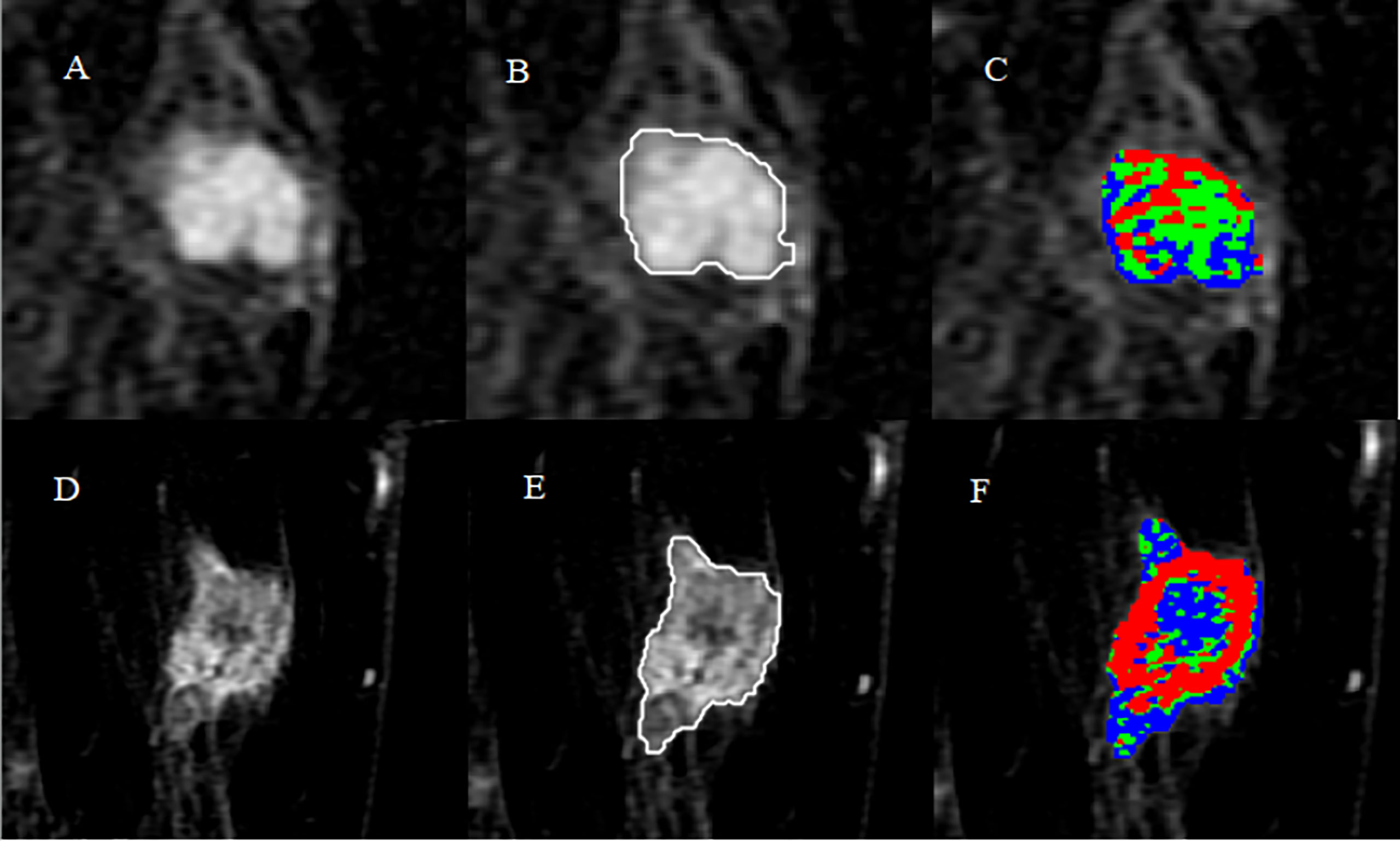
Figure 2 Results of whole tumor segmentation and intratumoral subregion partition. The first row shows the results of a benign case: (A) subtraction image with the maximum tumor diameter; (B) result of the whole tumor area segmented with a semi-automatic method; (C) result of intratumoral subregion partition, in which red, green, and blue represent the early, moderate, and late subregions, respectively. The second row shows the results of a malignant case: (D) subtraction image; (E) result of the whole tumor area; (F) result of intratumoral subregion partition.
Univariate Analysis
The results of univariate logistic regression analysis for identifying benign and malignant breast tumors are displayed in Table 3, which shows the top six features with the best performance extracted from the three subregions and the whole tumor area. The AUCs of features derived from the whole tumor area ranged from 0.732 to 0.786. Features from the early subregion performed best among the three subregions, with AUC values ranging from 0.787 to 0.886. The AUCs of the run length non-uniformity (1, 0) (P < 0.001), difference square (0, 1) (P = 0.004), and short run emphasis (1, 0) (P < 0.001) from the early subregion were significantly higher than those from the whole tumor area. The AUCs from the moderate subregion ranged from 0.715 to 0.777, and the AUCs from the late subregion ranged from 0.685 to 0.884. Among all individual features, the run length nonuniformity (1, 0) extracted from the early region achieved the highest AUC of 0.886 [95% confidence interval (CI), 0.836–0.926].
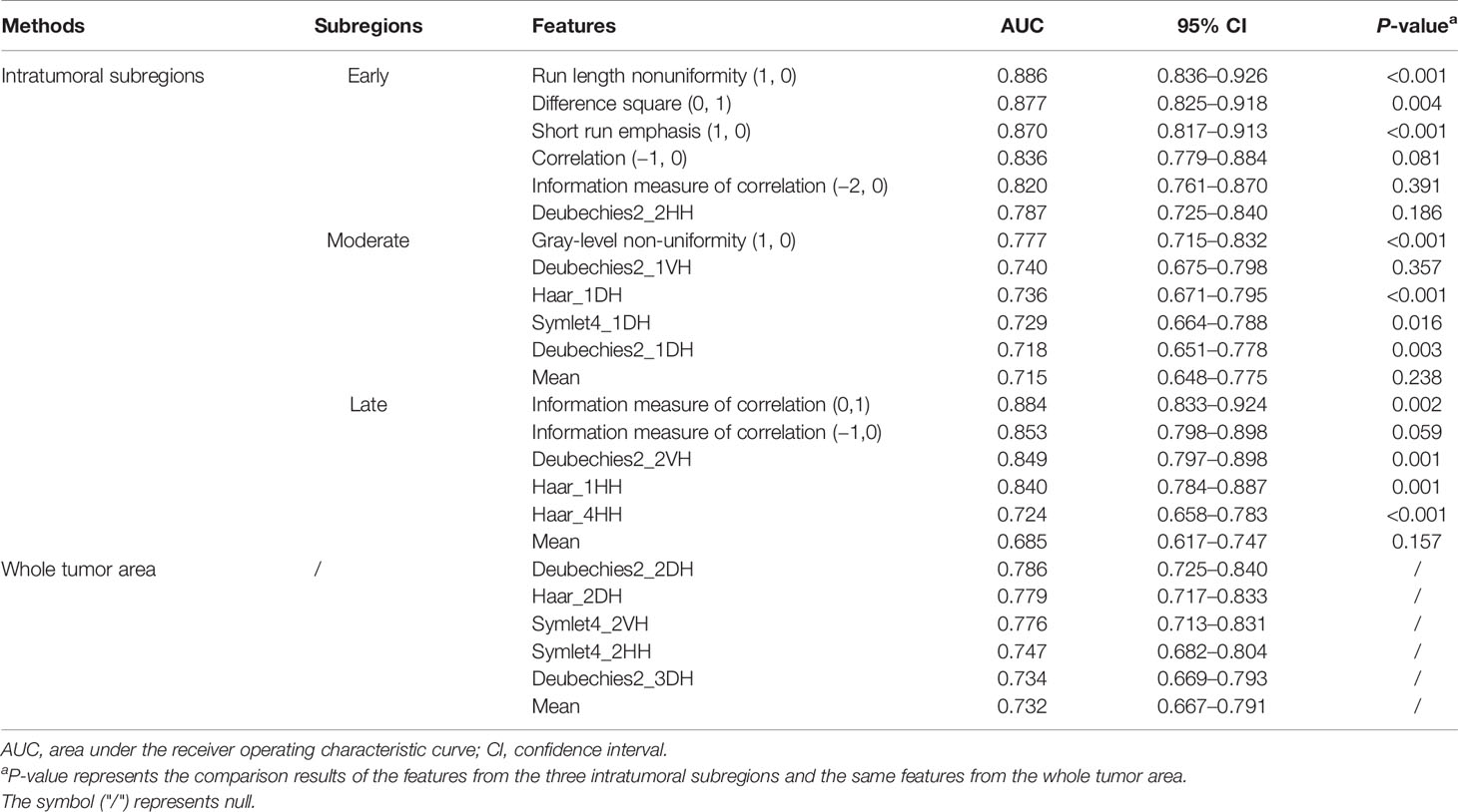
Table 3 Univariate analysis for predicting benign and malignant breast tumors.
Performance of Classification Models
Table 4 shows the performance of the classification models for distinguishing benign from malignant breast tumors in the training and validation cohorts, and the corresponding ROC curves are presented in Figures 3 and 4. In the training cohort, the AUCs of the DT_Whole model and SVM_Whole model were 0.744 and 0.806, respectively. In contrast, the AUCs of the DT_Early model (P = 0.004), DT_Late model (P = 0.015), SVM_Early model (P = 0.002), and SVM_Late model (P = 0.002) were significantly higher: 0.863 (95% CI, 0.808–0.906), 0.860 (95% CI, 0.806–0.904), 0.934 (95% CI, 0.891–0.963), and 0.921 (95% CI, 0.876–0.954), respectively. The SVM_Early model and SVM_Late model achieved better performance than the DT_Early model and DT_Late model (P = 0.003, 0.034, 0.008, and 0.026, respectively), as shown in Table 5. In the validation cohort, the AUCs of the DT_Whole model and SVM_Whole model were 0.670 and 0.708, respectively. In comparison, the AUCs of the DT_Early model (P = 0.006), DT_Late model (P = 0.043), SVM_Early model (P = 0.001), and SVM_Late model (P = 0.007) were significantly higher: 0.839 (95% CI, 0.747–0.908), 0.784 (95% CI, 0.601–0.798), 0.890 (95% CI, 0.806–0.946), and 0.865 (95% CI, 0.777–0.928), respectively. The SVM_Early model and SVM_Late model achieved better performance than the DT_Early model and DT_Late model (P = 0.018, 0.047, 0.035, and 0.029, respectively), as shown in Table 6. However, there was no significant difference between the SVM_Early model and the SVM_Late model in the training and validation cohorts (P = 0.524 and P = 0.523, respectively), and no significant difference between the DT_Early model and the DT_Late model (P = 0.945 and P = 0.332, respectively). Fifteen texture features extracted from the early subregion and 17 features extracted from the late subregion were selected by LASSO, as listed in Table 7.
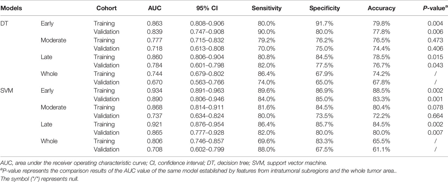
Table 4 Performance of classification models for identifying benign and malignant breast tumors.
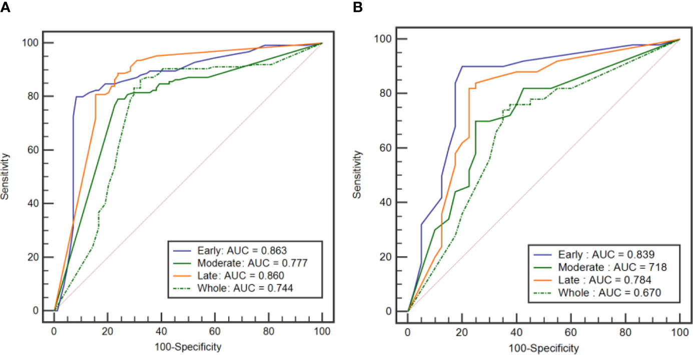
Figure 3 ROC curves of the DT classification models established by using the features extracted from the three intratumoral subregions and the whole tumor area. (A) ROC curves from the training cohort. (B) ROC curve from the external validation cohort.
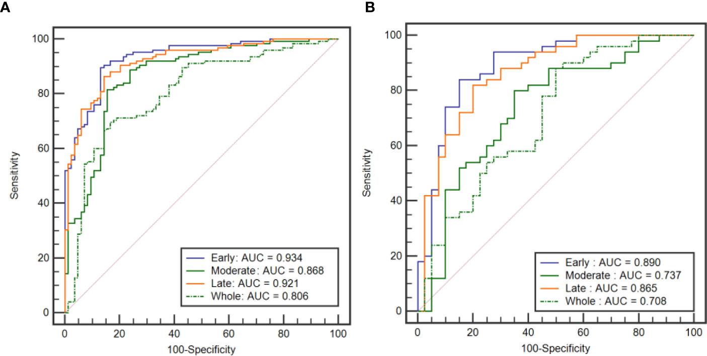
Figure 4 ROC curves of the SVM classification models established by using the features extracted from the three intratumoral subregions and the whole tumor area. (A) ROC curves from the training cohort. (B) ROC curves from the external validation cohort.
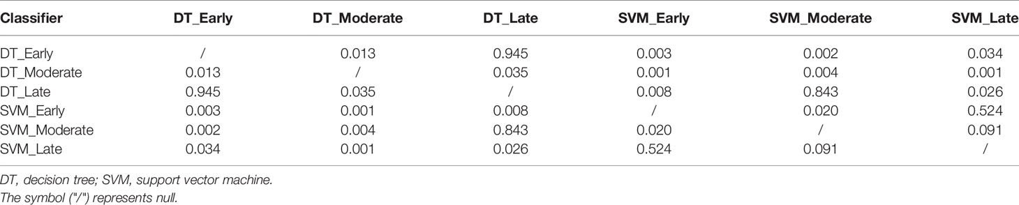
Table 5 P-values of DeLong tests between subregion models in the training cohort.

Table 6 P-values of DeLong tests between subregion models in the validation cohort.
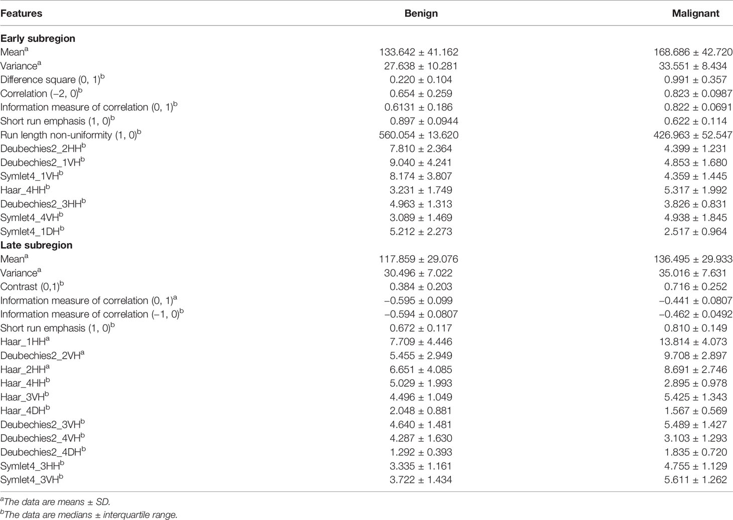
Table 7 Texture features extracted from early and late subregions selected with LASSO.
Interobserver Agreement Evaluation
The texture features derived from the two groups of ROIs delineated independently by two radiologists showed excellent agreement [ICCs for whole lesion region, (0.875, 0.943); ICCs for early region, (0.853, 0.936); ICCs for moderate region, (0.837, 0.928); and ICCs for late region, (0.842, 0.931)].
Discussion
This study investigated the relationship between texture features extracted from intratumoral subregions of breast DCE-MRI and the differential diagnosis of benign and malignant breast tumors. Features from subregions were able to distinguish benign from malignant breast tumors, and features from subregions representing the early and late TTP values achieved better performance than those from the whole tumor area in the training and validation cohorts. The SVM_Early model, SVM_Moderate model, and SVM_Late model demonstrated higher performance than the DT_Early model, DT_Moderate model, and DT_Late model, respectively.
Texture analysis can characterize intratumoral heterogeneity on the basis of quantitative image features extracted from conventional medical imaging to help diagnose, stage, and predict the prognosis and response to treatment in multiple oncology fields (44–46). Intratumoral heterogeneity reflects differences in biological characteristics, such as gene expression, metabolism, and angiogenesis (23, 47). Texture features derived from intratumoral subregions that reflect the heterogeneity of breast tumors, rather than the whole tumor area, may play a more important role in the prognostic analysis and identification of hormone receptor status in breast cancer (26, 36). A previous study has shown that texture features extracted from subregions with rapid delayed washout can be used to assess ER status and lymph node classification in breast cancer (48). Chang et al. (49) have quantified intratumoral heterogeneity on breast DCE-MRI by using a subregion-based feature extraction method for predicting ER status, human epidermal growth factor receptor 2 (HER2) status, and triple-negative breast cancer, achieving accuracy of 73.53, 82.35, and 77.45%, respectively. In this study, an intratumoral subregion partition method was used to distinguish benign from malignant breast tumors. Texture features were derived from three subregions and the whole tumor area, and the corresponding classification models were established. The models built with features from the early and late subregions achieved better performance than models built with features from the whole tumor area. A possible explanation for this finding is that the intratumoral subregions reflect angiogenesis, which may be indicative of the aggressiveness of malignant breast tumors (50).
A previous study has investigated the diagnostic performance of mammography texture analysis in differentiating benign from malignant breast tumors (51). In the present study, the subtraction images of DCE-MRI were used for texture analysis. Previous studies have discussed the roles of histograms, GLCM, and GRLM-based texture features in the differential diagnosis or treatment response assessment in breast cancer (14, 44). In addition to the features used in these studies, DWT-based features were extracted in this study. DWT is used to modify the image from the spatial domain to the frequency domain and has been extensively applied to feature extraction from electroencephalogram signals (52, 53). In the present univariate analysis, the DWT-based features derived from the late subregion, including Deubechies2_2VH (P = 0.001), Haar_1HH (P = 0.001), and Haar_4HH (P < 0.001), performed better in distinguishing benign from malignant breast tumors than those derived from the whole tumor area.
Two prevalent machine learning methods, DT and SVM, were applied to establish classification models in this study. To prevent overfitting, a 10-fold cross-validation method was used. The models established with features from the early and late subregions achieved better performance than models from the whole tumor area in the training and validation cohorts. However, no significant differences were found between the performance of models from the moderate subregion and that of models from the whole tumor area in the training and validation cohorts (P = 0.473 and P = 0.078, P = 0.406 and P = 0.664, respectively). Furthermore, the SVM_Early model, SVM_Moderate model, and SVM_Late model had higher AUCs than the DT_Early model, DT_Moderate model, and DT_Late model. SVM initially maps the input vector to a higher-dimensional feature space and identifies the hyperplane that divides the data points into two categories; the resulting classifier can reliably classify new samples and achieve considerable versatility (54).
A previous study by Li et al. (55) has applied four methods to classify benign and malignant breast tumors, and reported that the DT model achieved the best performance, with an AUC of 0.781, a sensitivity of 0.6, and a specificity of 0.894. Another study has used an SVM model for classifying benign and malignant breast tumors and obtained a sensitivity of 66.67% and a specificity of 93.55% (56). Wang et al. (20) have used logistic regression analysis to distinguish benign and malignant breast tumors, and achieved an accuracy of 79.5%, a sensitivity of 0.607, a specificity of 0.800, and an AUC of 0.802. In comparison, the best classification performance of our SVM_Early model achieved an AUC of 0.934, a sensitivity of 89.6%, a specificity of 86.9%, and an accuracy 88.5%. However, studies in which the classification model is based on deep learning methods have reported higher accuracy in distinguishing benign and malignant breast lesions (57, 58).
In addition, we separately evaluated the intraobserver variability of texture features extracted from the whole lesion region and from three different intratumoral subregions. The two radiologists showed high consistency in calculating texture features from the single-slice method, and all ICCs were greater than 0.8. The intraobserver variability was mainly related to slice selection and ROI delineation. Hence, standardized strategies for ROI determination are crucial.
This study has some limitations. First, the sample size was relatively small. Second, only a representative single-slice image was analyzed, and thus some useful information on the tumor might have been missed. Texture analysis based on three-dimensional breast tumor lesions may yield more useful information (59). Finally, the subtraction images of breast DCE-MRI were used to extract texture features. Features derived from post-contrast images or diffusion weighted imaging images may be helpful in distinguishing benign from malignant breast tumors (60).
Conclusion
The texture features extracted from intratumoral subregions of breast DCE-MRI can be used as imaging biomarkers for the differential diagnosis of benign from malignant breast tumors. Specifically, features derived from subregions representing the early and late TTP values achieved better performance than features from the whole tumor area. Further research with a larger sample size is needed to verify the results of this study.
Data Availability Statement
The original contributions presented in the study are included in the article/supplementary material. Further inquiries can be directed to the corresponding author.
Ethics Statement
The studies involving human participants were reviewed and approved by Shengjing Hospital of China Medical University. Written informed consent for participation was not required for this study in accordance with the national legislation and the institutional requirements. Written informed consent was not obtained from the individual(s) for the publication of any potentially identifiable images or data included in this article.
Author Contributions
Methodology, JY. Validation, LS. Investigation, BZ. Writing—original draft preparation, LS. Writing—review and editing, JY. Supervision, JY. Project administration, JY. Funding acquisition, JY. All authors contributed to the article and approved the submitted version.
Funding
This research was supported by grants from the Research and Development (R&D) Foundation for Major Science and Technology from Shenyang (No. 19-112-4-105), the Big Data Foundation for Health Care from China Medical University (No. HMB201902105), the Natural Fund Guidance Plan from Liaoning (No. 2019-ZD-0743), and the 345 Talent Project from Shengjing Hospital of China Medical University.
Conflict of Interest
The authors declare that the research was conducted in the absence of any commercial or financial relationships that could be construed as a potential conflict of interest.
References
1. Siegel RL, Miller KD, Jemal A. Cancer Statistics, 2020. CA Cancer J Clin (2020) 70(1):7–30. doi: 10.3322/caac.21590
2. Bayo J, Castaño MA, Rivera F, Navarro F. Analysis of Blood Markers for Early Breast Cancer Diagnosis. Clin Transl Oncol (2018) 20(4):467–75. doi: 10.1007/s12094-017-1731-1
3. Kunkler IH, Williams LJ, Jack WJ, Cameron DA, Dixon JM. Breast-Conserving Surgery With or Without Irradiation in Women Aged 65 Years or Older With Early Breast Cancer (PRIME II): A Randomised Controlled Trial. Lancet Oncol (2015) 16(3):266–73. doi: 10.1016/S1470-2045(14)71221-5
4. Lu Y, Chen Y, Zhu L, Cartwright P, Song E, Jacobs L, et al. Local Recurrence of Benign, Borderline, and Malignant Phyllodes Tumors of the Breast: A Systematic Review and Meta-Analysis. Ann Surg Oncol (2019) 26(5):1263–75. doi: 10.1245/s10434-018-07134-5
5. Grubstein A, Rapson Y, Stemmer SM, Allweis T, Wolff-Bar M, Borshtein S, et al. Timing to Imaging and Surgery After Neoadjuvant Therapy for Breast Cancer. Clin Imaging (2021) 71:24–8. doi: 10.1016/j.clinimag.2020.10.043
6. Heil J, Kuerer HM, Pfob A, Rauch G, Sinn HP, Golatta M, et al. Eliminating the Breast Cancer Surgery Paradigm After Neoadjuvant Systemic Therapy: Current Evidence and Future Challenges. Ann Oncol (2020) 31(1):61–71. doi: 10.1016/j.annonc.2019.10.012
7. Shien T, Iwata H. Adjuvant and Neoadjuvant Therapy for Breast Cancer. Jpn J Clin Oncol (2020) 50(3):225–9. doi: 10.1093/jjco/hyz213
8. Si L, Zhai R, Liu X, Yang K, Wang L, Jiang T. MRI in the Differential Diagnosis of Primary Architectural Distortion Detected by Mammography. Diagn Interv Radiol (2016) 22(2):141–50. doi: 10.5152/dir.2016.15017
9. Gubern-Mérida A, Vreemann S, Martí R, Melendez J, Lardenoije S, Mann RM, et al. Automated Detection of Breast Cancer in False-Negative Screening MRI Studies From Women at Increased Risk. Eur J Radiol (2016) 85(2):472–9. doi: 10.1016/j.ejrad.2015.11.031
10. Liu Z, Feng B, Li C, Chen Y, Chen Q, Li X, et al. Preoperative Prediction of Lymphovascular Invasion in Invasive Breast Cancer With Dynamic Contrast-Enhanced-MRI-Based Radiomics. J Magn Reson Imaging (2019) 50(3):847–57. doi: 10.1002/jmri.26688
11. Wang CH, Yin FF, Horton J, Chang Z. Review of Treatment Assessment Using DCE-MRI in Breast Cancer Radiation Therapy. World J Methodol (2014) 4(2):46–58. doi: 10.5662/wjm.v4.i2.46
12. Dalmış MU, Gubern-Mérida A, Vreemann S, Karssemeijer N, Mann R, Platel B. A Computer-Aided Diagnosis System for Breast DCE-MRI at High Spatiotemporal Resolution. Med Phys (2016) 43(1):84. doi: 10.1118/1.4937787
13. Pinker K, Helbich TH, Morris EA. The Potential of Multiparametric MRI of the Breast. Br J Radiol (2017) 90(1069):20160715. doi: 10.1259/bjr.20160715
14. Zhou J, Zhang Y, Chang KT, Lee KE, Wang O, Li J, et al. Diagnosis of Benign and Malignant Breast Lesions on DCE-MRI by Using Radiomics and Deep Learning With Consideration of Peritumor Tissue. J Magn Reson Imaging (2020) 51(3):798–809. doi: 10.1002/jmri.26981
15. Aker M, Ganeshan B, Afaq A, Wan S, Groves AM, Arulampalam T. Magnetic Resonance Texture Analysis in Identifying Complete Pathological Response to Neoadjuvant Treatment in Locally Advanced Rectal Cance. Dis Colon Rectum (2019) 62(2):163–70. doi: 10.1097/DCR.0000000000001224
16. Castellano G, Bonilha L, Li LM, Cendes F. Texture Analysis of Medical Images. Clin Radiol (2004) 59(12):1061–9. doi: 10.1016/j.crad.2004.07.008
17. Scalco E, Rizzo G. Texture Analysis of Medical Images for Radiotherapy Applications. Br J Radiol (2017) 90(1070):20160642. doi: 10.1259/bjr.20160642
18. Alobaidli S, McQuaid S, South C, Prakash V, Evans P, Nisbet A. The Role of Texture Analysis in Imaging as an Outcome Predictor and Potential Tool in Radiotherapy Treatment Planning. Br J Radiol (2014) 87(1042):20140369. doi: 10.1259/bjr.20140369
19. Mai H, Mao Y, Dong T, Tan Y, Huang X, Wu S, et al. The Utility of Texture Analysis Based on Breast Magnetic Resonance Imaging in Differentiating Phyllodes Tumors From Fibroadenomas. Front Oncol (2019) 9:1021. doi: 10.3389/fonc.2019.01021
20. Wang BT, Fan WP, Xu H, Li LH, Zhang XH, Wang K, et al. Value of Magnetic Resonance Imaging Texture Analysis in the Differential Diagnosis of Benign and Malignant Breast Tumors. Chin Med Sci J (2019) 34(1):33–7. doi: 10.24920/003516
21. Fan M, Zhang P, Wang Y, Peng W, Wang S, Gao X, et al. Radiomic Analysis of Imaging Heterogeneity in Tumours and the Surrounding Parenchyma Based on Unsupervised Decomposition of DCE-MRI for Predicting Molecular Subtypes of Breast Cancer. Eur Radiol (2019) 29(8):4456–67. doi: 10.1007/s00330-018-5891-3
22. Carvalho ED, Filho AOC, Silva RRV, Araújo FHD, Diniz JOB, Silva AC, et al. Breast Cancer Diagnosis From Histopathological Images Using Textural Features and CBI. Artif Intell Med (2020) 105:101845. doi: 10.1016/j.artmed.2020.101845
23. Marusyk A, Polyak K. Tumor Heterogeneity: Causes and Consequences. Biochim Biophys Acta (2010) 1805(1):105–17. doi: 10.1016/j.bbcan.2009.11.002
24. Kavya N, Sriraam N, Usha N, Bharathi H, Anusha S, Sharath D, et al. Breast Cancer Lesion Detection From Cranial-Caudal View of Mammogram Images Using Statistical and Texture Features Extractio. Int J Biomed Clin Eng (IJBCE) (2020) 9(1):16–32. doi: 10.4018/IJBCE.2020010102
25. Fujiwara T, Urata Y, Tanaka N. Telomerase-Specific Oncolytic Virotherapy for Human Cancer With the hTERT Promoter. Curr Cancer Drug Targets (2007) 7(2):191–201. doi: 10.2174/156800907780058835
26. Fan M, Cheng H, Zhang P, Gao X, Zhang J, Shao G, et al. DCE-MRI Texture Analysis With Tumor Subregion Partitioning for Predicting Ki-67 Status of Estrogen Receptor-Positive Breast Cancers. J Magn Reson Imaging (2018) 48(1):237–47. doi: 10.1002/jmri.25921
27. Wang TC, Huang YH, Huang CS, Chen JH, Huang GY, Chang RF. Computer-Aided Diagnosis of Breast DCE-MRI Using Pharmacokinetic Model and 3-D Morphology Analysis. Magn Reson Imaging (2014) 32(3):197–205. doi: 10.1016/j.mri.2013.12.002
28. Ren H, Zhou L, Liu G, Peng X, Shi W, Xu H, et al. An Unsupervised Semi-Automated Pulmonary Nodule Segmentation Method Based on Enhanced Region Growing. Quant Imaging Med Surg (2020) 10(1):233–42. doi: 10.21037/qims.2019.12.02
29. Liney GP, Gibbs P, Hayes C, Leach MO, Turnbull LW. Dynamic Contrast-Enhanced MRI in the Differentiation of Breast Tumors: User-Defined Versus Semi-Automated Region-of-Interest Analysis. J Magn Reson Imaging (1999) 10(6):945–9. doi: 10.1002/(sici)1522-2586(199912)10:6<945::aid-jmri6>3.0.co;2-i
30. Collewet G, Strzelecki M, Mariette F. Influence of MRI Acquisition Protocols and Image Intensity Normalization Methods on Texture Classification. Magn Reson Imaging (2004) 22:81–91. doi: 10.1016/j.mri.2003.09.001
31. Wang H, Nie P, Wang Y, Xu W, Duan S, Chen H, et al. Radiomics Nomogram for Differentiating Between Benign and Malignant Soft-Tissue Masses of the Extremities. J Magn Reson Imaging (2020) 51:155–63. doi: 10.1002/jmri.26818
32. Gibbs P, Turnbull LW. Textural Analysis of Contrast-Enhanced MR Images of the Breast. Magn Reson Med (2003) 50:92–8. doi: 10.1002/mrm.10496
33. Wang C, Pedrycz W, Yang J, Zhou M, Li Z. Wavelet Frame-Based Fuzzy C-Means Clustering for Segmenting Images on Graph. IEEE Trans Cybern (2020) 50(9):3938–49. doi: 10.1109/TCYB.2019.2921779
34. Boudraa AE, Champier J, Cinotti L, Bordet JC, Lavenne F, Mallet JJ. Delineation and Quantitation of Brain Lesions by Fuzzy Clustering in Positron Emission Tomography. Comput Med Imaging Graph (1996) 20(1):31–41. doi: 10.1016/0895-6111(96)00025-0
35. Khan SU, Ullah I, Ahmed I, Imran A, Ullah N. A Spatial Fuzzy C-Means Algorithm for Segmentation of Brain MRI Images. J X-ray Sci Technol (2019) 27(6):1087–99. doi: 10.3233/XST-190547
36. Ashraf A, Gaonkar B, Mies C, DeMichele A, Rosen M, Davatzikos C, et al. Breast DCE-MRI Kinetic Heterogeneity Tumor Markers: Preliminary Associations With Neoadjuvant Chemotherapy Response. Transl Oncol (2015) 8(3):154–62. doi: 10.1016/j.tranon.2015.03.005
37. Gu J, Polley EC, Denis M, Carter JM, Pruthi S, Gregory AV, et al. Early Assessment of Shear Wave Elastography Parameters Foresees the Response to Neoadjuvant Chemotherapy in Patients With Invasive Breast Cancer. Breast Cancer Res (2021) 23(1):52. doi: 10.1186/s13058-021-01429-4
38. Hylton N. MR Imaging for Assessment of Breast Cancer Response to Neoadjuvant Chemotherapy. Magn Reson Imaging Clin N Am (2006) 14(3):383–9, vii. doi: 10.1016/j.mric.2006.09.001
39. Lee SH, Kim JH, Cho N, Park JS, Yang Z, Jung YS, et al. Multilevel Analysis of Spatiotemporal Association Features for Differentiation of Tumor Enhancement Patterns in Breast DCE-MR. Med Phys (2010) 37(8):3940–56. doi: 10.1118/1.3446799
40. Yamada M, Jitkrittum W, Sigal L, Xing EP, Sugiyama M. High-Dimensional Feature Selection by Feature-Wise Kernelized Lass. Neural Comput (2014) 26(1):185–207. doi: 10.1162/NECO_a_00537
41. Field A. Discovering Statistics Using IBM SPSS Statistics.4th ed. New Delhi: Sage Publications Ltd (2013).
42. Liu L, Liu Y, Xu L, Li Z, Lv H, Dong N, et al. Application of Texture Analysis Based on Apparent Diffusion Coefficient Maps in Discriminating Different Stages of Rectal Cancer. J Magn Reson Imaging (2017) 45:1798–808. doi: 10.1002/jmri.25460
43. Yang L, Liu D, Fang X, Wang Z, Xing Y, Ma L, et al. Rectal Cancer: Can T2WI Histogram of the Primary Tumor Help Predict the Existence of Lymph Node Metastasis? Eur Radiol (2019) 29:6469–76. doi: 10.1007/s00330-019-06328-z
44. Ahmed A, Gibbs P, Pickles M, Turnbull L. Texture Analysis in Assessment and Prediction of Chemotherapy Response in Breast Cancer. J Magn Reson Imaging (2013) 38(1):89–101. doi: 10.1002/jmri.23971
45. Guan Y, Li W, Jiang Z, Chen Y, Liu S, He J, et al. Whole-Lesion Apparent Diffusion Coefficient-Based Entropy-Related Parameters for Characterizing Cervical Cancers: Initial Findings. Acad Radiol (2016) 23(12):1559–67. doi: 10.1016/j.acra.2016.08.010
46. Ryu YJ, Choi SH, Park SJ, Yun TJ, Kim JH, Sohn CH. Glioma: Application of Whole-Tumor Texture Analysis of Diffusion-Weighted Imaging for the Evaluation of Tumor Heterogeneity. PloS One (2014) 9(9):e108335. doi: 10.1371/journal.pone.0108335
47. Bedard PL, Hansen AR, Ratain MJ, Siu LL. Tumour Heterogeneity in the Clinic. Nature (2013) 501(7467):355–64. doi: 10.1038/nature12627
48. Chaudhury B, Zhou M, Goldgof DB, Hall LO, Gatenby RA, Gillies RJ, et al. Heterogeneity in Intratumoral Regions With Rapid Gadolinium Washout Correlates With Estrogen Receptor Status and Nodal Metastasis. J Magn Reson Imaging (2015) 42(5):1421–30. doi: 10.1002/jmri.24921
49. Chang RF, Chen HH, Chang YC, Huang CS, Chen JH, Lo CM. Quantification of Breast Tumor Heterogeneity for ER Status, HER2 Status, and TN Molecular Subtype Evaluation on DCE-MR. Magn Reson Imaging (2016) 34(6):809–19. doi: 10.1016/j.mri.2016.03.001
50. Li L, Wang K, Sun X, Wang K, Sun Y, Zhang G, et al. Parameters of Dynamic Contrast-Enhanced MRI as Imaging Markers for Angiogenesis and Proliferation in Human Breast Cancer. Med Sci Monit (2015) 21:376–82. doi: 10.12659/MSM.892534
51. Li Z, Yu L, Wang X, Yu H, Gao Y, Ren Y, et al. Diagnostic Performance of Mammographic Texture Analysis in the Differential Diagnosis of Benign and Malignant Breast Tumors. Clin Breast Cancer (2018) 18(4):e621–7. doi: 10.1016/j.clbc.2017.11.004
52. Ashraf R, Ahmed M, Jabbar S, Khalid S, Ahmad A, Din S, et al. Content Based Image Retrieval by Using Color Descriptor and Discrete Wavelet Transform. J Med Syst (2018) 42(3):44. doi: 10.1007/s10916-017-0880-7
53. Al-Fahoum AS, Al-Fraihat AA. Methods of EEG Signal Features Extraction Using Linear Analysis in Frequency and Time-Frequency Domains. ISRN Neurosci (2014) 2014:730218. doi: 10.1155/2014/730218
54. Kourou K, Exarchos TP, Exarchos KP, Karamouzis MV, Fotiadis DI. Machine Learning Applications in Cancer Prognosis and Prediction. Comput Struct Biotechnol J (2014) 13:8–17. doi: 10.1016/j.csbj.2014.11.005
55. Li K, Wang Q, Lu Y, Pan X, Liu L, Cheng S, et al. Machine Learning Based Tissue Analysis Reveals Brachyury has a Diagnosis Value in Breast Cancer. Biosci Rep (2021) 41(4):BSR20203391. doi: 10.1042/BSR20203391
56. Liu Y, Ren Li, Cao X, Tong Y. Breast Tumors Recognition Based on Edge Feature Extraction Using Support Vector Machine. Biomed Biomed Signal Process Control [Preprint] (2020) 58. doi: 10.1016/j.bspc.2019.101825
57. Krithiga R, Geetha P. Deep Learning Based Breast Cancer Detection and Classification Using Fuzzy Merging Techniques. Mach Vision Appl (2020) 31(7):1–18. doi: 10.1007/s00138-020-01122-0
58. Aslam MA, Aslam, Daxiang C. Breast Cancer Classification Using Deep Convolutional Neural Networ. J Phys: Conf Ser (2020) 1584(1):012005–. doi: 10.1088/1742-6596/1584/1/012005
59. Zhou J, Luo LY, Dou Q, Chen H, Chen C, Li GJ, et al. Weakly Supervised 3D Deep Learning for Breast Cancer Classification and Localization of the Lesions in MR Images. J Magn Reson Imaging (2019) 50(4):1144–51. doi: 10.1002/jmri.26721
Keywords: breast tumors, magnetic resonance imaging, machine learning, texture analysis, DCE-MRI
Citation: Zhang B, Song L and Yin J (2021) Texture Analysis of DCE-MRI Intratumoral Subregions to Identify Benign and Malignant Breast Tumors. Front. Oncol. 11:688182. doi: 10.3389/fonc.2021.688182
Received: 30 March 2021; Accepted: 15 June 2021;
Published: 08 July 2021.
Edited by:
Chuanming Li, Chongqing Medical University, ChinaCopyright © 2021 Zhang, Song and Yin. This is an open-access article distributed under the terms of the Creative Commons Attribution License (CC BY). The use, distribution or reproduction in other forums is permitted, provided the original author(s) and the copyright owner(s) are credited and that the original publication in this journal is cited, in accordance with accepted academic practice. No use, distribution or reproduction is permitted which does not comply with these terms.
*Correspondence: Jiandong Yin, amlhbmRvbmd5aW5Ac2luYS5jb20=