 Dhruv Gopalakrishnan1,2,3*
 Luca Dellantonio1,4,5*
 Antonio Di Pilato6*Wahid Redjeb6,7*
 Felice Pantaleo6*Michele Mosca1,3,4,8*
- 1Institute for Quantum Computing, University of Waterloo, Waterloo, ON, Canada
- 2Department of Electrical and Computer Engineering, University of Waterloo, Waterloo, ON, Canada
- 3Perimeter Institute of Theoretical Physics, Waterloo, ON, Canada
- 4Department of Physics and Astronomy, University of Waterloo, Waterloo, ON, Canada
- 5Department of Physics and Astronomy, University of Exeter, Exeter, United Kingdom
- 6CERN, Geneva, Switzerland
- 7RWTH Aachen University Physikalisches Institut III A, Aachen, Germany
- 8Department of Combinatorics and Optimization, University of Waterloo, Waterloo, ON, Canada
Clustering algorithms are at the basis of several technological applications, and are fueling the development of rapidly evolving fields such as machine learning. In the recent past, however, it has become apparent that they face challenges stemming from datasets that span more spatial dimensions. In fact, the best-performing clustering algorithms scale linearly in the number of points, but quadratically with respect to the local density of points. In this work, we introduce qCLUE, a quantum clustering algorithm that scales linearly in both the number of points and their density. qCLUE is inspired by CLUE, an algorithm developed to address the challenging time and memory budgets of Event Reconstruction (ER) in future High-Energy Physics experiments. As such, qCLUE marries decades of development with the quadratic speedup provided by quantum computers. We numerically test qCLUE in several scenarios, demonstrating its effectiveness and proving it to be a promising route to handle complex data analysis tasks – especially in high-dimensional datasets with high densities of points.
1 Introduction
Clustering is a data analysis technique that is crucial in several fields, owing to its ability to uncover hidden patterns and structures within large datasets (Gopalakrishnan et al., 2024). It is essential for simplifying complex data, improving data organization, and enhancing decision-making processes (Oyelade et al., 2019; Gu and Hübschmann, 2022; Caruso et al., 2018; Wu et al., 2021). For instance, clustering has been applied in marketing (Huang et al., 2007; Punj and Stewart, 1983), where it helps segment customers for targeted advertising (Wu et al., 2009), and in biology, for classifying genes and identifying protein interactions (Dutta et al., 2020; Au et al., 2005; Wang et al., 2010; Asur et al., 2007). In the realm of computer science and artificial intelligence, it is invaluable for speech recognition (Kishore Kumar et al., 2018; Chang et al., 2017), image segmentation (Coleman and Andrews, 1979), as well as for recommendation systems (Shepitsen et al., 2008; Schickel-Zuber and Faltings, 2007) used for personalizing user content. Finally, clustering techniques are pivotal for Event Reconstruction (ER), where data points that originated from the same “event” are to be grouped together. In High-Energy Physics, for instance, clustering algorithms are used to reconstruct the trajectories of subatomic particles in collider experiments. High volumes of data are expected at the endcap High Granularity CALorimeter (HGCAL) (Didier and Austin, 2017) which is currently being built for the CMS detector at the High Luminosity Large Hadron Collider (HL-LHC). This must be tackled by new generations of clustering algorithms such as CLUE (Rovere et al., 2020). The discovery of the Higgs boson (Aad et al., 2012), awarded the Nobel prize in 2012, was made possible by such algorithms.
ER enables the interpretation of data obtained from particle collision events, including those occurring at the Large Hadron Collider (LHC) at CERN. Several clustering algorithms like DBScan, K-Means, and Hierarchical Clustering among others (Amaro et al., 2023; Dalitz et al., 2019; Rodenko et al., 2019) can be employed for ER. Our work is based on CERN’s CLUstering of Energy (CLUE) algorithm (Rovere et al., 2020; CMS Collaboration, 2022), which is adopted by the CMS collaboration (Hayrapetyan et al., 2023; Hayrapetyan et al., 2024; Tumasyan et al., 2023). It is designed for the future HGCAL detector due to the limitations of the currently employed algorithms. Despite these limitations, such algorithms are already at the basis of several discoveries, such as the doubly charged tetraquark (Aaij et al., 2023), the study of rare B meson decays to two muons (Tumasyan et al., 2023) and the observation of four-top quark production in proton-proton collisions (Hayrapetyan et al., 2023).
The efficiency of clustering algorithms, as illustrated by the CLUE algorithm (Rovere et al., 2020), is crucial for handling large datasets. Initially designed for two-dimensional datasets, CLUE reduces the search complexity from
In the context of CLUE, where the datasets in question are limited to two dimensions,
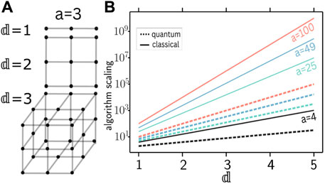
Figure 1. Scaling of point density and complexities of classical and quantum algorithms for the unstructured search problem with dimension
A first step towards extending CLUE to more dimensions is 3D-CLUE (Rovere et al., 2020; Brondolin, 2022). In this work, data points from different detector layers are first projected onto a single
Quantum computers provide a route to mitigate the complexity blow-up arising from higher-dimensional datasets. Wei et al. (2020) addresses the task of jet clustering in High-Energy Physics, while Kerenidis and Landman (2021) targets spectral clustering, which itself uses the efficient quantum analogue of
In this work we develop qCLUE, a CLUE-inspired quantum algorithm. Similarly to other quantum algorithms (Nicotra et al., 2023; Tüysüz et al., 2020), qCLUE leverages the advantage provided by Grover Search (Lov, 1996). A comparison of classical and quantum (Grover) runtimes is presented in Figure 1B, where the solid [dashed] lines refer to the classical
Overall, we find that qCLUE performs well in a wide range of scenarios. With ER-inspired datasets as a specific example, we demonstrate that clusters are correctly reconstructed in typical experimental settings. Similar to other quantum approaches to clustering that rely on Grover Search (Aïmeur et al., 2007; Pires et al., 2021; Magano et al., 2022), qCLUE showcases a quadratic speedup compared to classical algorithms. Magano et al. (2022) is especially interesting as it provides a detailed computational complexity analysis to a related problem within ER. Specifically, this approach tackles a subsequent task compared to qCLUE, namely the creation of so-called tracksters from hits (CMS Collaboration, 2022). It also demonstrates that the quantum algorithm has a quadratic advantage if compared to the classical one in physically relevant scenarios. We mention here the significance of variational solutions (Zlokapa et al., 2021; Tüysüz et al., 2021) to the ER reconstruction problem but note that these do not have predictable runtimes or error bound guarantees.
The specific advantages of qCLUE are its CLUE-inspired approach to cluster reconstruction (which demonstrated to be extremely successful (CMS Collaboration, 2022; Hayrapetyan et al., 2023; Tumasyan et al., 2023; CMS Collaboration, 2024)), and its consequent seamless integration with the classical framework currently employed by the CMS collaboration (Rovere et al., 2020; Brondolin, 2022; CMS Collaboration, 2023).
This paper is structured as follows. In Section 2, we describe our algorithm qCLUE. Specifically, we provide a general overview of its subroutines – namely the Compute Local Density, Find Nearest Higher, and the Find Seeds, Outliers and Assign Clusters steps. We describe the results of our simulated version of qCLUE on a classical computer in Section 3. In more detail, we explain the scoring metrics we use to quantify our results, and describe qCLUE performance when the dataset is subject to noise and different clusters overlap. Conclusions and outlook are finally presented in Section 4.
2 qCLUE
qCLUE is a quantum adaptation of CERN’s CLUE and 3D-CLUE algorithms (Rovere et al., 2020; Brondolin, 2022), that is specifically developed for ER, yet it is suitable to work with any (high dimensional) dataset. The main advantage of qCLUE stems from employing Grover’s algorithm, which provides a quadratic speedup for the Unstructured Search Problem (Lov, 1996). While qCLUE is designed to work in arbitrary dimensions, for clarity we restrict ourselves to
In Section 2.1, we offer an overview of the algorithm and its different subroutines. Section 2.2 is dedicated to the first subroutine of qCLUE, namely, calculating the Local Density. We then explain how to determine the Nearest Highers
2.1 Overview and setting
As for CLUE and 3D-CLUE (Rovere et al., 2020; Brondolin, 2022), we consider a dataset with spatial coordinates and an weight for every point. Similar datasets can also be found in medical image analysis and segmentation (Qaqish et al., 2017; Ng et al., 2006), in the analysis of asteroid reflectance spectra and hyperspectral astronomical imagery in astrophysics (Galluccio et al., 2008; Gaffey, 2010; Gao et al., 2021) and in gene analysis in bioinformatics (Karim et al., 2020; Oyelade et al., 2016).
In
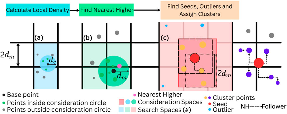
Figure 2. Pictorial representation of the main subroutines of qCLUE. In (A), the Local Density computation subroutine is represented. The consideration circle of radius
In this work, we employ a qRAM to store and access data, which is an essential building block for quantum computers. Following Giovannetti et al. (2008), we therefore assume that we can efficiently prepare the state.
where
The qCLUE algorithm consists of the following steps:
2.1.1 Local density
The first step is to calculate the local density
and it is indicative of the weight in a neighborhood of point
2.1.2 Find nearest higher
After calculating the local densities, we determine the nearest highers. The Nearest Higher
2.1.3 Find seeds, outliers and assign clusters
As schematically represented in Figure 2C, seeds (red points) are the points whose distance
Here,
Once seeds and outliers are determined, the clusters are constructed. From the seeds, we iteratively combine “followers.” If point
2.2 Local density computation
In this section, we describe the subroutine (schematically represented in Figure 3) that computes the Local Density
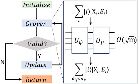
Figure 3. Algorithm flow for Local Density computation and for Assigning Clusters. The quantum state is initialized in the green “Initialize” box. For Local Density Computation (Cluster Assignment), it comprises all points in the DSS
We shall refer to
where the index
At this stage, we must find the points
Here, the first register of the Grover output contains all points characterized by indices
When the algorithm is run, measurement either yields a point that satisfies this distance condition, or (if there are no valid indices left) an index that does not satisfy this condition. This is verified by the grey “Valid?” diamond in Figure 3. The branched logic following this block ensures that the algorithm loops until all the required points are returned by the algorithm in the “Return” block.
Once we have obtained all indices
The scaling of the subroutine that determines the local density of a single point is given by the number of points in the blue consideration circle in Figure 2A such that
As a final remark, we highlight that it is in principle possible to design a unitary that computes the Local Density directly and stores the output in a quantum register. This unitary would remove the requirement of finding individually the indices
2.3 Find nearest higher
Here, we describe qCLUE’s subroutine for finding the Nearest Highers
Similar to the initialization carried out for the Local Density Computation step, we use qRAM to initialize the quantum state
Here, the indices
To find the Nearest Higher, we use a Grover-Enhanced Binary Search (GEBS) where each search step is enhanced by Grover’s algorithm (Equation 5). The output of every Grover run,
is a superposition over all points
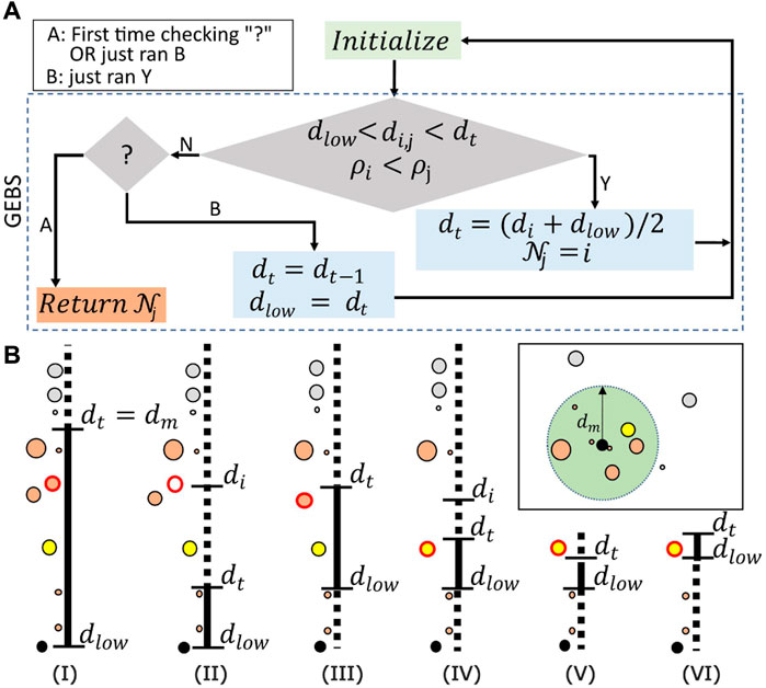
Figure 4. (A) Diagrammatic representation of the algorithm. GEBS determines successive candidates for the “Nearest Higher” until the proper one is found. The quantum state in Equation 6 is prepared in the “Initialize” step (green box). Grover Search (larger diamond) is then performed to find the points satisfying
To better understand the algorithm, we provide a step-by-step walkthrough of the example in Figure 4B. The search space
GEBS starts with the higher threshold set as
Now, assume that the new point with a red border is found [step (III)]. Updates in the
The runtime complexity of the GEBS procedure, with
2.4 Find seeds, outliers, and assign clusters
Once the Nearest Highers
Similar to the previous subroutines, the quantum registers for these procedures are initialized via qRAM. Seeds and outliers are then determined based on the corresponding conditions via Grover Search. Two quantum registers, the first marking whether a point is an outlier and the second to store the seed number – which is also the cluster number – are added to the quantum database.
The final subroutine of qCLUE is the assignment of points to clusters. At this stage, outliers have been removed from the input dataset, as they have been already identified. The algorithm flow is the same as that of the Local Density step in Figure 3. For a chosen seed
In the “Grover” block, we search over a superposition of points in the dataset which we call the Dynamic Search Space (DSS) created by qRAM as shown in Equations 8a, 8b. The DSS differs from the search space
With a similar procedure as for the Local Density subroutine, the “Grover” block now systematically identifies all followers of all points within set
The complexity of the Cluster Assignment step is similar to the one of the Local Density Computation subroutine. The quantum advantage stems from the quadratic speedup provided by the Grover algorithm, which allows determining the follower faster if compared to CLUE. If there are
3 Results
In this section, we test qCLUE in multiple scenarios, each designed to investigate its performance for different settings. In Section 3.1, we introduce the scoring metrics used for our analysis. In Section 3.2, we describe the performance of the algorithm applied on a single cluster in a uniform noisy environment. In Section 3.3, we study the performance on overlapping clusters. Finally, in Section 3.4, we study the performance of qCLUE on non-centroidal clusters with and without a weight profile.
3.1 Scoring metrics: homogeneity and completeness scores
It is more important to correctly classify high-weight points such as seeds as compared to low-weight points such as outliers. Since we would like our metric to be cognizant to this, we use modified, weight-aware versions (Jekaterina, 2023) of the Homogeneity
As discussed in (Jekaterina, 2023),
qCLUE applied to an input dataset yields homogeneity
3.2 Noise
Here, we study the performance of qCLUE for a single cluster in a noisy environment. We vary the number
where
Examples of the generated clusters (in orange) and noise (in blue) are given in Figures 5A, B for
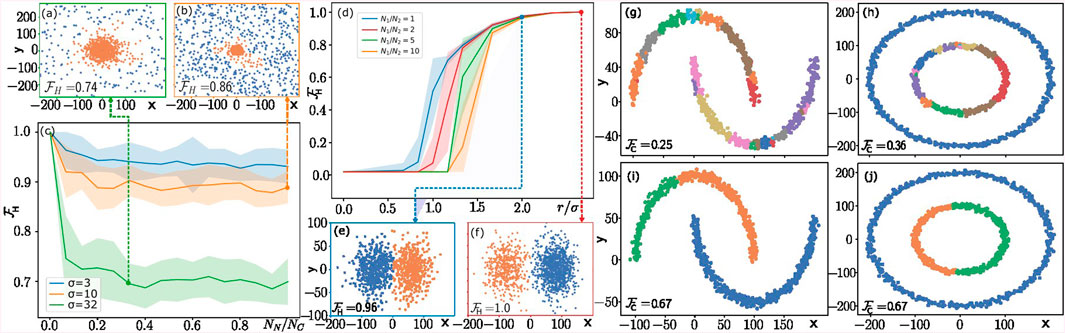
Figure 5. Numerical results from qCLUE simulated on a classical machine. (A–C) qCLUE’s performance in noisy environments. The dataset generated for these experiments and visualized in panels (A, B) consists of a cluster (noise) with
In Figure 5C, we show the variation of homogeneity score
3.3 Overlap
Here, we consider the case of two circular clusters with
In Figure 5D, we study the variation of homogeneity score
For all
The performance of qCLUE is also affected by the ratio
3.4 Non-centroidal clusters
Finally, we study the performance of qCLUE on non-centroidal clusters. For this purpose, we use the Moons and Circles datasets in Figures 5G–J, generated using
In the latter case, we assign the highest value of the weight for each cluster to a single point and lower the weights of all other points proportionally to their
Since these datasets are noiseless and well separated,
4 Conclusion and outlook
We introduced qCLUE, a novel quantum clustering algorithm designed to address the computational challenges associated with high-dimensional datasets. qCLUE’s significance lies in its potential to efficiently cluster data by effectively leveraging quantum computing, mitigating the escalating computational complexity encountered by classical algorithms upon increasing dimensionality of datasets. The algorithm’s ability to navigate high-dimensional spaces is particularly promising on datasets with high point density, where local searches become too demanding for classical computers. Therefore, qCLUE will be beneficial in multiple scenarios, ranging from quantum-enhanced machine learning (Haug et al., 2023; Zeguendry et al., 2023) to complex data analysis tasks (Sinayskiy et al., 2015).
According to our numerical results, qCLUE works well and its performance is significantly enhanced when a weight profile is assigned. Specifically, we study qCLUE in noisy environments, on overlapping clusters, and on non-centroidal datasets that are commonly used to benchmark clustering algorithms (Fujita, 2021; Tiwari et al., 2020). In scenarios that are typically encountered in ER tasks, qCLUE correctly reconstructs the true clusters to a high level of accuracy as it matches the performance of CERN’s CLUE on a given dataset. On the other hand, a weight profile can significantly boost qCLUE performance as we have seen in the case of non-centroidal clusters. Our numerical results, backed up by the well-studied CLUE and by the quadratic speedup stemming from Grover search, make qCLUE a promising candidate for addressing high-dimensional clustering problems (Wei et al., 2020; Kerenidis and Landman, 2021; Duarte et al., 2023).
As a first outlook, we identify the implementation of qCLUE on NISQ hardware (Celi et al., 2020; Labuhn et al., 2016; Bernien et al., 2017; Lanyon et al., 2011; Arute et al., 2019; Córcoles et al., 2015; Debnath et al., 2016). This requires a comprehensive consideration of real device constraints. Aspects such as circuit optimization (Nash et al., 2020), and the impact of noise will be critical and must be carefully addressed. Second, it is possible to improve the scaling of qCLUE by devising a unitary that mitigates the need for repeating Grover’s algorithm for each point satisfying the search condition and thereby eliminating the factors of
Data availability statement
The datasets presented in this study can be found in online repositories. The names of the repository/repositories and accession number(s) can be found below: https://zenodo.org/records/12655189.
Author contributions
DG: Writing–original draft, Writing–review and editing. LD: Writing–original draft, Writing–review and editing. AD: Writing–original draft, Writing–review and editing. WR: Writing–original draft, Writing–review and editing. FP: Writing–original draft, Writing–review and editing. MM: Writing–original draft, Writing–review and editing.
Funding
The author(s) declare that financial support was received for the research, authorship, and/or publication of this article. CERN Quantum Initiative. Wolfgang Gentner Programme of the German Federal Ministry of Education and Research (grant no. 13E18CHA). EPSRC quantum career development grant EP/W028301/1. NTT PHI Lab. Government of Canada through Innovation, Science and Economic Development Canada (ISED). Province of Ontario through the Ministry of Colleges and Universities.
Acknowledgments
We thank the CERN Quantum Initiative, Fabio Fracas for creating the fertile ground for starting this project and Andrew J. Jena as well as Priyanka Mukhopadhyay for theoretical support. WR acknowledges the Wolfgang Gentner Programme of the German Federal Ministry of Education and Research (grant no. 13E18CHA). LD acknowledges the EPSRC quantum career development grant EP/W028301/1. DG and MM acknowledge the NTT PHI Lab for funding. Research at IQC is further supported by the Government of Canada through Innovation, Science and Economic Development Canada (ISED). Research at Perimeter Institute is supported in part by the Government of Canada through ISED and by the Province of Ontario through the Ministry of Colleges and Universities.
Conflict of interest
The authors declare that the research was conducted in the absence of any commercial or financial relationships that could be construed as a potential conflict of interest.
The author(s) declared that they were an editorial board member of Frontiers, at the time of submission. This had no impact on the peer review process and the final decision.
Publisher’s note
All claims expressed in this article are solely those of the authors and do not necessarily represent those of their affiliated organizations, or those of the publisher, the editors and the reviewers. Any product that may be evaluated in this article, or claim that may be made by its manufacturer, is not guaranteed or endorsed by the publisher.
Supplementary material
The Supplementary Material for this article can be found online at: https://www.frontiersin.org/articles/10.3389/frqst.2024.1462004/full#supplementary-material
References
Aad, G., Abajyan, T., Abbott, B., Abdallah, J., Abdel Khalek, S., Abdelalim, A., et al. (2012). Observation of a new particle in the search for the standard model higgs boson with the ATLAS detector at the LHC. Phys. Lett. B 716 (1), 1–29. doi:10.1016/j.physletb.2012.08.020
Aaij, R., Abdelmotteleb, A., Abellan Beteta, C., Abudinén, F., Ackernley, T., Adeva, B., et al. (2023). First observation of a doubly charged tetraquark and its neutral partner. Phys. Rev. Lett. 131 (4), 041902. doi:10.1103/PhysRevLett.131.041902
Aïmeur, E., Brassard, G., and Gambs, S. (2007). “Quantum clustering algorithms,” in Proceedings of the 24th International Conference on Machine Learning. ICML ’07, Corvalis, Oregon, June 20–24, 2007 (New York, NY: Association for Computing Machinery), 1–8. doi:10.1145/1273496.1273497
Amaro, F. D., Antonietti, R., Baracchini, E., Benussi, L., Bianco, S., Borra, F., et al. (2023). Directional iDBSCAN to detect cosmic-ray tracks for the CYGNO experiment. Meas. Sci. Technol. 34 (12), 125024. doi:10.1088/1361-6501/acf402
Arute, F., Arya, K., Babbush, R., Bacon, D., Bardin, J. C., Barends, R., et al. (2019). Quantum supremacy using a programmable superconducting processor. Nature 574, 505–510. doi:10.1038/s41586-019-1666-5
Asur, S., Ucar, D., and Srinivasan, P. (2007). An ensemble framework for clustering protein–protein interaction networks. Bioinformatics 23.13, i29–i40. doi:10.1093/bioinformatics/btm212
Au, W.-H., Chan, K. C. C., Wong, A. K. C., and Wang, Y. (2005). Attribute clustering for grouping, selection, and classification of gene expression data. IEEE/ACM Trans. Comput. Biol. Bioinforma. 2 (2), 83–101. doi:10.1109/TCBB.2005.17
Bernien, H., Schwartz, S., Keesling, A., Levine, H., Omran, A., Pichler, H., et al. (2017). Probing many-body dynamics on a 51-atom quantum simulator. Nature 551, 579–584. doi:10.1038/nature24622
Brassard, G., Høyer, P., Mosca, M., and Tapp, A. (2002). Quantum amplitude amplification and estimation. arxiv 53, 74. doi:10.1090/conm/305/05215
Brondolin, E. (2022). CLUE a clustering algorithm for current and future experiments. Tech. Rep. doi:10.1088/1742-6596/2438/1/012074
Caruso, G., Antonio Gattone, S., Fortuna, F., and Di Battista, T. (2018). “Cluster analysis as a decision-making tool: a methodological review,” in Decision economics: in the tradition of herbert A. Simon’s heritage. Editors E. Bucciarelli, S.-H. Chen, and J. M. Corchado (Cham: Springer International Publishing), 48–55.
Celi, A., Vermersch, B., Viyuela, O., Pichler, H., Lukin, M. D., and Zoller, P. (2020). Emerging two-dimensional gauge theories in rydberg configurable arrays. Phys. Rev. X 10 (2), 021057. doi:10.1103/PhysRevX.10.021057
Chang, J., Wang, L., Meng, G., Xiang, S., and Pan, C. (2017). “Deep adaptive image clustering,” in Proceedings of the IEEE International Conference on Computer Vision, Venice, Italy, October 22–29, 2017 (ICCV).
CMS Collaboration (2022). The TICL (v4) reconstruction at the CMS phase-2 high granularity calorimeter endcap.
Coleman, G. B., and Andrews, H. C. (1979). Image segmentation by clustering. Proc. IEEE 67 (5), 773–785. doi:10.1109/PROC.1979.11327
Córcoles, A. D., Magesan, E., Srinivasan, S. J., Cross, A. W., Steffen, M., Gambetta, J. M., et al. (2015). Demonstration of a quantum error detection code using a square lattice of four superconducting qubits. Nat. Commun. 6 (1), 6979. doi:10.1038/ncomms7979
Dalitz, C., Ayyad, Y., Wilberg, J., Aymans, L., Bazin, D., and Mittig, W. (2019). Automatic trajectory recognition in Active Target Time Projection Chambers data by means of hierarchical clustering. Comput. Phys. Commun. 235, 159–168. doi:10.1016/j.cpc.2018.09.010
Debnath, S., Linke, N. M., Figgatt, C., Landsman, K. A., Wright, K., and Monroe, C. (2016). Demonstration of a small programmable quantum computer with atomic qubits. Nature 536, 63–66. doi:10.1038/nature18648
Didier, C., and Austin, B. (2017). The phase-2 upgrade of the CMS endcap calorimeter. CERN LHC Experiments Committee. doi:10.17181/CERN.IV8M.1JY2
Duarte, M., Buffoni, L., and Omar, Y. (2023). Quantum density peak clustering. Quantum Mach. Intell. 5 (1), 9. doi:10.1007/s42484-022-00090-0
Dutta, P., Saha, S., Pai, S., and Kumar, A. (2020). A protein interaction information-based generative model for enhancing gene clustering. Sci. Rep. 10 (1), 665. doi:10.1038/s41598-020-57437-5
Fujita, K. (2021). Approximate spectral clustering using both reference vectors and topology of the network generated by growing neural gas. PeerJ Comput. Sci. 7, e679. doi:10.7717/peerj-cs.679
Gaffey, M. J. (2010). Space weathering and the interpretation of asteroid reflectance spectra. Icarus 209(2), 564–574. doi:10.1016/j.icarus.2010.05.006
Galluccio, L., Michel, O., Bendjoya, P., Slezak, E., and Bailer-Jones, C. A. (2008). “Unsupervised clustering on astrophysics data: asteroids reflectance spectra surveys and hyperspectral images,” in Classification and discovery in large astronomical surveys. Editor C. A. L. Bailer-Jones (American Institute of Physics Conference Series), 1082, 165–171. doi:10.1063/1.3059034
Gao, A., Rasmussen, B., Kulits, P., Scheller, E. L., Greenberger, R. N., and Ehlmann, B. L. (2021). “Generalized unsupervised clustering of hyperspectral images of geological targets in the near infrared,” in Proceedings of the IEEE/CVF Conference on Computer Vision and Pattern Recognition (CVPR) Workshops, Nashville, TN, June 19–25, 2021, 4294–4303.
Giovannetti, V., Lloyd, S., and Maccone, L. (2008). Quantum random access memory. Phys. Rev. Lett. 100, 160501. doi:10.1103/physrevlett.100.160501
Gong, C., Zhou, N., Xia, S., and Huang, S. (2024). Quantum particle swarm optimization algorithm based on diversity migration strategy. Future Gener. comput. Syst. 157.C, 445–458. doi:10.1016/j.future.2024.04.008
Gong, L.-H., Ding, W., Li, Z., Wang, Y.-Z., and Zhou, N.-R. (2024a). Quantum K-nearest neighbor classification algorithm via a divide-and-conquer strategy. Adv. Quantum Technol. 7.6, 2300221. doi:10.1002/qute.202300221
Gong, L.-H., Pei, J.-J., Zhang, T.-F., and Zhou, N.-R. (2024b). Quantum convolutional neural network based on variational quantum circuits. Opt. Commun. 550, 129993. doi:10.1016/j.optcom.2023.129993
Gong, L.-H., Xiang, L.-Z., Liu, S.-H., and Zhou, N.-R. (2022). Born machine model based on matrix product state quantum circuit. Phys. A Stat. Mech. its Appl. 593, 126907. doi:10.1016/j.physa.2022.126907
Gopalakrishnan, D., Dellantonio, L., Di Pilato, A., Redjeb, W., Pantaleo, F., and Mosca, M. (2024). QLUE-algo/qlue: frontiers-paper. Version frontiers-paper. doi:10.5281/zenodo.12655189
Gu, Z., and Hübschmann, D. (2022). SimplifyEnrichment: a bioconductor package for clustering and visualizing functional enrichment results. Genomics, Proteomics Bioinforma. 21 (1), 190–202. doi:10.1016/j.gpb.2022.04.008
Haug, T., Self, C. N., and Kim, M. S. (2023). Quantum machine learning of large datasets using randomized measurements. Mach. Learn. Sci. Technol. 4 (1), 015005. doi:10.1088/2632-2153/acb0b4
Hayrapetyan, A., Tumasyan, A., Adam, w., Andrejkovic, J. W., Bergauer, T., Chatterjee, S., et al. (2024). Search for new physics with emerging jets in proton-proton collisions at √s=13\TeV. JHEP 07, 142. doi:10.1007/JHEP07(2024)142
Hayrapetyan, A., Tumasyan, A., Adam, W., Andrejkovic, J., Bergauer, T., Chatterjee, S., et al. (2023). Observation of four top quark production in proton-proton collisions at √s=13TeV. Phys. Lett. B 847, 138290. doi:10.1016/j.physletb.2023.138290
Huang, J.-J., Tzeng, G.-H., and Ong, C.-S. (2007). Marketing segmentation using support vector clustering. Expert Syst. Appl. 32.2, 313–317. doi:10.1016/j.eswa.2005.11.028
Jekaterina, J. (2023). A new trackster linking algorithm based on graph neural networks for the CMS experiment at the large Hadron collider at CERN. Present. 14 Jul 2023. Prague, Tech. U.
Karim, M. R., Beyan, O., Zappa, A., Costa, I. G., Rebholz-Schuhmann, D., Cochez, M., et al. (2020). Deep learning-based clustering approaches for bioinformatics. Briefings Bioinforma. 22 (1), 393–415. doi:10.1093/bib/bbz170
Kerenidis, I., and Landman, J. (2021). Quantum spectral clustering. Phys. Rev. A 103 (4), 042415. doi:10.1103/PhysRevA.103.042415
Kerenidis, I., Landman, J., Luongo, A., and Prakash, A. (2019). “q-means: a quantum algorithm for unsupervised machine learning”. in Advances in neural information processing systems. Editor H. Wallachet al. (Red Hook, New York: Curran Associates, Inc.), 32
Kishore Kumar, R., Birla, L., and Sreenivasa Rao, K. (2018). A robust unsupervised pattern discovery and clustering of speech signals. Pattern Recognit. Lett. 116, 254–261. doi:10.1016/j.patrec.2018.10.035
Labuhn, H., Barredo, D., Ravets, S., de Léséleuc, S., Macrì, T., Lahaye, T., et al. (2016). Tunable two-dimensional arrays of single Rydberg atoms for realizing quantum Ising models. Nature 534.7609, 667–670. doi:10.1038/nature18274
Lanyon, B. P., Hempel, C., Nigg, D., Müller, M., Gerritsma, R., Zähringer, F., et al. (2011). Universal digital quantum simulation with trapped ions. Science 334, 57–61. doi:10.1126/science.1208001
Lov, K. G. (1996). “A fast quantum mechanical algorithm for database search,” in Proceedings of the Twenty-Eighth Annual ACM Symposium on Theory of Computing. STOC ’96, Philadelphia, Pennsylvania, USA, May 22–24, 1996 (New York, NY: Association for Computing Machinery), 212–219. doi:10.1145/237814.237866
Magano, D., Kumar, A., Kālis, M., Locāns, A., Glos, A., Pratapsi, S., et al. (2022). Quantum speedup for track reconstruction in particle accelerators. Phys. Rev. D. 105 (7), 076012. doi:10.1103/PhysRevD.105.076012
Nash, B., Gheorghiu, V., and Mosca, M. (2020). Quantum circuit optimizations for NISQ architectures. Quantum Sci. Technol. 5.2, 025010. doi:10.1088/2058-9565/ab79b1
Ng, H. P., Ong, S. H., Foong, K. W. C., Goh, P. S., and Nowinski, W. L. (2006). “Medical image segmentation using K-means clustering and improved watershed algorithm,” in 2006 IEEE Southwest Symposium on Image Analysis and Interpretation, Denver, CO, March 26–28, 2006, 61–65. doi:10.1109/SSIAI.2006.1633722
Nicotra, D., Lucio Martinez, M., de Vries, J., Merk, M., Driessens, K., Westra, R., et al. (2023). A quantum algorithm for track reconstruction in the LHCb vertex detector. J. Instrum. 18, P11028. doi:10.1088/1748-0221/18/11/p11028
Nielsen, M. A., and Chuang, I. L. (2010). Quantum computation and quantum information. 10th Anniversary Edition. Cambridge, England: Cambridge University Press.
Oyelade, J., Isewon, I., Oladipupo, F., Aromolaran, O., Uwoghiren, E., Ameh, F., et al. (2016). Clustering algorithms: their application to gene expression data. Bioinform. Biol. 10 BBI.S38316. doi:10.4137/BBI.S38316
Oyelade, J., Isewon, I., Oladipupo, O., Emebo, O., Omogbadegun, Z., Aromolaran, O., et al. (2019). “Data clustering: algorithms and its applications,” in 2019 19th International Conference on Computational Science and Its Applications (ICCSA), St. Petersburg, Russia, July 01–04, 2019, 71–81. doi:10.1109/ICCSA.2019.000-1
Pedregosa, F., Varoquaux, G., Gramfort, A., Michel, V., Thirion, B., Grisel, O., et al. (2018). Scikit-learn: machine learning in Python. Research Gate.
Pires, D., Bargassa, P., Seixas, J., and Omar, Y. (2021). A digital quantum algorithm for jet clustering in high-energy physics. Research Gate. doi:10.48550/arXiv.2101.05618
Punj, G., and Stewart, D. W. (1983). Cluster analysis in marketing research: review and suggestions for application. J. Mark. Res. 20 (2), 134–148. doi:10.1177/002224378302000204
Qaqish, B. F., O’Brien, J. J., Hibbard, J. C., and Clowers, K. J. (2017). Accelerating high-dimensional clustering with lossless data reduction. Bioinformatics 33.18, 2867–2872. doi:10.1093/bioinformatics/btx328
Rodenko, S. A., Mayorov, A. G., Malakhov, V. V., and Troitskaya, I. K.on behalf of PAMELA collaboration (2019). Track reconstruction of antiprotons and antideuterons in the coordinate-sensitive calorimeter of PAMELA spectrometer using the Hough transform. J. Phys. Conf. Ser. 1189 (1), 012009. doi:10.1088/1742-6596/1189/1/012009
Rosenberg, A., and Hirschberg, J. (2007). “V-measure: a conditional entropy-based external cluster evaluation measure,” in Proceedings of the 2007 joint conference on empirical methods in natural language processing and computational natural language learning (EMNLP-CoNLL), Prague, Czech Republic, June 28–30, 2007, 410–420.
Rovere, M., Chen, Z., Di Pilato, A., Pantaleo, F., and Seez, C. (2020). CLUE: a fast parallel clustering algorithm for high granularity calorimeters in high-energy physics. Front. Big Data 3, 591315. doi:10.3389/fdata.2020.591315
Schickel-Zuber, V., and Faltings, B. (2007). “Using hierarchical clustering for learning theontologies used in recommendation systems,” in Proceedings of the 13th ACM SIGKDD International Conference on Knowledge Discovery and Data Mining. KDD ’07, San Jose, California, USA, August 12–15, 2007 (New York, NY: Association for Computing Machinery), 599–608. doi:10.1145/1281192.1281257
Seidel, R., Tcholtchev, N., Bock, S., Kai-Uwe Becker, C., and Hauswirth, M. (2021). Efficient floating point arithmetic for quantum computers. Research Gate.
Shepitsen, A., Gemmell, J., Mobasher, B., and Burke, R. (2008). “Personalized recommendation in social tagging systems using hierarchical clustering,” in Proceedings of the 2008 ACM Conference on Recommender Systems. RecSys ’08, Lausanne, Switzerland, October 23–25, 2008 (New York, NY: Association for Computing Machinery), 259–266. doi:10.1145/1454008.1454048
Sinayskiy, I., Schuld, M., and Petruccione, F. (2015). An introduction to quantum machine learning. Contemp. Phys. 56.2, 172–185. doi:10.1080/00107514.2014.964942
Tiwari, P., Dehdashti, S., Karim Obeid, A., Melucci, M., and Bruza, P. (2020). Kernel method based on non-linear coherent state. Quantum Physics. doi:10.48550/arXiv.2007.07887
Tumasyan, A., Adam, W., Andrejkovic, J., Bergauer, T., Chatterjee, S., Damanakis, K., et al. (2023). Measurement of the
Tüysüz, C., Carminati, F., Demirköz, B., Dobos, D., Fracas, F., Novotny, K., et al. (2020). “Particle track reconstruction with quantum algorithms” in The European Physical Journal Conferences. Editor C. Doglioni, 09013.
Tüysüz, C., Rieger, C., Novotny, K., Demirköz, B., Dobos, D., Potamianos, K., et al. (2021). Hybrid quantum classical graph neural networks for particle track reconstruction. Quantum Mach. Intell. 3.2, 29. doi:10.1007/s42484-021-00055-9
Wang, J., Li, M., Deng, Y., and Pan, Yi (2010). Recent advances in clustering methods for protein interaction networks. BMC Genomics 11 (3), S10. doi:10.1186/1471-2164-11-S3-S10
Wei, A. Y., Naik, P., Harrow, A. W., and Thaler, J. (2020). Quantum algorithms for jet clustering. Phys. Rev. D. 101 (9), 094015. doi:10.1103/PhysRevD.101.094015
Wu, J., Chen, X.-Y., Zhang, H., Xiong, L.-D., Lei, H., and Deng, S.-H. (2019). Hyperparameter optimization for machine learning models based on bayesian optimizationb. J. Electron. Sci. Technol. 17.1, 26–40. doi:10.11989/JEST.1674-862X.80904120
Wu, T., Liu, X., Qin, J., and Herrera, F. (2021). Balance dynamic clustering analysis and consensus reaching process with consensus evolution networks in large-scale group decision making. IEEE Trans. Fuzzy Syst. 29 (2), 357–371. doi:10.1109/TFUZZ.2019.2953602
Wu, X., Yan, J., Liu, N., Yan, S., Chen, Y., and Chen, Z. (2009). “Probabilistic latent semantic user segmentation for behavioral targeted advertising,” in Proceedings of the Third International Workshop on Data Mining and Audience Intelligence for Advertising. ADKDD ’09, Paris, France, June 28, 2009 (New York, NY: Association for Computing Machinery), 10–17. doi:10.1145/1592748.1592751
Zeguendry, A., Jarir, Z., and Mohamed, Q. (2023). Quantum Machine Learning: A Review and Case Studies. Entropy (Basel) 25. 287. doi:10.3390/e25020287
Zhou, J., Zhai, L., and Pantelous, A. A. (2020). Market segmentation using high-dimensional sparse consumers data. Expert Syst. Appl. Expert Syst. Appl. 145, 113136. doi:10.1016/j.eswa.2019.113136
Zhou, N.-R., Liu, X.-X., Chen, Y.-L., and Du, N.-S. (2021). Quantum K-Nearest-Neighbor image classification algorithm based on K-L transform. Int. J. Theor. Phys. 60 (3), 1209–1224. doi:10.1007/s10773-021-04747-7
Keywords: clustering, cern, high energy physics (HEP), quantum, machine learning and artificial intelligence, quantum computation (QC)
Citation: Gopalakrishnan D, Dellantonio L, Di Pilato A, Redjeb W, Pantaleo F and Mosca M (2024) qCLUE: a quantum clustering algorithm for multi-dimensional datasets. Front. Quantum Sci. Technol. 3:1462004. doi: 10.3389/frqst.2024.1462004
Received: 09 July 2024; Accepted: 19 September 2024;
Published: 11 October 2024.
Edited by:
Fedor Jelezko, University of Ulm, GermanyReviewed by:
Prasanta Panigrahi, Indian Institute of Science Education and Research Kolkata, IndiaNanrun Zhou, Shanghai University of Engineering Sciences, China
Copyright © 2024 Gopalakrishnan, Dellantonio, Di Pilato, Redjeb, Pantaleo and Mosca. This is an open-access article distributed under the terms of the Creative Commons Attribution License (CC BY). The use, distribution or reproduction in other forums is permitted, provided the original author(s) and the copyright owner(s) are credited and that the original publication in this journal is cited, in accordance with accepted academic practice. No use, distribution or reproduction is permitted which does not comply with these terms.
*Correspondence: Dhruv Gopalakrishnan, ZGhydXYuZ29wYWxha3Jpc2huYW5AZ21haWwuY29t; Luca Dellantonio, bC5kZWxsYW50b25pb0BleGV0ZXIuYWMudWs=; Antonio Di Pilato, dG9ueS5kaXBpbGF0b0BjZXJuLmNo; Wahid Redjeb, d2FoaWQucmVkamViQGNlcm4uY2g=; Felice Pantaleo, ZmVsaWNlLnBhbnRhbGVvQGNlcm4uY2g=; Michele Mosca, bWljaGVsZS5tb3NjYUB1d2F0ZXJsb28uY2E=