Spatio-temporal tensor-network approaches to out-of-equilibrium dynamics bridging open and closed systems

The study of many-body quantum systems out of equilibrium remains a significant challenge, with complexity barriers arising in both state- and operator-based representations. Here, we review the recent approaches based on finding better contraction strategies for the full spatiotemporal tensor networks that encode the path integral of the dynamics, as well as the conceptual integration of influence functionals, process tensors, and transfer matrices within the tensor network formalism. We discuss recent algorithmic developments, highlight the complexity of influence functionals in various dynamical regimes, and present consistent results of different communities, showing how ergodic dynamics render these functionals exponentially difficult to compress. Finally, we provide an outlook on strategies to encode complementary influence functional overlaps, paving the way for accurate descriptions of open and closed quantum systems with tensor networks.

1 Introduction

Many-body systems out of equilibrium still defy our understanding, and our intuition of the origin of their complexity continues to evolve. In the case of closed quantum systems, where the many-body system is ideally isolated from the rest of the world constituting its environment, the dynamics is governed by the unitary evolution dictated by the Schrödinger equation. Such a unitary evolution can be applied to the state of the system or to its operators. This simple fact leads to different pictures about the difficulty of solving the dynamics. If the evolution is applied on states, in the Schrödinger picture, they become increasingly complex, and simple tensor networks ansätze struggle to describe them with polynomial resources, something that is known as the entanglement barrier (Calabrese and Cardy, 2005; Läuchli and Kollath, 2008; Dubail, 2017).

Contrarily, if the evolution is applied to operators, there are specific forms of evolution that can be solved in the Heisenberg picture. For example, for spin–1/2 systems, Clifford circuits map Pauli strings into themselves, and thus, the dynamics can be efficiently described (Gottesman, 1998). Additionally, the dynamics governed by integrable Hamiltonians are conjectured to generate only a small amount of local operator entanglement, and thus, describing the evolution of local operators in such systems has the same complexity as describing a local quench of states, allowing for an efficient description (Prosen and Žnidarič, 2007; Prosen and Pižorn, 2007; Bertini et al., 2020a; Bertini et al., 2020b; Giudice et al., 2022; Thoenniss et al., 2023). However, generic interacting systems generate again a barrier of operator entanglement and thus suffer from the same shortcomings as the simulation of the evolution of the states. Given the complexity barriers in both state and operator representations, a growing trend is to adopt an open-system perspective. Instead of attempting to describe the full system dynamics, this approach focuses on the evolution of few-body correlation functions (Bañuls et al., 2009; Müller-Hermes et al., 2012; Surace et al., 2019; White et al., 2018; Frías-Pérez and Bañuls, 2022; Paeckel et al., 2019). This perspective naturally connects the dynamics of closed quantum systems to those of open systems. From the open-system viewpoint, the few bodies involved in the correlation functions define the system, while the remainder of the many-body system acts as the environment.

Traditionally, significant progress in understanding open-system dynamics has been made by studying a small subsystem, such as an atom in a cavity or an impurity in a metal, and describing it with master equations. While the full system and environment evolve unitarily, the subsystem undergoes dissipative evolution driven by a trace-preserving quantum channel. This framework provides a significant simplification compared to the full system’s description as the subsystem often has a finite-dimensional Hilbert space, allowing the quantum channel to map between finite-dimensional density matrices. However, obtaining such master equations has historically relied on analytical approximations, such as weak coupling or memory-less environments, defining Markovian systems where the current state suffices to predict future states. Even in this context, the precise definition of Markovianity remains a subject of debate as seen by comparing, for example, the definition in Rivas et al. (2010) with the one in Dowling et al. (2024).

This work reviews recent advances in designing tensor network algorithms to study out-of-equilibrium dynamics. These algorithms unify the descriptions of closed and open dynamics with minimal approximations, particularly for one-dimensional many-body systems. The starting points of these approaches are the spatiotemporal tensor networks that encode the path integral of the dynamics. Following the original Feynman–Vernon idea (Feynman and Vernon, 1963), we define influence functionals once we identify a region as the system, while the rest constitutes the environment. Partial integration of the path integral over the spatiotemporal degrees of freedom of the environment gives rise to the influence functionals. Furthermore, in this framework, it is easy to show how these influence functionals naturally emerge as partial traces of process tensors, which were initially introduced in the quantum information community (Chiribella et al., 2008) to generalize quantum channels and study the role of specific gates in quantum circuits. We also show how these distinct concepts naturally integrate within the spatiotemporal tensor network framework. Additionally, finding the correct influence functional corresponds to solving an open-system dynamics problem, where spatial transfer matrices act as quantum channels driving the dissipative evolution of influence functionals. Specifically, the transfer matrices evolve the influence functionals in space; that is, they generate the influence functional of a smaller system (larger environment) from that of a larger region or that of a smaller environment by incorporating new sites into the environment. This paper briefly outlines the algorithms developed to achieve this task.

After introducing all these objects and the algorithms that we practically use to compress them in simple tensor networks, we also review the known results about the complexity of the influence functionals for different classes of dynamics. We will thus unveil how, for generic ergodic dynamics, influence functionals are exponentially difficult to compress. We conclude with an outlook on the potential to accurately describe the dynamics of open and closed quantum systems using tensor networks. This involves attempting to directly encode the overlaps of complementary influence functionals (e.g., left and right) rather than the individual influence functionals separately.

2 Tensor network approach to the influence functional

In this section, we will see how the concept of influence functionals (IFs), introduced to describe how the environment affects a system within the path integral formulation of quantum mechanics (Feynman and Vernon, 1963), can be represented using tensor networks (TNs). The connection is made possible by the ideas of transverse contraction of the TN associated with the time evolution of a quantum system (Bañuls et al., 2009; Hastings and Mahajan, 2015; Frías-Pérez and Bañuls, 2022; Carignano et al., 2024) and of temporal matrix-product states (tMPSs) that can be used to describe these functionals.

To see this in more detail, let us take as a starting point the typical scenario of a quantum quench where one begins with a given initial state, usually a product state or the ground state of some Hamiltonian $H_0$, and evolves it under a Hamiltonian $H\ne H_0$. For the sake of simplicity, we will restrict ourselves to one-dimensional chains so that states can be typically expressed through a matrix-product state (MPS) ansatz, although our results can be generalized to any number of spatial dimensions $D$. Furthermore, we will assume systems whose constituents are described by Hilbert spaces of dimension $d$ and that interact only with nearest neighbors, namely, $H={\sum }_i{h}_{i,i+1}$, where the operators $h_{i,i+1}$ act only on the constituents $i$ and $i+1$.

When describing the dynamics of a one-dimensional closed system through tensor networks, one can integrate the Schrödinger equation by constructing the time-evolution operator $U(T)=\exp (-iHT)$ and apply it to states or operators (see, e.g., Paeckel et al. (2019) for a review on time-evolution methods using MPS).

Because $U(T)$ is a highly non-local operator, some previous steps are needed to express it as a tensor network. One of the standard approaches (Vidal, 2004) is to first split the evolution into small time steps of size $\delta t=T/n_T$ so that $U(T)={[U(\delta t)]}^{n_T}$. Next, by using the Suzuki–Trotter decomposition, the operator $U(\delta t)$ is approximated as a product of the 2-body gates $U_{i,i+1}\equiv \exp (-i{h}_{i,i+1}\delta t)$, at the cost of committing some error that depends on $\delta t$ as well as the non-commutativity of the $\{h_{i,i+1}\}$. For a system with nearest-neighbor interactions, this decomposition is typically done by dividing the Hamiltonian into operators acting on odd and even bonds, that is, $H=H_{\text{odd}}+H_{\text{even}}$ where $H_{\text{odd}(\mathrm{e}\mathrm{v}\mathrm{e}\mathrm{n})}={\sum }_{i\in \mathrm{o}\mathrm{d}\mathrm{d}(\mathrm{e}\mathrm{v}\mathrm{e}\mathrm{n})}{h}_{i,i+1}$, so that each term of $H_{\text{even}}$ (or $H_{\text{odd}}$) commutes with each other as they act on different constituents.

We can then build the first-order Suzuki–Trotter decomposition,

$e^{-iH\delta t}=e^{-i{H}_{\text{odd}}\delta t}{e}^{-i{H}_{\text{even}}\delta t}+\mathcal{O}\left(\delta t^2\right),(1)$

or higher-order approximations, with a Trotter error of order $\mathcal{O}(\delta t^{n+1})$ for an $n$-th order decomposition (Paeckel et al., 2019).

By decomposing each $U(\delta t)$, we can express the entire evolution as a brick-wall circuit, as shown in the first column of Figure 1. Alternatively, one can go one step further by factorizing the two-body gates and suitably grouping the resulting tensors, building the matrix-product operator (MPO) associated with $U(\delta t)$ (see Figure 1, center column). The decompositions required to build the MPO can be performed using, for example, a singular value decomposition¹ (SVD), $U_{i,i+1}=U_L\mathrm{\Sigma }{V}_R$, as depicted in Figure 2 (For later discussion, we will assume that $U_L$ and $V_R$ are square matrices, ensuring that they are proper unitaries).

Figure 1

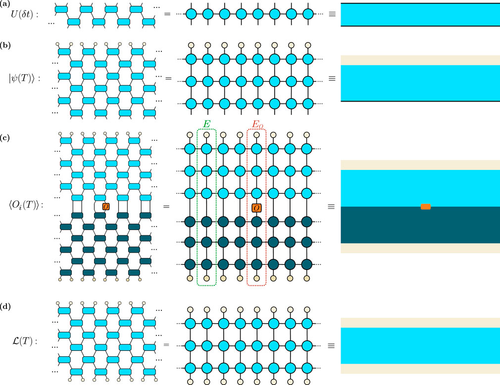
Figure 1. Time runs from top to bottom. All quantities are represented as a brick-wall circuit (left column), with matrix-product operators (center column) and in an abstract representation (right column), where the black boundaries denote open indices. (a) A graphical representation of the first-order Suzuki–Trotter decomposition of the time-evolution operator $U(\delta t)$ for a small time step $\delta t$ and for nearest-neighbor interactions. (b) $|\psi (T)\rangle ={\prod }_{i=1}^{n_T}U(\delta t)|{\psi }_0\rangle$, the Trotterized time evolution of an initial product state $|{\psi }_0\rangle$ (depicted in gray) up to time $T=n_T\cdot \delta t$. (c) $⟨O_i(T)⟩$: the time-dependent expectation value of a single body observable $⟨O_i(T)⟩=⟨{[U^{†}(\delta t)]}^{n_T}{O}_i{[U(\delta t)]}^{n_T}⟩{\psi }_0$ (darker shaded tensors refer to $U^{†}$). We have highlighted the transfer matrix $E(T)$ in green and the operator transfer matrix $E_O(T)$ in orange. (d) The Loschmidt echo $\mathcal{L}(T)=⟨{[U(\delta t)]}^{n_T}⟩{\psi }_0$.

Figure 2

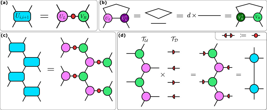
Figure 2. (a) By performing a singular value decomposition of elementary unitary gates derived from the Trotter expansion of the real-time dynamics induced by the two-qudit time-evolution operator $U_{i,i+1}=U_L\cdot \mathrm{\Sigma }\cdot V_R$. (b) shows the normalization conditions of the relevant tensors. We can define the two-dimensional tensor network (c, d) describing the dynamics and interpret the evolution in space as a sequence of unitary evolutions driven by ${\mathcal{T}}_U$ plus weak measurements driven by ${\mathcal{T}}_D$.

As a result of the discretization of the time evolution, any dynamical quantity we are interested in will be expressed in terms of numerous tensors, giving rise to a two-dimensional network that must be contracted. To give an example, the TN representing the time-dependent expectation value of a local operator acting on a few sites of the system, $⟨O(T)⟩$, is depicted in Figure 1c and written from top to bottom as follows: starting from an initial state $|{\psi }_0\rangle$, we apply $U(T)$, then the operator $O$, followed by the Hermitian conjugate of the time-evolved state, $\langle {\psi }_0|U^{†}(T)$. The latter can be seen as a part of “backward” time evolution, so that in the Keldysh formalism $|\psi (T)\rangle =U(T)|{\psi }_0\rangle$ represents the “forward” contour, while $\langle \psi (T)|$ represents the “return” contour (Hastings and Mahajan, 2015; Tirrito et al., 2018), with the operator $O$ at the middle. Another quantity of interest is the return amplitude of a time-evolved state to its initial configuration, which can be referred to as a Loschmidt echo (Figure 1d):

$\mathcal{L}\left(T\right)=⟨{\psi }_0|\psi \left(T\right)⟩=⟨{\psi }_0|U\left(T\right)|{\psi }_0⟩.(2)$

The task of contracting two-dimensional TNs is, in general, exponentially hard (Schuch et al., 2007). The traditional prescriptions of quantum mechanics typically involve a contraction row by row along the temporal axis. In this case, the complexity of the contraction is dictated by the entanglement entropy of the time-evolved $|\psi (T)\rangle$ if the contraction starts from the initial state (Verstraete and Cirac, 2006), or by the operator entanglement if the contraction involves the Heisenberg evolution of an operator (Prosen and Pižorn, 2007; Prosen and Žnidarič, 2007; Pižorn and Prosen, 2009). Due to the entanglement barrier, these entropies typically increase linearly with time, corresponding to an exponential growth of the bond dimensions involved, so generally, these contractions cannot be carried out efficiently. Yet, it is clear that another contraction direction is possible: one can, namely, start from the left and right edges of the system and perform contractions along the space direction (Bañuls et al., 2009; Hastings and Mahajan, 2015; Carignano et al., 2024). The basic building blocks involved in this “transverse” contraction are now the columns of the 2D network, which can be seen as states and operators defined at different moments of time for a fixed spatial site. We will refer to them as “temporal” MPSs and MPOs (tMPSs and tMPOs), respectively. The contraction procedure then goes as follows: starting from the edges of a system of $N$ constituents we identify a “left” tMPS $\langle L^{[1]}|$ and a “right” one $|R^{[N]}\rangle$, as well as the $j$-th column tMPO $E^{[j]}(T)$, cf. Figure 1c. At each step, we build the tMPSs,

$\langle L^{\left[k\right]}|\to \langle L^{\left[k+1\right]}|=\langle L^{\left[k\right]}|E^{\left[k+1\right]}\left(T\right),(3)$

$|R^{\left[l\right]}\rangle \to |R^{\left[l-1\right]}\rangle =E^{\left[l-1\right]}\left(T\right)|R^{\left[l\right]}\rangle ,(4)$

by applying to them the columns associated with the neighboring site. In this way, the 2D TN equals the overlap between the two tMPSs representing the transverse contraction until adjacent columns. Thus, quantities like the Loschmidt echo are given by $\mathcal{L}(T)=⟨L_{\mathcal{L}}^{[i]}|R_{\mathcal{L}}^{[i+1]}⟩$, while, for instance, the expectation value of a local observable $O$ acting on the $i$-th site reads $⟨O_i(T)⟩=\langle L^{[i-1]}|E_O^{[i]}|R^{[i+1]}\rangle$, with $E_O^{[i]}$ being the tMPO column with the insertion of the operator (see Figure 1c). Analogously to what happens for MPS defined in space, we are interested in finding the relevant quantity dictating whether an efficient representation of these transverse states is possible, for example, a “temporal” entanglement (Bañuls et al., 2009; Hastings and Mahajan, 2015; Carignano et al., 2024; Lerose et al., 2023), which can be seen as a measure of correlations of a subsystem with itself at different times. Note that while the transfer matrix evolving in time $U(\delta t)$ corresponds to a unitary operator, for the transverse contraction, the spatial evolution is governed by the non-unitary matrices $\{E^{[k]}\}$, as can be seen by the decomposition in Figures 2c, d. In this sense, the contrasting nature of the transverse evolution with respect to the usual one can give rise to different behaviors of the complexity of contracting the whole 2D TN with time, as reviewed in Section 5. More specifically, from Figure 2, we can see one step of space translation as a unitary evolution ${\mathcal{T}}_U$ plus an additional insertion of real diagonal matrices ${\mathcal{T}}_D$ containing singular values. After proper normalization, these operations can be related to weak measurements (Ippoliti and Khemani, 2021).

Depending on the network structure associated with the desired dynamical quantity, further operations can be performed to carry out the transverse contraction in a more efficient way. In particular, if we are interested in computing the time evolution of the expectation values of a local operator or few-body correlators, it should be noticed that working out a transverse contraction may induce correlations between the forward and return contours if there is information partially traced out (see Figure 3a for a sketch). These correlations are long-ranged by default as a consequence of the setup, which makes the tMPS representation impractical. To overcome this problem, “folding” the network so that both contours are merged via a vectorization operation has been proposed (Bañuls et al., 2009): $\langle \psi (T)|O|\psi (T)\rangle =\langle \phi |(\mathbb{I}\otimes O)|\psi (T)\rangle \otimes |\bar{\psi }(T)\rangle$, where $|\bar{\psi }(T)\rangle$ is the complex conjugate of $|\psi (T)\rangle$, and the vector $|\phi \rangle ={\otimes }_{k=1}^N\left({\sum }_{i_k=1}^d|i_k\rangle \otimes |i_k\rangle \right)$ is introduced to reproduce the contraction between the forward and return contours. In this manner, the transverse contraction of the folded network can lead to tMPSs with a drastically reduced temporal entanglement, allowing for an advantage compared to standard methods (see Figure 3b).

Figure 3

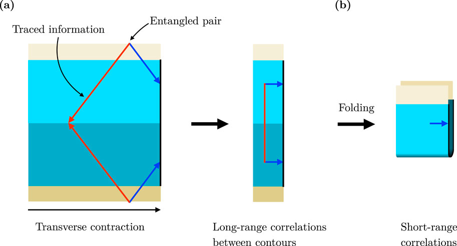
Figure 3. For a setup including both forwards and backwards time evolution (cfr. Figure 1c), we show in (a) Graphical representation of how the correlations between contours are formed for a local entangled pair that propagates freely in opposite directions. The excitation marked in red remains in the contracted subsystem throughout the entire evolution so that it is traced in the transverse contraction. On the other hand, the excitation marked in blue leaves the subsystem and enters into the complement. Due to the spatial entanglement between the red and blue excitations, the transverse contraction leads to correlations between contours. (b) The associated long-range correlations are converted into short-range correlations through the folding operation.

Aside from providing a novel way to possibly circumvent the entanglement barrier, the idea of a transverse contraction can provide a natural bridge towards the formalism of open quantum systems and, more specifically, to the idea of an influence functional. To see this, let us recall that within the path integral formulation of quantum mechanics, open quantum systems can be studied by constructing the path integral of the system plus environment and, subsequently, integrating out the degrees of freedom of the latter. The result of this integration is what is called an influence functional (IF), corresponding to a function of the time-trajectories of the system.

The IF encodes the effects of the environment on the system and allows evolving the latter’s reduced density matrix. Being a function of time-dependent coordinates, the IF can be treated as a vector of the multi-time Hilbert space of the system (Petrat and Tumulka, 2014) and represented using a temporal MPS (Lerose et al., 2021a). In the context of our TN representation, the equivalence between the two becomes clear if we now observe that in the transverse contraction, we effectively trace out the degrees of freedom of a part of the many-body system (i.e., the environment), precisely encoding their influence on the rest (the system of interest) at different times through the resulting tMPSs. The folding operation provides another step in this direction, as its overlapping forward and backward time-evolution paths reproduce precisely the Schwinger–Keldysh contour, which is typically encoded in the IF construction.

Having established such a connection, one can leverage the powerful machinery of tensor networks to provide an efficient representation of these functionals encoding the dynamical properties of the system (Lerose et al., 2021a; Giudice et al., 2022; Lerose et al., 2023). We will elaborate further on this encoding in the following sections after introducing the relation of these objects with the process tensors.

3 The connection between process tensors and influence functionals

Process tensors, which we will define properly in the following, were originally introduced as a generalization of channels for operators. They were “introduced as a tool to optimize quantum circuit over a set of unknown gates for a given task” (Chiribella et al., 2008; Chiribella et al., 2009). They can also be connected with the idea of multiple-time states (Aharonov et al., 2007; Leifer, 2006; Leifer and Spekkens, 2013) discussed in the context of quantum foundations. In this section, we will introduce the concept of the process tensor, following the presentations of Dowling et al. (2024), Pollock et al. (2018), and Pollock (2018), and relate it to the tensorial objects encountered in Section 2. In the study of the evolution of open quantum systems, a significant challenge is that of generalizing the notion of Markovianity of classical stochastic processes (Pollock et al., 2018). A classical stochastic process is defined by the joint probability distribution of a stochastic variable $X$ that describes the state of the system at several instants of time, $P_c(X_n,t_n;X_{n-1},t_{n-1};\cdots ;X_1,t_1)$. Markovianity implies that the state of the system at a given time only depends on its state at the immediately previous time,

$P_c\left(X_n,t_n;\cdots ;X_1,t_1\right)=P_c\left(X_n,t_n;X_{n-1},t_{n-1}\right).(5)$

The generalization of these ideas to the quantum realm is not straightforward because the measurements needed to determine the control parameters X will disturb the process that we want to characterize. The multi-time process tensor formalism overcomes this problem by establishing a clear separation between the process and the control operations performed by the observer, leading to a definition of Markovianity that reduces to Equation 5 for classical processes.

The control operations are completely positive trace non-increasing actions on the system, representing, for example, a unitary transformation (trace preserving) or a possible result from a measurement (trace decreasing). These operations are often called instruments. We might be interested in a set of available instruments at an instant in time, each of them to be chosen with a given probability. We represent the set of available instruments as Kraus operators $A=\{A_j\}$ defining a quantum channel. The resulting quantum channel must also be trace non-increasing:

${\displaystyle \sum _j}{A}_j^{†}{A}_j\le \mathbb{I}.(6)$

We consider that the control operations intervene at $n$ different instants of time $t_1,\dots t_n$. The process tensor $P$ is a linear and completely positive map from the set of control operations $\mathcal{A}=\{A^{[t_1]},\dots ,A^{[t_n]}\}$ acting on an open system to output states of the system plus its environment. The output states can be sub-normalized according to the success probabilities of the chosen instruments. The process tensor thus encodes the system and environment dynamics, as well as the information on their initial state. In order to simplify notation and anticipate the discussion below, we assume that the same set of instruments is available at each instant of time, that is, $A^{[t_1]}=\cdots =A^{[t_n]}=A$. We denote a particular choice of instruments by ${\mathcal{A}}_{{\tau }_1\dots {\tau }_n}=\{A_{{\tau }_1},\dots A_{{\tau }_n}\}$. The process tensor would then map

$P:{\mathcal{A}}_{{\tau }_1\dots {\tau }_n}\to |P{\mathcal{A}}_{{\tau }_1\dots {\tau }_n}\rangle \in {\mathcal{H}}_{S\otimes E}(7)$

with

$|P{\mathcal{A}}_{{\tau }_1\dots {\tau }_n}\rangle =U\left(T,t_n\right)A_{{\tau }_n}\cdots U\left(t_2,t_1\right)A_{{\tau }_1}U\left(t_1,0\right)|{\psi }_{SE}^0\rangle ,(8)$

where $|{\psi }_{SE}^0\rangle$ is the initial state of the system plus the environment, and $U(t_i,t_{i-1})$ implements their joint unitary evolution between times $t_{i-1}$ and $t_i$. Figure 4 displays a graphical representation of Equation 8.

Figure 4

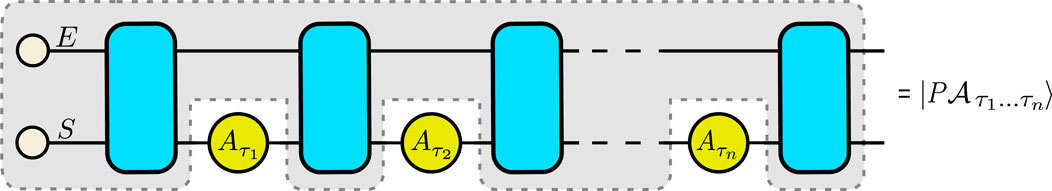
Figure 4. The process tensor is represented as the gray shadowed area, containing the information on the initial state of the system (S) and its environment (E), together with their joint evolution under the unitaries $U(t_i,t_{i-1})$. The evolution of the system is monitored by control operations ${\mathcal{A}}_{{\tau }_1\dots {\tau }_n}=\{A_{{\tau }_1},\dots ,A_{{\tau }_n}\}$ performed at times $t_1,\dots ,t_n$. The process tensor maps the chosen control operations to the output state of the system plus the environment, $|P{\mathcal{A}}_{{\tau }_1\dots ,{\tau }_n}\rangle$.

Let us proceed to show how the process tensor language naturally emerges in the study of the closed dynamics of a quantum spin chain. Imagine that we start with the simplest scenario obtained by considering the evolution of two constituents. In order to make a connection with Figure 4, we can assume that one plays the role of the system and the other of the environment. We also limit ourselves to the case of a two-times process tensor where an initial product state evolves under the unitary $U$ for one time step, then might undergo a control operation and finally evolves again for an extra step, as shown in Figure 5a. For this setup, the process tensor has four open legs: two (one “input” and one “output”) after one step of evolution, which, on the introduction of an instrument, are mapped to the temporal legs defined above, and two output legs after the second step, which are spatial legs corresponding to the two constituents. If we contract the former two legs together (corresponding to a trivial choice of instrument, $A=\mathbb{I}$), the latter will represent the final state of such constituents.

Figure 5

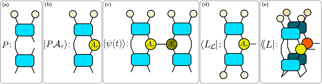
Figure 5. Tensor network representation of (a) the process tensor $P$ for two spins and two time steps and (b) the process tensor with an instrument $A_{\tau }$ applied. (c) Evolution of a four-spin system where, according to Equation 12, the central cyan gate is interpreted in terms of instruments applied to the associated left and right process tensors. (d) The left temporal vector in the context of a Loschmidt echo represented as the overlap of the spatiotemporal state $|P{\mathcal{A}\rangle }_L$ Equation 13 on the initial state of the spins. The open leg corresponds to the promotion of the instrument labels to elements of a temporal Hilbert space ${\mathcal{H}}_T$. (e) The partial trace of $|P{\mathcal{A}\rangle }_L$ over its spatial degrees of freedom gives rise to the influence functional of the two left spins.

Among the possible choices of instrument sets, one is relevant for the connection we want to make here: it consists of using as instruments the rows (columns) of the left (right) unitary emerging from the decomposition of the evolution operator shown in Figure 2a, $U=U_L\mathrm{\Sigma }{V}_R$. Namely, we can choose a set $A=\{A_{\tau }\}$ such that

${\left[A_{\tau }\right]}_{\alpha \beta }=\frac{1}{\sqrt{d}}{\left[U_L\right]}_{\alpha \beta ;\tau },(9)$

with $\tau =1,..,d^2$. The normalization $1/\sqrt{d}$ renders the quantum channel defined by $A$ trace preserving (see Figure 2b)

${\displaystyle \sum _{\tau =1}^d}{\left[A_{\tau }^{†}{A}_{\tau }\right]}_{\alpha \gamma }=\frac{1}{d}{\displaystyle \sum _{\tau ,\beta }}{\left[U_L^{*}\right]}_{\beta \alpha ;\tau }{\left[U_L\right]}_{\beta \gamma ;\tau }={\delta }_{\alpha \gamma }.(10)$

The set $A$ so defined assigns equal probability to each instrument. Although a valid choice, this, however, does not represent the probabilities with which the $A_{\tau }$ are selected as the system evolves. That information is encoded in the singular values ${\sigma }_{\tau }$, contained in the diagonal matrix $\mathrm{\Sigma }$. Because $U$ is unitary, we have $\sum {\sigma }_{\tau }^2=d^2$, and hence, each singular value satisfies ${\sigma }_{\tau }/d\le 1$. We can use this fact to rescale the instruments as

$A_{\tau }\to \sqrt{\frac{{\sigma }_{\tau }}{d}}{A}_{\tau },(11)$

Such that now $A$ will describe, in general, a trace decreasing quantum channel. We denote as $A_{\tau }^{\prime }$ the alternative set of instruments associated with the right unitary $V_R$. In this way, the decomposition of the two-body gates can be rewritten as

$U=d^2{\displaystyle \sum _{\tau }}{A}_{\tau }{A}_{\tau }^{\prime }.(12)$

This specific choice of instruments leads us to the first connection between the multi-time process tensor and the influence functionals. To see this, let us now consider a system of four qudits evolving under a brick-wall circuit based on the same two-body gates as before. Splitting the system in half, we consider that the left and right qudits undergo two evolution steps as before, but now the central left and right qudits are connected by one further step. We can interpret such step as the insertion of the instruments $A_{\tau }$ and $A_{\tau }^{\prime }$ introduced above on the left and right process tensors, defined as in Figure 5a. This is shown in Figure 5d, where a sum over instruments is understood. We make a step further and associate the labels of the instruments with elements of a “temporal” Hilbert space: $\tau \to |\tau \rangle \in {\mathcal{H}}_T$. This allows us to define spatiotemporal states in the enlarged Hilbert spaces ${\mathbb{C}}^d\otimes {\mathbb{C}}^d\otimes {\mathcal{H}}_T$ and ${\mathbb{C}}^d\otimes {\mathbb{C}}^d\otimes {\mathcal{H}}_T^{*}$ as follows:

$|P{\mathcal{A}\rangle }_R={\displaystyle \sum _{\tau }}|P{A}_{\tau }^{\prime }\rangle |\tau \rangle ,|P{\mathcal{A}\rangle }_L={\displaystyle \sum _{\tau }}|P{A}_{\tau }\rangle \langle \tau |.(13)$

Recall that both the left and right process tensors and the instrument sets $\mathcal{A}$ and ${\mathcal{A}}^{\prime }$ are constructed out of the same object, the two-body evolution gate $U$. Hence, the same information is contained in the process tensors and the spatiotemporal states (Equation 13), particularly when it comes to the computational complexity of encoding these objects, and in this sense, we can use them interchangeably.

Suppose we are interested in the Loschmidt echo, Equation 2, of the four spins, which, according to the results of Section 2, can be computed as the overlap of left and right temporal vectors $⟨L_{\mathcal{L}}|R_{\mathcal{L}}⟩$. Following the discussion above, the left temporal vector is obtained by projecting the space-like degrees of freedom of $|P{\mathcal{A}\rangle }_L$ onto their initial state,

$\langle L_{\mathcal{L}}|=d{⟨{\psi }_{0L}|P\mathcal{A}⟩}_L.(14)$

We are assuming that the initial state of the four spins is a product state, such that we can assign a well-defined initial state to the left two spins, $|{\psi }_{0L}\rangle$. This equivalence is represented in Figure 5c. Following an analogous reasoning, we can identify a right process tensor and the corresponding temporal vector as $|R_{\mathcal{L}}\rangle =d{⟨{\psi }_{0R}|P\mathcal{A}⟩}_R$.

We turn now to the network associated with another typical dynamical quantity of interest, namely, the expectation value of an operator. Focusing on the left half of our four-spin system, this network will contain both $|P{\mathcal{A}\rangle }_L$ and its conjugate $\langle P\mathcal{A}{|}_L$, which can be associated with the description of backward time evolution. The trivial case of an identity operator in the system + environment legs immediately leads to a partial trace obtained by multiplying the two process tensors over their open spatial indices, as illustrated in Figure 5e. Of course, the result can be generalized with the inclusion of different operators inserted in the spatial legs of the process tensors, leading to the same structure. The resulting object, describing time evolution on a time contour involving both forward and backward evolution, is precisely the influence functional of the left half of the system, as introduced in Section 2. In the language of process tensors, this left influence functional can thus be seen as the reduced density matrix of $|P{\mathcal{A}\rangle }_L$ traced over its spatial degrees of freedom:

${\rho }_T^L=d^2{{\mathrm{t}\mathrm{r}}_{\text{space}}}_L\left|P\mathcal{A}\right.⟩{\left.⟨P\mathcal{A}\right|}_L.(15)$

If we vectorize ${\rho }_T^L$ by “folding” the network and joining the temporal legs associated with the forward and backward evolution, we can interpret it as a state $\langle \langle L|$, as shown in Figure 5e.

At this point, it is straightforward to extend these quantities to the many-body setting considered in Section 2. We start by considering the tensor network that describes the evolution of the system under $N$ Trotter steps. We focus on the partial contraction of such a network on a spatiotemporal patch, such as the left half of the system. The resulting tensor has spatial and temporal open legs represented by horizontal and vertical black solid lines in Figure 6a. We divide its spatial legs into the system and environment, such that the system comprises only the rightmost spin of the left patch. In analogy with (13), we can interpret this spatiotemporal tensor in the language of process tensors by defining

$|P{\mathcal{A}\rangle }_L={\displaystyle \sum _{{\tau }_1\dots {\tau }_n}}|P{\mathcal{A}}_{{\tau }_1\dots {\tau }_n}\rangle \langle {\tau }_1\dots {\tau }_n|,(16)$

where $P$ is a generalization of Figure 5a, and the instruments are derived again from the singular value decomposition of the 2-qubit evolution gate. If we now project the spatial legs of $|P{\mathcal{A}\rangle }_L$ onto the initial state of the chosen spatial patch, we obtain the left environment defined in the context of Loschmidt echoes as described in Equation 14 and illustrated in Figure 6b.

Figure 6

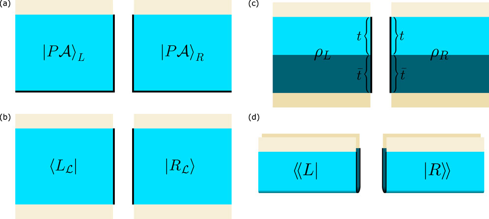
Figure 6. (a) Contracting a patch of the spatiotemporal tensor network gives rise to a tensor with both spatial and temporal open legs, represented by black solid lines. When cutting the network, we split the two-body gates joining the left and the right halves following the recipe of Figure 2. The resulting tensor can be identified with the spatiotemporal state $|P{\mathcal{A}\rangle }_L$ defined in (13), with the choice of instruments (11). (b) Starting from a product state, we consider the overlap of $|P{\mathcal{A}\rangle }_L$ with the initial state of the left half of the system, obtaining the left temporal state defined in the context of Loschmidt echo, $\langle L_{\mathcal{L}}|$. (c) The partial trace of $|P{\mathcal{A}\rangle }_L$ on its spatial degrees of freedom gives rise to the left influence functional defined in standard tensor networks studies of the dynamics. (d) We can vectorize and fold the influence functional, obtaining the state $\langle \langle L|$. The same constructions hold for the right half of the tensor network.

In the same way, the left influence functional associated with the calculation of local observables is also obtained from Equation 15 in the many-body setting. Figures 6c, d display the standard and folded versions of the influence functionals.

In the above formulas, we have made clear that the influence functional is, in general, a mixed state. If one is interested in the compressibility of such a mixed state in terms of the matrix-product operator, one must consider the operator entanglement of the influence functional, that is, the entanglement entropy of its vectorized form that we have indicated with $\langle \langle L|$.

In the following section, we will discuss some of the algorithms developed for efficient compression of the influence functional as temporal MPS and the complexity of such an encoding.

4 Algorithms for obtaining a tensor network encoding of the influence functional, dissipative time evolutions

The transverse contraction framework introduced in Section 2 for the description of the dynamics of quantum many-body systems opens the way to an efficient encoding of process tensors and influence functionals in the compact form of temporal MPS. The best procedure to contract the network associated with time evolution can vary depending on the system we are considering and the truncation procedure we choose, as described in the following. For a finite chain, one possibility is to start from the sides, identify the left- and rightmost columns as temporal MPS, and progressively apply columns of tMPO to them until reaching the center, truncating at each step to prevent their bond dimension from growing exponentially. Alternatively, for an infinite homogeneous system, one could start growing the system from the center in the spirit of the infinite version of the density matrix renormalization group (DMRG) algorithm.

In this section, we explain the main aspects to take into account for these transverse algorithms and the compression procedure for these tMPSs. The steps described here can be applied to both pure and mixed states, corresponding to the “folded” picture introduced in Section 2. As such, in the following description whenever possible we will consider generic left vectors $\langle L|$ (the same goes for $|R\rangle$), assuming that—depending on the case considered—they refer to the Loschmidt echo-type setup $\langle L_{\mathcal{L}}|$ or the vectorized density matrices $\langle \langle L|$ introduced above.

4.1 Cost functions used for compressing tMPSs

Transverse contraction algorithms rely on the successive applications of tMPOs to the tMPSs associated with the left and right halves of the system, which we will refer to as $\langle L|$ and $|R\rangle$, respectively, with subsequent recompression that can be performed following different criteria.

For this iterative process, the simplest prescription would be to compress both $\langle L|$ and $|R\rangle$ separately, following the standard recipe in MPS literature, through their corresponding reduced density matrices (RDM) (Bañuls et al., 2009): for any time $t\in [0,T]$ ($T$ being the total time of the evolution) appearing in the Trotterized network, one can define a bipartition in two temporal intervals $A=[0,t]$ and $B=[t+\delta t,T]$ and build

${\rho }_A^L\left(t\right)={\mathrm{t}\mathrm{r}}_B\left|L\right.⟩\left.⟨L\right|,{\rho }_B^L\left(t\right)={\mathrm{t}\mathrm{r}}_A\left|L\right.⟩\left.⟨L\right|.(17)$

and the same for ${\rho }_{A,B}^R$. From these, we can compute the standard entanglement entropies,

${\mathcal{S}}_{\alpha }\left({\rho }_A\right)=\frac{1}{1-\alpha }\log \left[{\mathrm{t}\mathrm{r}}_A{\left({\rho }_A\right)}^{\alpha }\right],(18)$

where $0\le \alpha \le \infty$ is the Rényi parameter. As is well known, for this prescription based on RDMs, the complexity of constructing $\langle L|$ and $|R\rangle$ can be related to these $S({\rho }_A)$, which we refer to as temporal entanglement entropies.

However, the transverse contraction framework offers more possibilities when it comes to the optimization of the left and right vectors. The first insight in this direction was presented in Hastings and Mahajan (2015), where it was realized that the imaginary time-evolution equations for the RDM of the right vector² can be rephrased as a DMRG algorithm for a system mirrored across the bipartition, with a slightly modified Hamiltonian. This can be intuitively seen by relating the (temporal) RDM $\left|R\right.⟩\left.⟨R\right|$ to the evolution of a system made of two copies of the right subsystem, where one follows the same equations as the other, up to a complex conjugation. In turn, this inspired the introduction of a modified cost function, built from the right vector and its transpose: ${\tilde{\rho }}_R\propto \left|R\right.⟩\left.⟨\bar{R}\right|$ (where the complex conjugation is performed to “undo” the conjugation of the bra). An optimization with respect to this object provided a good estimate for the whole left-right contraction of the network. As a matter of fact, for a system with reflection symmetry, $\langle \bar{R}|$ coincides with the left vector $\langle L|$. This observation then motivates us to focus directly on optimizing the overlap $⟨L|R⟩$, by providing a faithful representation of the reduced transition matrices (RTM), which for an arbitrary bipartition $A-B$ reads

${\tau }_A\left(t\right)={\mathrm{t}\mathrm{r}}_B\frac{|R\rangle \langle L|}{⟨L|R⟩},(19)$

and analogously for ${\tau }_B(t)$. Following this intuition, the complexity of performing the network contraction should be related to the properties of the RTM (Equation 19) rather than the RDMs defined in Equation 17. In Figure 7, we show a graphical representation of these quantities, comparing the RTMs built for the Loschmidt echo and the (folded) IF with the regular RDM.

Figure 7

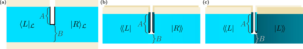
Figure 7. (a) Reduced transition matrices used to compute the generalized temporal entropies from the path integral encoding a Loschmidt echo. (b) Reduced transition matrices used to compute the generalized temporal entropy in the context of a quantum quench. Notice that they encode partial overlap of the left and right influence functional in that context. (c) Shows the temporal entanglement defined as the entanglement of the vectorized left (or right) influence functional. Notice that when there is a reflection symmetry, (c) differs from (b) because it requires considering a transposition of the right influence functional before taking the partial overlap. Also, given that we are using the vectorized version of the influence functional, its entanglement actually represents the operator entanglement of the influence functional, which is the relevant version if we are interested in understanding how much we can compress the influence functional as an MPO.

An extended notion of entropy based upon the RTMs can be defined by substituting ${\rho }_{L,R}(t)$ by $\tau (t)$ in Equation 18, resulting in the generalized entanglement and Rényi entropies (Nakata et al., 2021; Doi et al., 2023). The relevant quantities for the evaluation of such generalized entropies are the eigenvalues of the RTM, which are not necessarily positive or even real. Consequently, the generalized entropies are complex-valued quantities.

The relationship of these interesting new quantities with the complexity of representing the associated tensor network is still the object of investigation (Hastings and Mahajan, 2015; Carignano et al., 2024; Carignano and Tagliacozzo, 2024). In fact, the compression procedure based upon RTMs is not straightforward: unlike the (reduced) DMs, $\tau (t)$ is a non-Hermitian matrix. As such, eigenvalues and singular values do not coincide in general, and it is not a priori clear which of them is used as a guideline for the network compression. In the following, we will use the singular values as cost functions for truncation as they provide a well-defined set of positive and real quantities. It is also relevant to discuss the role of gauge freedom in these non-Hermitian problems. In principle, given a transfer matrix $E(T)$, one can perform a gauge transformation $E(T)\to \mathcal{X}E(T){\mathcal{X}}^{-1}$ such that the 2D tensor network associated with the time evolution remains invariant. It has been observed (Tang et al., 2025) that the temporal entanglement in the $\langle L|$ and $|R\rangle$ can be arbitrarily reduced by these transformations. However, this comes at the cost of accuracy because these transformations can shift the relevant contributions to the overlap $⟨L|R⟩$ to the tails of singular values, which are truncated in the required compression procedure. This issue is mitigated when considering reduced transition matrices, as these gauge transformations are canceled when computing these objects.

As such, we will focus on this type of truncation here while recalling that other methods based on bi-orthogonalization techniques can also be used when dealing with non-Hermitian transfer matrices (Wang and Xiang, 1997; Xiang, 1998; Zhong et al., 2024).

4.2 Compression procedure

The compression of the tMPS is carried out by constructing the desired cost function, such as the RDM (Bañuls et al., 2009) or the RTM (Hastings and Mahajan, 2015; Carignano et al., 2024), and approximating it to a given rank for every possible bipartition. This is commonly achieved through singular value decompositions of the relevant objects.

While the truncation over RDM is amply covered in standard TN literature, let us briefly review the procedure for the case of an RTM. The notation used is as follows (see Figures 8a, b): given a tMPS, we will use Greek letters for the physical indices and Latin letters for the bond ones. In addition, given the bipartition introduced above, we define the matrices ${\mathrm{\Lambda }}_A(t)$, which result from the contraction of the subsystem $A$ of $\langle L|$ with the one of $|R\rangle$, and ${\mathrm{\Lambda }}_B(t)$ as the counterpart for the subsystem $B$. Notice that ${\mathrm{\Lambda }}_A(t)$ and ${\mathrm{\Lambda }}_B(t)$ can be seen as acting at the bond level, namely, ${\mathrm{\Lambda }}_{A,B}(t)\equiv {({\mathrm{\Lambda }}_{A,B}(t))}_{i_t{i}_t^{\prime }}$.

Figure 8

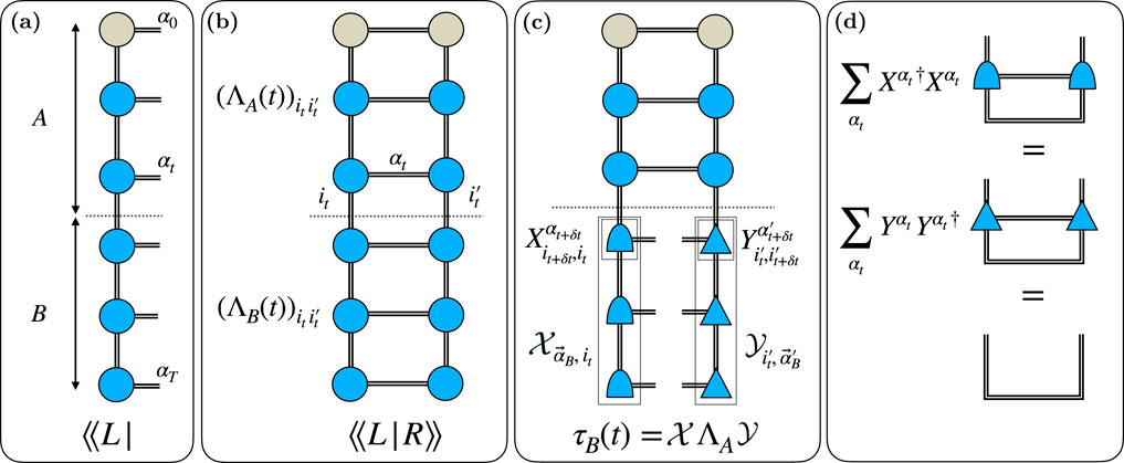
Figure 8. Pictorial notation for the compression procedure assuming folded tMPSs. (a) Bipartition of a tMPS into top and bottom subsystems. (b) Definition of ${\mathrm{\Lambda }}_A(t)$ and ${\mathrm{\Lambda }}_B(t)$. (c) Reduced transition matrix ${\tau }_B(t)$ once the bottom subsystems of $\langle L|$ and $|R\rangle$ are brought into canonical form, that is, they are expressed in terms of left-normalized $\{X^{{\alpha }_k}\}$ and right-normalized $\{Y^{{\alpha }_k}\}$ matrices, respectively. (d) By definition, the matrices $\{X^{{\alpha }_k}\}$ and $\{Y^{{\alpha }_k}\}$ satisfy the condition ${\sum }_{{\alpha }_k}{X}^{{\alpha }_k†}{X}^{{\alpha }_k}={\sum }_{{\alpha }_k}{Y}^{{\alpha }_k}{Y}^{{\alpha }_k†}=\mathbb{I}$, from which it follows that ${\mathcal{X}}^{†}\mathcal{X}=\mathcal{Y}{\mathcal{Y}}^{†}=\mathbb{I}$.

With these definitions, we now proceed to explain the compression procedure. This is done by truncating the RTMs (Equation 19) associated with the different bipartitions, which are consecutively obtained by tracing the temporal sites from the $t=0$ to $t=T$, or the other way around. For the sake of concreteness, let us assume the former possibility, although we discuss the relevance of this choice at the end of the section. Thus, we start by cutting the tMPS at the first bond index from $t=0$ and bringing the $B$ subsystems of both $\langle L|$ and $|R\rangle$ into canonical form, namely, writing them in terms of left-normalized $\{X^{{\alpha }_k}\}$ and right-normalized $\{Y^{{\alpha }_k}\}$ matrices, respectively, as depicted in Figures 8c, d. Once this is done, ${\tau }_B(t)$ reads

${\tau }_B\left(t\right)=\mathcal{X}{\mathrm{\Lambda }}_A\left(t\right)\mathcal{Y},(20)$

where $\mathcal{X}$ $(\mathcal{Y})$ represents the left (right) isometry coming from contracting the $\{X^{{\alpha }_k}\}$ $(\{Y^{{\alpha }_k}\})$ matrices (see Figure 8c).

Given that $\mathcal{X}$ and $\mathcal{Y}$ are left and right isometries, respectively, ${\tau }_B(t)$ and ${\mathrm{\Lambda }}_A(t)$ have the same singular values, so that by means of the gauge freedom of the tMPSs, the optimization problem has been reduced to applying an SVD to ${\mathrm{\Lambda }}_A(t)$ and discarding the smallest singular values, instead of decomposing the exponentially large matrix ${\tau }_B(t)$. The compressed tMPSs are obtained by inserting the associated projectors on the link that specifies the bipartition. Furthermore, a subsequent gauge transformation can be performed on the updated tensors to guarantee that ${\mathrm{\Lambda }}_A(t)$ reduces to an identity. Once optimized the first link, we must only update ${\mathrm{\Lambda }}_t$ by tracing out the adjacent site

${\mathrm{\Lambda }}_A\left(t+\delta t\right)={\displaystyle \sum _{{\alpha }_t}}{X}^{{\alpha }_t}{\mathrm{\Lambda }}_A\left(t\right)Y^{{\alpha }_t},(21)$

and repeat the process until all the bonds are truncated.

It should be noted that, depending on which dynamical quantity we are interested in as well as the cost function used, a meaningful truncation can require starting from $t=0$ or $t=T$. This is especially the case if one compresses the left and right tMPSs for influence functionals through their RTM (Equation 19) in the folded network. As an example, if one follows Hastings and Mahajan (2015), the compression must be carried out from $t=0$ to $t=T$: as the RTM constitutes a 2D TN that does not include any local operator $O$, the contraction of $B(t)$ represents the multiplication of the time-evolution operator with its adjoint, which gives the identity (see Figure 9a). Due to this trivialization, if one performs a truncation starting from $t=T$, the states $\langle L|$ and $|R\rangle$ after the compression would have a bond dimension of 1 and contain no useful information for further calculations. When starting from $t=T$, this simplification can be avoided by including $O$ in the definition of the RTM, as proposed by Carignano et al. (2024). This is done by contracting the associated transfer matrix $E_O$ with either $\langle \langle L|$ or $|R\rangle \rangle$, such that the resulting tMPSs are denoted by $\langle \langle L_O|$ and $|R_O\rangle \rangle$, respectively. Assuming that the operator $O$ is included in $|R\rangle \rangle$, we can define the RTM

${\tau }_A^O\left(t\right)=\frac{{\text{tr}}_B|R_O\rangle \rangle \langle \langle L|}{\langle ⟨L|R_O⟩\rangle }.(22)$

Figure 9

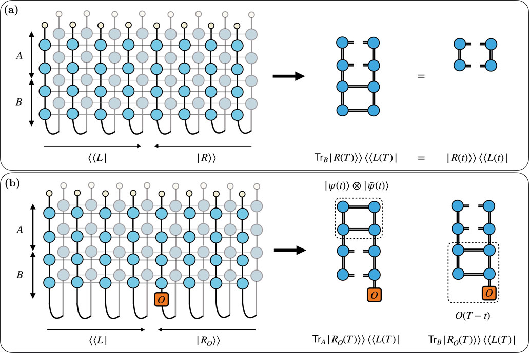
Figure 9. Two-dimensional TN representing the RTMs Equations 19, 22. (a) In case of not including the operator, the partial contraction from t to T gives $U^{†}(T-t)U(T-t)=\mathbb{I}$, so that the RTM ${\text{Tr}}_B|R(T)\rangle \rangle \langle \langle L(T)|$ equals the projector $|R(t)\rangle \rangle \langle \langle L(t)|$. Because of this simplification, the associated ${\mathrm{\Lambda }}_B(t)$ has only one non-zero singular value. Hence, the compressed tMPSs have a bond dimension of 1 when starting from the bottom side. (b) If the operator is added, then there is a clear connection with the evolution of either the state or operator depending on whether the partial contraction is done from the top or bottom, respectively.

By following this prescription, the contraction of the bottom rows gives the Heisenberg evolution $O(T-t)=U^{†}(T-t)OU(T-t)$ instead, which does not simplify (see Figure 9b). In fact, as we explain in Section 5.1, including the operator in the RTM allows for establishing a neat picture of the complexity of computing time-evolved expectation values based on the concept of operator entanglement.

This extra care concerning the directionality of the compression is a consequence of having both forward and return contours merged through the folding operation. For this reason, quantities with only the forward contour, such as the Loschmidt echo, do not present this problem. Indeed, for the Loschmidt echo starting from either the $t=0$ or $t=T$ can be seen as compressing from the side of a state evolving forwards or backward in time, respectively.

5 On the complexity of process tensors and of the influence functional

Having elucidated the connection between temporal MPS, influence functionals, and process tensors, we can now employ the techniques described in the previous section in order to complete the picture of the cost of encoding influence functionals as tensor networks, filling some of the gaps in the current understanding of their complexity. We begin by recalling some results on tMPS complexity in the literature and then discuss their implications for process tensors.

5.1 Tensor network results based on generalized temporal entanglement

As discussed in Section 4, in the framework of transverse contractions, the generalized temporal entropy can be seen as a measure describing the complexity of a faithful description of the network contraction using tMPSs.

5.1.1 Expectation values of local operators

A first result on the complexity of the tMPS associated with the time evolution of the expectation value of a local operator was given by Carignano et al. (2024). As explained in Section 4.2, one can define folded tMPSs with the insertion of the operator $O$ so that the complexity of calculating $⟨O(T)⟩$ is given in terms of the ranks of the RTMs Equation 22. Depending on whether the RTM is obtained by tracing the top or bottom subsystems, we explicitly construct the vectorized time-evolved density matrix of the initial state, $|\psi (t)\rangle \otimes |\bar{\psi }(t)\rangle \equiv {\mathrm{\Lambda }}_A(t)$ or the evolved operator $O(T-t)\equiv {\mathrm{\Lambda }}_B^O(t)$, respectively (see Figure 9b), a fact that can be used to determine the behavior of the ranks with time.

This is especially true for ${\tau }_A^O(t)$, which can be expressed as the multiplication of ${\mathrm{\Lambda }}_B^O(t)$ with the $A$-subsystems of $\langle \langle L|$ and $|R_O\rangle \rangle$, as illustrated in Figure 9b. The $A$-subsystems of the vectorized influence functionals can be described in terms of ${({\bar{\mathrm{\Lambda }}}_A^{L,R}(t))}^{1/2}$, where ${\bar{\mathrm{\Lambda }}}_A^{L,R}(t)$ are the analogies of ${\mathrm{\Lambda }}_A(t)$ for the networks $⟨⟨L|L⟩⟩$ and $⟨⟨R_O|R_O⟩⟩$, respectively; see Carignano et al. (2024) for details. Notice that the matrices ${\bar{\mathrm{\Lambda }}}_A^{L,R}(t)$ carry only information on the evolution of the state. Indeed, if we further assume reflection-invariant systems, we have ${\bar{\mathrm{\Lambda }}}_A^L(t)={\bar{\mathrm{\Lambda }}}_A^R(t)$. We thus have

$\mathcal{R}\left({\tau }_A^O\left(t\right)\right)\le \min \left\{\mathcal{R}\left({\mathrm{\Lambda }}_B^O\left(t\right)\right),\mathcal{R}\left({\bar{\mathrm{\Lambda }}}_A^L\left(t\right)\right)\right\},(23)$

where $\mathcal{R}$ stands for the rank of the corresponding matrix.

Because the rank of ${\mathrm{\Lambda }}_B^O(t)$ is dictated by its operator entanglement, we obtain that the latter provides an upper bound to the computational complexity of the transition matrices. If its growth is slower (i.e., sub-volume law) than that of the entanglement of the time-evolved state, this implies that the transverse contraction can provide a more efficient compression of the TN associated with the expectation value, a property that can be exploited numerically by truncating the tMPS starting from the operator side (Carignano et al., 2024). Explicitly, if $\mathcal{R}\left({\mathrm{\Lambda }}_B^O(t)\right)$ only increases polynomially with $T$, we have

$\mathcal{R}\left({\mathrm{\Lambda }}_B^O\left(t\right)\right)\le t^{\alpha }\Rightarrow \mathcal{R}\left({\tau }_A^O\left(t\right)\right)\le T^{\alpha }\forall t.(24)$

On the other hand, in the case of ergodic dynamics, one expects that the operator entanglement grows linearly with time (Prosen and Pižorn, 2007), implying an exponential cost in representing faithfully the IF for this problem. This was confirmed by Carignano et al. (2024), where some of the specific cases considered were found to saturate this bound.

5.1.2 Loschmidt echo

The transverse contraction framework also allows providing an analytical estimate of the computational complexity of evaluating the TN associated with the Loschmidt echo $⟨{\psi }_0|\psi (T)⟩$ for an infinite system after a global quench at a critical point, as shown by Carignano and Tagliacozzo (2024). This result was obtained by exploiting the universal properties of the model at criticality and deriving the corresponding properties from the underlying conformal field theory (CFT). The relevant object for a translation-invariant system is the (non-Hermitian) transfer matrix $E^{\mathcal{L}}(T)$ (cfr. Section 2) associated with spatial translations in the system³ and its dominant left and right eigenvectors, which can be represented as tMPSs.

The connection in the continuum limit was made again thanks to the path integral formulation, which maps the quench geometry to that of an infinite strip. CFT can then provide all the relevant information on the spectrum of the transfer matrix along the strip, as well as the generalized temporal entropy associated with a time-like cut, which can be mapped back to the reduced transition matrices $\tau (t)$. In particular, it was shown that for a quench to the critical point, the generalized temporal entropy grows like $S\sim c\log (T)$, with $c$ being the CFT central charge. This logarithmic growth at criticality (and thus the simulability of the corresponding transition matrix) and the related closing of the gap in the spectrum bear a strong resemblance to what happens in the ground states of critical chains and the corresponding spatial entanglement. In those cases, the opening of the gap as we move away from the critical point should imply that away from criticality, the generalized temporal entropies for the Loschmidt echo follow an area law, guaranteeing an even more efficient simulability using tMPSs. This is indeed the case, as confirmed by numerical simulations by Carignano and Tagliacozzo (2024). Complementing those observations, in Figure 10, we plot the maximum value of the Rényi 2 entanglement entropies for the Loschmidt echo at the critical point and close to it, showing the area and logarithmic growths expected.

Figure 10

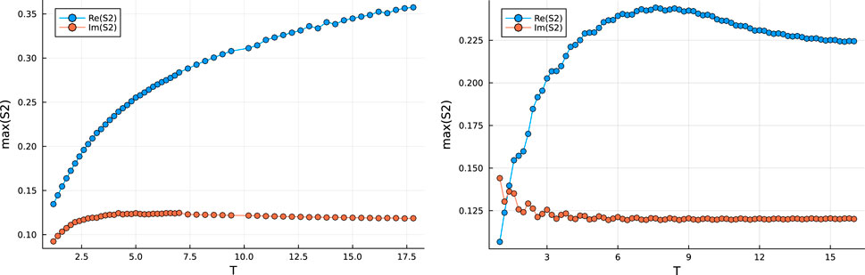
Figure 10. Examples of generalized second Rényi temporal entropies $(S2)$ built from the reduced transition matrix for the Loschmidt echo for the Ising model in a transverse field. We consider a spatially infinite system and plot the maximum of both real and imaginary parts of $S2$ as a function of time. Left: results at the critical point, where we observe a logarithmic growth. Right: away from the critical point, the entropies saturate, exhibiting an area law behavior.

5.2 Connections with other approaches

It should now be clear that one of the reasons the tensor network community has considered influence functionals and their complexity—measured in terms of temporal entropy—is the hope that these objects might be easier to encode than the evolution of states and operators, which are generally exponentially difficult to compress as simple tensor networks.

Recently, we have proposed using generalized temporal entanglement, computed from the path integral of the expectation value of local operators, as a measure of the cost of simulating these expectation values (Carignano et al., 2024). Prior studies have instead analyzed the entanglement of independent influence functionals $\langle L|$ and $|R\rangle$ or the process tensors.

Numerical observations (Bañuls et al., 2009; Frías-Pérez and Bañuls, 2022) have shown that the temporal entanglement of the influence functional $\langle L|$ grows logarithmically in some models and linearly in time for others. Subsequent studies (Sonner et al., 2021; Lerose et al., 2021b; Lerose et al., 2021c; Giudice et al., 2022; Lerose et al., 2023) confirmed these findings, associating logarithmic growth with integrability and linear growth with generic dynamics. In Hastings and Mahajan (2015), a direct connection was established between the spatial entanglement of a suitably modified model and temporal entanglement, showing that linear growth in time arises from a non-Hermitian link in the modified model’s dynamics, where energy is continually injected. These results were further validated through explicit calculations in random and dual-unitary circuits (Foligno et al., 2023; Yao and Claeys, 2024), where linear growth was found to be the generic behavior of temporal entropy for the influence functional.

Some authors have suggested that space–time duality might help overcome the entanglement barrier (Lerose et al., 2023). The evidence gathered here, however, points to the contrary: for ergodic systems, influence functionals seem to be exponentially difficult to compress using temporal matrix-product states (MPSs). This may seem counterintuitive as ergodic systems observed locally are expected to exhibit Markovian dynamics with little or no memory effects. Consequently, one might expect that the quantum channel governing the evolution of a local operator could be encoded using a temporal MPS with a small bond dimension, naturally leading to the exponential decay of correlations in time. However, we will review why this is not the case.

The first piece of evidence comes from Carignano et al. (2024), where it was shown that the bond dimension of a temporal MPS encoding the evolution of a local operator is upper-bounded by the bond dimension required to describe the operator’s evolution itself. Given the results in Prosen and Pižorn (2007) and subsequent works, the bond dimension necessary to describe operator evolution in the Heisenberg picture is expected to grow exponentially in time for ergodic systems. Such a growth has even been proposed as a definition of ergodicity. Consequently, the bond dimension of the temporal MPS encoding the influence functional is also bounded by an exponential function of time.

Building upon these insights, we incorporate findings from quantum information studies on the complexity of the process tensor in ergodic systems. Notably, the definitions of ergodicity and quantum chaos remain debated. Here, we adopt the operational definition introduced by Dowling et al. (2024), which generalizes the classical notion that chaotic systems exhibit extreme sensitivity to perturbations. In this framework, they define the “orthogonality of butterfly flutters,” meaning that two orthogonal choices of instruments applied to the same process tensor should produce orthogonal system-environment states. Furthermore, such orthogonality should not be rectifiable by a finite-depth unitary transformation, encapsulating the notion of information scrambling. Dowling et al. (2024) demonstrate that, under this definition, the process tensor has maximal entanglement for any space-time cut, implying that its temporal MPS representation must have an exponentially large bond dimension.

By taking the partial trace of the process tensor over its spatial degrees of freedom, we deduce that the influence functional—representing a maximally mixed state—is similarly encoded by an MPO with an exponentially large bond dimension. Additionally, the fully scrambled entanglement implies that this maximally mixed state cannot be factorized into independent mixed states at each time step, unlike in toy models built from swap tensors (Bañuls et al., 2009; Müller-Hermes et al., 2012). Furthermore, Dowling et al. (2024) establish that the butterfly flutter definition of ergodicity encompasses the linear growth of local operator entanglement as a special case. Thus, we complement the upper bound obtained by Carignano et al. (2024), which relies on local operator entanglement growth, with results on the structure of spatiotemporal entanglement in the process tensor, leading to the conclusion that, in general, influence functionals of ergodic systems exhibit linearly growing temporal entanglement and are consequently difficult to compress as MPOs.

Parallel findings in the many-body physics community further support these conclusions. Studies on matrix elements of Floquet circuits between initial and final singlet states (Ippoliti and Khemani, 2021; Lu and Grover, 2021; Ippoliti et al., 2022), which directly relate to $\langle L{|}_{\mathcal{L}}$ in the context of the Loschmidt echo, have shown that when system dynamics are ergodic (as defined by the linear increase of entanglement entropy in the evolved state), the temporal entanglement of $\langle L{|}_{\mathcal{L}}$ also grows linearly with the temporal bipartition size. This confirms that even projections of the process tensor are exponentially difficult to compress. This behavior is a converse manifestation of the butterfly flutter phenomenon: in an information-scrambling system, a specific product state has support on exponentially many orthogonal instruments.

A significant implication of these results is that despite transverse evolution being dissipative (as discussed in earlier sections), its strength in an ergodic system is insufficient to induce an entanglement transition in its stationary states (Li et al., 2019), which always remain in a volume-law phase as if the evolution were unitary.

These findings suggest that encoding separate left and right influence functionals in ergodic systems is exponentially hard. However, in other contexts—such as many-body localized dynamics—transverse evolution can induce an entanglement transition, potentially simplifying process tensor encoding (Ippoliti and Khemani, 2021; Lu and Grover, 2021; Ippoliti et al., 2022).

Finally, these results raise concerns about the scalability of recent algorithms in open quantum systems. Many assume an environment initially in equilibrium with a thermal bath, which for integrable environments has been shown to yield highly compressible influence functionals (Makri and Makarov, 1995; Strathearn et al., 2018; Cygorek et al., 2022). However, it remains unclear whether this simplification arises from thermal equilibrium assumptions or from the non-ergodic nature of the environment, which typically consists of free oscillators. A similar question was explored by Ye and Chan (2021), where structured baths undergoing unitary dynamics were considered, demonstrating that the compressibility of the environment’s influence functional strongly depends on interaction strength. These observations reinforce the idea that strongly interacting ergodic systems possess complex influence functionals that are inherently difficult to compress.

6 Conclusion

In these notes, we have reviewed the connections among various objects studied in different quantum physics communities within the unifying framework of tensor networks. We have reviewed how both the return probabilities defining the Loschmidt echoes and the time evolution of local expectation values in a closed quantum many-body system can be encoded in the contraction of spatiotemporal tensor networks. Depending on the type of evolution and the system under consideration, such TNs may involve discretizing the path integral of a continuous system in space and time or simply contracting the quantum circuits that describe Floquet dynamics in lattice models. Regardless of these specific details, we have shown that contracting spatiotemporal patches of the tensor network results in the same objects: process tensors. These process tensors have been studied for different reasons in the quantum information community. In the context of tensor networks for characterizing out-of-equilibrium dynamics in many-body quantum systems, these objects are of interest due to the assumption that they might be easier to compress as matrix-product states than the full evolving states.

This view has so far been confirmed only for integrable systems, where we have shown that the complexity of the influence functional is upper-bounded by the local operator entanglement, which is conjectured to grow only logarithmically with time (Carignano and Tagliacozzo, 2024). Unfortunately, the same upper bound indicates that for generic ergodic dynamics, the complexity of the influence functional could grow exponentially with time. By exploiting the connection between influence functionals and process tensors reviewed here and using the definition of ergodicity proposed by Dowling and Modi (2024), we find that the upper bound obtained by Carignano and Tagliacozzo (2024) is generally saturated. This implies that influence functionals for ergodic systems are generically difficult to compress as temporal matrix-product states. These findings align with the results of Lu and Grover (2021) and Ippoliti et al. (2022), which analyze the scaling of temporal entropy in the context of the Loschmidt echoes for different classes of dynamics.

In parallel, in the open quantum systems community, there is a similarly optimistic impression that influence functionals of thermalized environments might be efficiently compressible as matrix-product operators (Strathearn et al., 2018; Cygorek et al., 2022). Initial results for Gaussian environments appear consistent with the observation that integrable systems yield simple environments. An intriguing question remains whether strongly interacting ergodic environments at equilibrium can also be easily compressible as temporal matrix-product operators, which, from our perspective, has not yet been convincingly demonstrated, as discussed by Park et al. (2024). We have also shown that extracting influence functionals requires a set of tensor network algorithms with strong connections to the density matrix renormalization group methods for open systems. In the thermodynamic limit, these algorithms are equivalent to those used to determine the stationary state of quantum channels, which is described by the spatial transfer matrix we defined.

The temporal entropy of the separated left and right influence functionals (the leading left and right eigenvectors of such a transfer matrix) turn out to not be gauge invariant. To address this, we have begun defining generalized temporal entropies that directly account for the overlap of the leading left and right eigenvectors, the left-right influence functionals (Carignano et al., 2024). These entropies are generally complex-valued; however, in some contexts, their real part exhibits only a mild growth over time (Carignano and Tagliacozzo, 2024). This suggests the possibility of encoding the overlap of left and right influence functionals using appropriate temporal matrix-product operators. Furthermore, we have recently shown that such generalized entropies can be measured in experiments by appropriately designed quenches on replicated systems (Bou-Comas et al., 2024). Generalized entropies thus give hope that the ergodic dynamics can still be efficiently simulated with tensor networks.

Transforming this hope into a concrete tensor network strategy is an active area of research. Currently, one of the main obstacles is to understand how to connect the scaling of a complex-valued pseudo-entropy with the complexity of the corresponding generalized transition matrix and its compressibility in terms of tensor networks. Regardless of these open questions, we have reviewed here how the field of partial contractions of spatiotemporal tensor networks encoding the path integrals of many-body quantum systems out of equilibrium, both in open and closed scenarios, is relatively young and very promising, having produced fertile connections and enhanced our understanding of out-of-equilibrium dynamics. We thus firmly believe that this field holds great potential for further breakthroughs.

While completing this manuscript, a new preprint (Milekhin et al., 2025) that addresses topics related to those discussed here has appeared on the arXiv.

Author contributions

SC-R: Visualization, Writing – original draft, Writing – review and editing. AB-C: Visualization, Writing – original draft, Writing – review and editing. JS: Writing – original draft, Writing – review and editing. EL: Writing – original draft, Writing – review and editing. LT: Writing – original draft, Writing – review and editing. SC: Writing – original draft, Writing – review and editing.

Funding

The author(s) declare that financial support was received for the research and/or publication of this article. We acknowledge support from the Proyecto Sinérgico CAM Y2020/TCS-6545 NanoQuCo-CM, the CSIC Research Platform on Quantum Technologies PTI-001, the Grant TED2021-130552B-C22 funded by MCIN/AEI/10.13039/501100011033 and by the “European Union NextGenerationEU/PRTR,” and Grant PID2021-127968NB-I00 funded by MCIN/AEI/10.13039/501100011033. ABC is supported by Grant MMT24-IFF-01, and SC is supported by Grant C005/24-ED CV1. The funding for these actions/grants and contracts comes from the European Union’s Recovery and Resilience Facility-Next Generation, in the framework of the General Invitation of the Spanish Government’s public business entity Red.es to participate in talent attraction and retention programs within Investment 4 of Component 19 of the Recovery, Transformation and Resilience Plan.

Acknowledgments

We acknowledge the discussion and collaboration on topics related to this review with Carlos Ramos Marimon, Jacopo De Nardis, and Guglielmo Lami.

Conflict of interest

The authors declare that the research was conducted in the absence of any commercial or financial relationships that could be construed as a potential conflict of interest.

Generative AI statement

The author(s) declare that no Generative AI was used in the creation of this manuscript.

Publisher’s note

All claims expressed in this article are solely those of the authors and do not necessarily represent those of their affiliated organizations, or those of the publisher, the editors and the reviewers. Any product that may be evaluated in this article, or claim that may be made by its manufacturer, is not guaranteed or endorsed by the publisher.

Footnotes

¹Alternatively, one can decompose the $U_{i,i+1}$ in a basis of one-site operators, leading to a similar structure.

²As usual, the same reasoning can also be applied to $\langle L|$.

³See also Sirker and Klümper (2005) and Andraschko and Sirker (2014) for related works in this direction.

References

Aharonov, Y., Popescu, S., Tollaksen, J., and Vaidman, L. (2007). Multiple-time states and multiple-time measurements in quantum mechanics. Phys. Rev. A . Coll. Park. 79, 052110. doi:10.1103/PhysRevA.79.052110

CrossRef Full Text | Google Scholar

Andraschko, F., and Sirker, J. (2014). Dynamical quantum phase transitions and the Loschmidt echo: a transfer matrix approach. Phys. Rev. B 89, 125120. doi:10.1103/PhysRevB.89.125120

CrossRef Full Text | Google Scholar

Bañuls, M. C., Hastings, M. B., Verstraete, F., and Cirac, J. I. (2009). Matrix product states for dynamical simulation of infinite chains. Phys. Rev. Lett. 102, 240603. doi:10.1103/PhysRevLett.102.240603

PubMed Abstract | CrossRef Full Text | Google Scholar

Bertini, B., Kos, P., and Prosen, T. (2020a). Operator entanglement in local quantum circuits I: chaotic dual-unitary circuits. SciPost Phys. 8, 067. doi:10.21468/SciPostPhys.8.4.067

CrossRef Full Text | Google Scholar

Bertini, B., Kos, P., and Prosen, T. (2020b). Operator entanglement in local quantum circuits II: solitons in chains of qubits. SciPost Phys. 8, 068. doi:10.21468/SciPostPhys.8.4.068

CrossRef Full Text | Google Scholar

Bou-Comas, A., Marimón, C. R., Schneider, J. T., Carignano, S., and Tagliacozzo, L. (2024). Measuring temporal entanglement in experiments as a hallmark for integrability.

Google Scholar

Calabrese, P., and Cardy, J. (2005). Evolution of entanglement entropy in one-dimensional systems. J. Stat. Mech. Theory Exp. 2005, P04010. doi:10.1088/1742-5468/2005/04/P04010

CrossRef Full Text | Google Scholar

Carignano, S., Marimón, C. R., and Tagliacozzo, L. (2024). Temporal entropy and the complexity of computing the expectation value of local operators after a quench. Phys. Rev. Res. 6, 033021. doi:10.1103/PhysRevResearch.6.033021

CrossRef Full Text | Google Scholar

Carignano, S., and Tagliacozzo, L. (2024). Loschmidt echo, emerging dual unitarity and scaling of generalized temporal entropies after quenches to the critical point. doi:10.48550/arXiv.2405.14706

CrossRef Full Text | Google Scholar

Chiribella, G., D’Ariano, G. M., and Perinotti, P. (2008). Quantum circuit architecture. Phys. Rev. Lett. 101, 060401. doi:10.1103/PhysRevLett.101.060401

PubMed Abstract | CrossRef Full Text | Google Scholar

Chiribella, G., D’Ariano, G. M., and Perinotti, P. (2009). Theoretical framework for quantum networks. Phys. Rev. A 80, 022339. doi:10.1103/PhysRevA.80.022339

CrossRef Full Text | Google Scholar

Cygorek, M., Cosacchi, M., Vagov, A., Axt, V. M., Lovett, B. W., Keeling, J., et al. (2022). Simulation of open quantum systems by automated compression of arbitrary environments. Nat. Phys. 18, 662–668. doi:10.1038/s41567-022-01544-9

CrossRef Full Text | Google Scholar

Doi, K., Harper, J., Mollabashi, A., Takayanagi, T., and Taki, Y. (2023). Pseudo entropy in dS/CFT and time-like entanglement entropy. Phys. Rev. Lett. 130, 031601. doi:10.1103/PhysRevLett.130.031601

PubMed Abstract | CrossRef Full Text | Google Scholar

Dowling, N., and Modi, K. (2024). Operational metric for quantum chaos and the corresponding spatiotemporal-entanglement structure. PRX Quantum 5, 010314. doi:10.1103/PRXQuantum.5.010314

CrossRef Full Text | Google Scholar

Dowling, N., Modi, K., Muñoz, R. N., Singh, S., and White, G. A. L. (2024). Capturing long-range memory structures with tree-geometry process tensors. Phys. Rev. X 14, 041018. doi:10.1103/physrevx.14.041018

CrossRef Full Text | Google Scholar

Dubail, J. (2017). Entanglement scaling of operators: a conformal field theory approach, with a glimpse of simulability of long-time dynamics in 1+1d. J. Phys. A Math. Theor. 50, 234001. doi:10.1088/1751-8121/aa6f38

CrossRef Full Text | Google Scholar

Feynman, R., and Vernon, F. (1963). The theory of a general quantum system interacting with a linear dissipative system. Ann. Phys. 24, 118–173. doi:10.1016/0003-4916(63)90068-X

CrossRef Full Text | Google Scholar

Foligno, A., Zhou, T., and Bertini, B. (2023). Temporal entanglement in chaotic quantum circuits. Phys. Rev. X 13, 041008. doi:10.1103/PhysRevX.13.041008

CrossRef Full Text | Google Scholar

Frías-Pérez, M., and Bañuls, M. C. (2022). Light cone tensor network and time evolution. Phys. Rev. B 106, 115117. doi:10.1103/PhysRevB.106.115117

CrossRef Full Text | Google Scholar

Giudice, G., Giudici, G., Sonner, M., Thoenniss, J., Lerose, A., Abanin, D. A., et al. (2022). Temporal entanglement, quasiparticles, and the role of interactions. Phys. Rev. Lett. 128, 220401. doi:10.1103/PhysRevLett.128.220401

PubMed Abstract | CrossRef Full Text | Google Scholar

Gottesman, D. (1998). Theory of fault-tolerant quantum computation. Phys. Rev. A 57, 127–137. doi:10.1103/PhysRevA.57.127

CrossRef Full Text | Google Scholar

Hastings, M. B., and Mahajan, R. (2015). Connecting entanglement in time and space: improving the folding algorithm. Phys. Rev. A 91, 032306. doi:10.1103/PhysRevA.91.032306

CrossRef Full Text | Google Scholar

Ippoliti, M., and Khemani, V. (2021). Postselection-free entanglement dynamics via spacetime duality. Phys. Rev. Lett. 126, 060501. doi:10.1103/PhysRevLett.126.060501

PubMed Abstract | CrossRef Full Text | Google Scholar

Ippoliti, M., Rakovszky, T., and Khemani, V. (2022). Fractal, logarithmic and volume-law entangled non-thermal steady states via spacetime duality. Phys. Rev. X 12, 011045. doi:10.1103/physrevx.12.011045

CrossRef Full Text | Google Scholar

Läuchli, A. M., and Kollath, C. (2008). Spreading of correlations and entanglement after a quench in the one-dimensional Bose–Hubbard model. J. Stat. Mech. Theory Exp. 2008, P05018. doi:10.1088/1742-5468/2008/05/P05018

CrossRef Full Text | Google Scholar

Leifer, M. S. (2006). Quantum dynamics as an analog of conditional probability. Phys. Rev. A 74, 042310. doi:10.1103/PhysRevA.74.042310

CrossRef Full Text | Google Scholar

Leifer, M. S., and Spekkens, R. W. (2013). Towards a formulation of quantum theory as a causally neutral theory of Bayesian inference. Phys. Rev. A 88, 052130. doi:10.1103/PhysRevA.88.052130

CrossRef Full Text | Google Scholar

Lerose, A., Sonner, M., and Abanin, D. A. (2021a). Influence matrix approach to many-body floquet dynamics. Phys. Rev. X 11, 021040. doi:10.1103/physrevx.11.021040

CrossRef Full Text | Google Scholar

Lerose, A., Sonner, M., and Abanin, D. A. (2021b). Scaling of temporal entanglement in proximity to integrability. Phys. Rev. B 104, 035137. doi:10.1103/PhysRevB.104.035137

CrossRef Full Text | Google Scholar

Lerose, A., Sonner, M., and Abanin, D. A. (2021c). Influence matrix approach to many-body floquet dynamics. Phys. Rev. X 11, 021040. doi:10.1103/PhysRevX.11.021040

CrossRef Full Text | Google Scholar

Lerose, A., Sonner, M., and Abanin, D. A. (2023). Overcoming the entanglement barrier in quantum many-body dynamics via space-time duality. Phys. Rev. B 107, L060305. doi:10.1103/physrevb.107.l060305

CrossRef Full Text | Google Scholar

Li, Y., Chen, X., and Fisher, M. P. A. (2019). Measurement-driven entanglement transition in hybrid quantum circuits. Phys. Rev. B 100, 134306. doi:10.1103/PhysRevB.100.134306

CrossRef Full Text | Google Scholar

Lu, T. C., and Grover, T. (2021). Spacetime duality between localization transitions and measurement-induced transitions. PRX Quantum 2, 040319. doi:10.1103/PRXQuantum.2.040319

CrossRef Full Text | Google Scholar

Makri, N., and Makarov, D. E. (1995). Tensor propagator for iterative quantum time evolution of reduced density matrices. I. Theory. J. Chem. Phys. 102, 4600–4610. doi:10.1063/1.469508

CrossRef Full Text | Google Scholar

Milekhin, A., Adamska, Z., and Preskill, J. (2025). Observable and computable entanglement in time. doi:10.48550/arXiv.2502.12240

CrossRef Full Text | Google Scholar

Müller-Hermes, A., Cirac, J. I., and Bañuls, M. C. (2012). Tensor network techniques for the computation of dynamical observables in one-dimensional quantum spin systems. New J. Phys. 14, 075003. doi:10.1088/1367-2630/14/7/075003

CrossRef Full Text | Google Scholar

Nakata, Y., Takayanagi, T., Taki, Y., Tamaoka, K., and Wei, Z. (2021). New holographic generalization of entanglement entropy. Phys. Rev. D. 103, 026005. doi:10.1103/PhysRevD.103.026005

CrossRef Full Text | Google Scholar

Paeckel, S., Köhler, T., Swoboda, A., Manmana, S. R., Schollwöck, U., and Hubig, C. (2019). Time-evolution methods for matrix-product states. Ann. Phys. 411, 167998. doi:10.1016/j.aop.2019.167998

CrossRef Full Text | Google Scholar

Park, G., Ng, N., Reichman, D. R., and Chan, G. K. L. (2024). Tensor network influence functionals in the continuous-time limit: connections to quantum embedding, bath discretization, and higher-order time propagation. Phys. Rev. B 110, 045104. doi:10.1103/PhysRevB.110.045104

CrossRef Full Text | Google Scholar

Petrat, S., and Tumulka, R. (2014). Multi-time wave functions for quantum field theory. Ann. Phys. 345, 17–54. doi:10.1016/j.aop.2014.03.004

CrossRef Full Text | Google Scholar

Pižorn, I., and Prosen, T. (2009). Operator space entanglement entropy in $XY$ spin chains. Phys. Rev. B 79, 184416. doi:10.1103/PhysRevB.79.184416

CrossRef Full Text | Google Scholar

Pollock, F. A., Rodríguez-Rosario, C., Frauenheim, T., Paternostro, M., and Modi, K. (2018). Non-Markovian quantum processes: complete framework and efficient characterization. Phys. Rev. A 97, 012127. doi:10.1103/PhysRevA.97.012127

CrossRef Full Text | Google Scholar

Pollock, F. A., Rodríguez-Rosario, C., Frauenheim, T., Paternostro, M., and Modi, K. (2018). Operational markov condition for quantum processes. Phys. Rev. Lett. 120, 040405. doi:10.1103/PhysRevLett.120.040405

PubMed Abstract | CrossRef Full Text | Google Scholar

Prosen, T., and Pižorn, I. (2007). Operator space entanglement entropy in a transverse ising chain. Phys. Rev. A—Atomic, Mol. Opt. Phys. 76, 032316. doi:10.1103/physreva.76.032316

CrossRef Full Text | Google Scholar

Prosen, T., and Žnidarič, M. (2007). Is the efficiency of classical simulations of quantum dynamics related to integrability? Phys. Rev. E 75, 015202. doi:10.1103/PhysRevE.75.015202

PubMed Abstract | CrossRef Full Text | Google Scholar

Rivas, Á., Huelga, S. F., and Plenio, M. B. (2010). Entanglement and non-markovianity of quantum evolutions. Phys. Rev. Lett. 105, 050403. doi:10.1103/PhysRevLett.105.050403

PubMed Abstract | CrossRef Full Text | Google Scholar

Schuch, N., Wolf, M. M., Verstraete, F., and Cirac, J. I. (2007). Computational complexity of projected entangled pair states. Phys. Rev. Lett. 98, 140506. doi:10.1103/physrevlett.98.140506

PubMed Abstract | CrossRef Full Text | Google Scholar

Sirker, J., and Klümper, A. (2005). Real-time dynamics at finite temperature by DMRG: a path-integral approach. Phys. Rev. B 71, 241101. doi:10.1103/PhysRevB.71.241101

CrossRef Full Text | Google Scholar

Sonner, M., Lerose, A., and Abanin, D. A. (2021). Influence functional of many-body systems: temporal entanglement and matrix-product state representation. Ann. Phys. 435, 168677. doi:10.1016/j.aop.2021.168677

CrossRef Full Text | Google Scholar

Strathearn, A., Kirton, P., Kilda, D., Keeling, J., and Lovett, B. W. (2018). Efficient non-Markovian quantum dynamics using time-evolving matrix product operators. Nat. Commun. 9, 3322. doi:10.1038/s41467-018-05617-3

PubMed Abstract | CrossRef Full Text | Google Scholar

Surace, J., Piani, M., and Tagliacozzo, L. (2019). Simulating the out-of-equilibrium dynamics of local observables by trading entanglement for mixture. Phys. Rev. B 99, 235115. doi:10.1103/PhysRevB.99.235115

CrossRef Full Text | Google Scholar

Tang, W., Verstraete, F., and Haegeman, J. (2025). Matrix product state fixed points of non-hermitian transfer matrices. Phys. Rev. B 111, 035107. doi:10.1103/PhysRevB.111.035107

CrossRef Full Text | Google Scholar

Thoenniss, J., Lerose, A., and Abanin, D. A. (2023). Nonequilibrium quantum impurity problems via matrix-product states in the temporal domain. Phys. Rev. B 107, 195101. doi:10.1103/PhysRevB.107.195101

CrossRef Full Text | Google Scholar

Tirrito, E., Robinson, N. J., Lewenstein, M., Ran, S. J., and Tagliacozzo, L. (2018). Characterizing the quantum field theory vacuum using temporal matrix product states. arXiv preprint arXiv:1810.08050.

Google Scholar

Verstraete, F., and Cirac, J. I. (2006). Matrix product states represent ground states faithfully. Phys. Rev. B 73, 094423. doi:10.1103/PhysRevB.73.094423

CrossRef Full Text | Google Scholar

Vidal, G. (2004). Efficient simulation of one-dimensional quantum many-body systems. Phys. Rev. Lett. 93, 040502. doi:10.1103/physrevlett.93.040502

PubMed Abstract | CrossRef Full Text | Google Scholar

Wang, X., and Xiang, T. (1997). Transfer-matrix density-matrix renormalization-group theory for thermodynamics of one-dimensional quantum systems. Phys. Rev. B 56, 5061–5064. doi:10.1103/physrevb.56.5061

CrossRef Full Text | Google Scholar

White, C. D., Zaletel, M., Mong, R. S. K., and Refael, G. (2018). Quantum dynamics of thermalizing systems. Phys. Rev. B 97, 035127. doi:10.1103/PhysRevB.97.035127

CrossRef Full Text | Google Scholar

Xiang, T. (1998). Thermodynamics of quantum heisenberg spin chains. Phys. Rev. B 58, 9142–9149. doi:10.1103/physrevb.58.9142

CrossRef Full Text | Google Scholar

Yao, J., and Claeys, P. W. (2024). Temporal entanglement profiles in dual-unitary Clifford circuits with measurements. doi:10.48550/arXiv.2404.14374

CrossRef Full Text | Google Scholar

Ye, E., and Chan, G. K. L. (2021). Constructing tensor network influence functionals for general quantum dynamics. J. Chem. Phys. 155, 044104. doi:10.1063/5.0047260

PubMed Abstract | CrossRef Full Text | Google Scholar

Zhong, P., Pan, W., Lin, H., Wang, X., and Hu, S. (2024). Density-matrix renormalization group algorithm for non-hermitian systems. arXiv preprint arXiv:2401.15000.

Google Scholar