1 Introduction
This year, we celebrate the centennial of the formulation of quantum theory; see Capellmann (2017) for the prehistory. After the “Zur Quantummechanik” by Born and Jordan (1925), the Dreimänner Arbeit by Born et al. (1926) on the matrix mechanics was soon followed by Schrödinger's (1926) formulation of wave mechanics, inspired by the insights of De Broglie (1924). The predictive power of the theory was expressed by Born's (1926) rule. For a compilation of historical contributions, see Wheeler and Zurek (2014).
The interpretation of quantum mechanics has been discussed throughout the century since then. The Copenhagen interpretation— with the Born rule and the collapse postulate—emerged as the most reasonable. Many attempts to deepen understanding begin with these postulates. However, they are merely shortcuts for what happens in a laboratory. With our collaborators Armen Allahverdyan and Roger Balian, we have taken the viewpoint of starting from the uninterpreted quantum formalism and applied it to the dynamics of an idealized measurement. The elements of this approach that have already been solved do not need to be interpreted; interpretation is needed to put the results in a proper, global context. As discussed below, this effort has led to a specified version of the statistical interpretation of quantum mechanics, popularized by Ballentine (1970).
The present study deals with the dynamics of an ideal quantum measurement. It is based on the Curie–Weiss model for measuring the -component of a spin , introduced by Allahverdyan et al. (2003a). After reviewing various models for quantum measurement, it was considered in great detail by Allahverdyan et al. (2013). The apparatus consists of a mean-field type magnet having spins coupled to a harmonic oscillator bath. The magnet starts in a metastable, long-lived, paramagnetic state, which is separated by free energy barriers from the stable states with upward or downward magnetization. It is in a “ready” state for use in a measurement.
When employed as an apparatus, the magnetization acts as a pointer for the outcome. The coupling to the tested spin causes a quick transition to one of the stable states, thereby registering the measurement. For this to succeed, the coupling must be large enough to overcome the free energy barrier. While the final state of the magnet is described by thermodynamics, much detail is contained in the dynamical evolution toward this state.
In an ideal measurement, the Born rule appears due to the non-disturbance of the measured operator. It provides probabilities for the pointer, that is, for the final magnetization to be upward or downward. The state of the microscopic spin is correlated with it and inferred from the pointer indication.
Understanding the dynamics also provides a natural route toward the interpretation of quantum mechanics. Indeed, when assuming the quantum formalism, the task is to work out its predictions, and only then to interpret the results. This leads to viewing the wave function, or, more generally, the density matrix, as a state of best knowledge and the “collapse of the wave function” or “disappearance of cat states” as an update of knowledge after the selection of the runs with identical outcomes, compatible with the quantum formalism. Notably, quantum theory is not a theory of Nature based on an ontology; rather, it is an abstract construct to explain its probabilistic features.
The “measurement problem,” that is, describing the individual experiments that occur in a laboratory, is, in our view, still the most outstanding challenge of modern science. Many attempts have been made to solve it by making adaptations or small alterations to quantum mechanics or by interpreting it differently. We hold the opinion that this entire enterprise is in vain; one should start completely from scratch to “derive quantum mechanics,” that is to say, establish the origin of quantum behavior in Nature1.
Various formalisms of quantum mechanics were reviewed by David (2015). The insight that quantum mechanics is only meaningful in a laboratory context, stressed in particular by Bohr, is central to the approaches of Auffeves and Grangier (2016) and Auffeves and Grangier (2020), it leads to new insights regarding the Heisenberg cut between quantum and classical (Van Den Bossche and Grangier, 2023). One century of interpretation of the Born rule, including the modern one, was overviewed by Neumaier (2025).
1.1 The Curie–Weiss model for quantum measurement
A macroscopic material consists of atoms, which are quantum particles. The starting point for their dynamics lies in quantum statistical mechanics. For a measurement, the apparatus must be macroscopic and have a macroscopic pointer so that the outcome of the measurement can be read off or processed automatically. Hereto, an operator formalism is required, with dynamics set by the Liouville–von Neumann equation, the generalization of the Schrödinger equation to mixed states.
Progress on solvable models for quantum measurement has been made in recent decades when we, together with A. Allahverdyan and R. Balian introduced and solved the so-called Curie–Weiss model for quantum measurement (Allahverdyan A. E. et al., 2003) in our “ABN” collaboration. Here, the classical Curie–Weiss model of a magnet is taken in its quantum version and applied to the measurement of a quantum spin . Various further aspects were presented in Allahverdyan A. E. et al. (2003), Allahverdyan et al. (2005a), Allahverdyan et al. (2005b), Allahverdyan et al. (2007), and Allahverdyan et al. (2006). They were reviewed and greatly expanded in Allahverdyan et al. (2013). Lecture notes were presented by Nieuwenhuizen et al. (2014). A straightforward interpretation for a class of these measurement models was provided by Allahverdyan et al. (2017); it is a specified version of the statistical interpretation made popular by Ballentine (1970).
Simultaneous measurement of two noncommuting quantum variables was worked out (Perarnau-Llobet and Nieuwenhuizen, 2017a), as well as an application to Einstein-Podolsky-Rosen type of measurements (Perarnau-Llobet and Nieuwenhuizen, 2017b). A numerical test on a simplified version of the Curie–Weiss model reproduced nearly all of its properties (Donker et al., 2018).
Our ensuing insights, which are suitable for teachers of quantum theory (at the high school, bachelor’s, or master’s levels), are presented in Allahverdyan et al. (2024) and summarized in a feature article (Allahverdyan et al., 2025).
1.2 Higher-spin Curie–Weiss models
The mentioned Curie–Weiss model was recently generalized by us to measure a spin (Nieuwenhuizen, 2022). This study will be termed “Models” henceforth. For spin , the state of the magnet is described by order parameters. To assure an unbiased measurement, the Hamiltonian of the apparatus and the interaction Hamiltonian with the tested system have symmetry. The statics were solved for spin-1, , 2, and .
Here, the dynamics are worked out for spin-1, laying the groundwork for higher-spin dynamics. In the spin Curie–Weiss model, it was found that Schrödinger cat terms disappear through two mechanisms: dephasing of the magnet, possibly followed by decoherence due to the thermal bath. Similar behavior is now investigated for spin-1.
The setup of the article is as follows. In Section 2, we recall the formulation of the Curie–Weiss model for general spin- and discuss aspects of its physical implementation for spin and spin-1. In Section 3, we revisit the spin- case and cast its dynamics in a general form. In Section 4, we analyze the dynamics of the spin-1 situation. We close with a summary in Section 5.
2 Higher-spin Curie–Weiss Hamiltonian models
We start by recalling some properties of higher-spin models that we introduced in “Models” (Nieuwenhuizen, 2022). The statics were considered there; here, we define and study the dynamics, recalling parts of the spin case. We often refer to the review by Allahverdyan et al. (2013) to be termed “Opus.”
In the following, we denote quantum operators by a hat, specifically and for the measured spin and and for the spins of the apparatus. For simplicity of notation, we follow Models and denote the eigenvalues without a hat, notably those of by and the ones of by . Sums over lead to the operators and their scalar values for . Switching between these operators and their eigenvalues is straightforward.
The strategy is to measure the -component of a quantum spin- with . The eigenvalues of the operator lie in the spectrum2
The measurement will be performed by employing an apparatus with vector spins- having operators , . They have components , with eigenvalues . These operators are mutually coupled in the Hamiltonian of M. For each , and for each , , they are also coupled to a thermal harmonic oscillator bath; for the case , this was worked out by Allahverdyan et al. (2003a), Allahverdyan et al. (2003b), and Allahverdyan et al. (2013). The generalization of such a bath for arbitrary spin- is straightforward and will be applied to the spin-1 model.
2.1 Spin–spin Hamiltonian of the magnet
A quantum measurement is often assumed to be “instantaneous.” In our idealized modeling, it will take a finite time, but the tested spin will not evolve in the meantime. In other words, the spin itself is “sitting still” and waiting to be measured. Neither should it evolve during the “fast” measurement. This is realized when its Hamiltonian commutes with ; we consider the simplest case: .
In order to have an unbiased apparatus, the Hamiltonian of the magnet should have degenerate minima and maximal symmetry. To construct such a functional, we consider, in the eigenvalue presentation, the form
which is maximal in ferromagnetic states . In general, these interactions do not seem realistic, but here, the cosine rule allows expressing this as spin–spin interactions,
which is bilinear in the single-spin sums
The discrete values of the spin projections allow expressing these terms in the spin moments,
while . For , the values imply
Applying this for and summing over yields
In the case , one has . The rule
leads to and summing over leads to
Here, ranges from 0 to 1 with steps of , while ranges from to with steps of . At finite , one can label the discrete as
The results for , 2, and are given in Models.
Let out of the spins , a number take the value and let be their fraction. The sum rule implies . The moments read
Inversion of these relations determines the as linear combinations of the . For , one has
For spin-1 , one has
With , their inversion reads
In a quantum approach, one goes to operators and sets , , and . For the Hamiltonian , we follow Allahverdyan et al. (2003a) and Allahverdyan et al. (2003b) and adopt the spin–spin and four–spin interactions:
Multispin interaction terms like can be added without changing the overall picture.
2.2 The interaction Hamiltonian
The coupling between the tested spin S and the magnet M is chosen similar to Equation 2.2,
where is the coupling constant. It takes the values
This can be expressed as a linear combination of the moments , , . For , one has
and for , denoting ,
The total spin Hamiltonian,
has symmetry: on the diagonal basis, a shift with can be accompanied by a shift for all . This is evident in the cosine expressions and implies a somewhat hidden invariance in the formulation in terms of the moments , as discussed in Models.
2.3 Coupling to a harmonic oscillator bath
For a general spin , the magnet–bath coupling is taken as the spin–boson coupling of Opus Equation 3.10,
with , where the bath operators read
for each , there is a large set of oscillators labeled by , having a common coupling parameter . These bosons have the Hamiltonian
with the also identical for all . The autocorrelation function of defines a bath kernel , which is identical for all ,
Writing , this leads to
The kernel can be read off and expressed in the spectral density ,
We adopt an Ohmic spectrum with a Debye cutoff,
where is the temperature of the phonon bath, and the typical cutoff frequency. In Opus, we also consider a Lorentzian (power law) cutoff, for which the statics allows analytic results.
With the couplings in Equations 2.21, 2.22, and 2.23 independent of , is statistically invariant under . Combined with the invariance of and , this ensures an unbiased measurement.
2.4 Evolution of the density matrix
The evolution of the density matrix of the total system is given by the Liouville–von Neumann equation. On the eigenbasis of , its elements evolve independently as given in Equation 4.8 of Opus; this involves the apparatus spins and the bath. The procedure of Opus for spin appears to hold for general spin- operators.
Let us consider the time evolution of as given in Equation 4.8 of Opus (we now denote , ), where the action of the harmonic oscillator bath has been expressed in the bath kernel and which involves commutators of with the spin operators , ; .
Formally, the initial state (Equation 5.4) is a constant function of the . In addition, is a function of them, so it is consistent to assume that, at all , only depends on the . As a result, the terms of Equation 4.8 in Opus have vanishing commutators for any spin . Left with the commutators, we define (using the index rather than to label the )
Because for any operator , Equation 4.8 in Opus takes the form
where
are commutators involving the Hamiltonian of M coupled to S in state , without the bath, viz.
The action of the bath is expressed in the kernel , with the smallness of allowing truncation at its first order. Equations 2.29, 2.30 are valid for general spin .
Most importantly, the are decoupled in the separate sectors, a property of ideal measurement but absent in general. Examples of these non-idealities are a spin S having nontrivial dynamics during the measurement and a biased measurement, in which the Hamiltonian of the magnet and/or the bath depends on the state of S.
2.5 Physical implementation of the model
The spin- Curie–Weiss model for quantum measurement (Allahverdyan A. et al., 2003) was initially conceived as a tool to understand the dominant physical aspects of idealized quantum measurements. It has served this purpose well. Let us look here at possible realizations of the model.
Curie–Weiss models are mean-field types of spin models. Their distance-independent couplings apply to a small magnetic grain. The grain need not be very large. From studies of spin glasses and cluster glasses, it is known that “fat spins,” clusters of hundreds or thousands of coherent spins, are easily detectable (Mydosh, 1993).
The Ising nature of the couplings refers to fairly anisotropic spin–spin interactions. For spin , Equation 2.15 expresses the pair and quartet couplings between the -components of the spins. Multispin interactions are a natural result of the overlap of electronic orbits; here, they are approximated as not decaying with the distance between the spins in the grain. How reasonable this approximation is must be considered in each separate application. The main feature of our modeling, a first-order phase transition in the magnet, suggests that it represents a large class of short-range systems. This is underlined by the model’s support of the Copenhagen postulates of collapse and Born probabilities.
These features also hold for the spin-1 Curie–Weiss model. However, on top of this, Equation 2.8 produces the combination , which takes the values for the “out-of-plane” cases and for the “in-plane” case . Separate-spin terms of the form are well known, stemming from crystal fields. For the apparatus, the term of Equation 2.3 relates to the interaction between the , so it involves both the aforementioned -term and also the terms . How to implement these crystal-field-type spin–spin interactions in practice is an open question.
Concerning numerical implementations, Donker et al. (2018)’s approximation of the Curie–Weiss model can be generalized to higher spin.
3 The spin case revisited
3.1 Elements of the statics
We set the stage by considering the spin- situation, the original Curie–Weiss model for quantum measurement in slightly adapted notation3. The spin operators are , with . It holds that and with .
The magnet has these spins , . They have magnetization operator
taking eigenvalues . In the paramagnetic state, . The Hamiltonian is taken as pair and quartet interactions,
With , it holds that
The spins have eigenvalues , so that has eigenvalues ranging from to with steps of .
3.2 The interaction Hamiltonian
To use the magnet coupled to its bath as an apparatus for a quantum measurement, a system–apparatus (SA) coupling is needed. According to Equation 2.18, it is chosen as a spin–spin coupling,
and takes the values . The full Hamiltonian of S + A in the sector thus reads
The eigenvalues of are and those of are , so that has the eigenvalues . The degeneracy of a state with magnetization is
and entropy . At large , we get the standard result for the entropy with
Combining Equation 3.5 and Equation 3.6, the free energy in the -sector reads
which yields, for large ,
3.3 Dynamics of the spin model
At the initial time of the measurement, the state of the tested system, S, here , a spin- operator, is described by its density matrix with elements for . The magnet M has quantum spins- . In each sector, S + M lie in the state , which is an operator that can be represented by a matrix. At , M is assumed to lie in the paramagnetic state wherein the spins are fully disordered and uncorrelated. Multiplying by the respective element of leads to the elements of the initial density matrix of S + M
3.4 Truncation for spin
The dynamics of the off-diagonal elements (cat terms) were worked out in Opus. In the relevant short-time domain, the spin–spin couplings are ineffective; therefore, it suffices to study independent spins coupled by the interaction Hamiltonian and the bath. These elements vanish dynamically, truncating the density matrix to a form diagonal on the eigenbasis of . There is no reason to repeat that here; for spin-1, this will be worked out in Section 4.1.
3.5 Registration for spin
Registration of the measurement is described by the evolution of the diagonal elements of the density matrix of the full system. For the situation of higher spin, it is instructive to reconsider and slightly reformulate the spin situation.
For , the Hamiltonian terms drop out of Equation 2.29; hence, the dynamics are a relaxation set by
For , the spin operators anticommute; hence, for any function of the , it holds that
This brings the and next to each other, which allows to eliminate them using the sum . With only functions of the remaining, we can go to their diagonal bases to work with scalar functions of their eigenvalues (see also Opus, Section 4.4). This expresses Equation 2.30 as
where for any function , has the sign of reversed,
We employed the obvious rules and . The terms in Equation 4.4, being scalars, yield the relation , which allows combining the integrals of Equations 2.29 and 2.30 as a single one from to . Because , the typical scale of , the registration time is much larger than the bath equilibration time . Hence, we may now take the integral over the entire real axis to arrive at the Fourier-transformed kernel at specific frequencies.
The next step is to reduce the matrix problem to a problem of variables by considering to be functions of the order parameter . This is formally true at and valid for ; hence, it remains valid over time. Denoting as the probability that involves , it picks up the degeneracy number in Equation 3.6 of realizations with the same ,
To obtain the evolution of , we multiply Equation 4.2 by . At given , one has , so we can split the terms with (and ) and perform the sum over . The fraction of terms that flips an up spin is , which multiplies ; flipping a down spin happens with probability , which multiplies . Due to Equation 4.6, these s involve the ratios
which has the effect of eliminating the . Introducing the operators and by
the evolution of gets condensed as
where
This is now a problem for functions subject to the normalization .
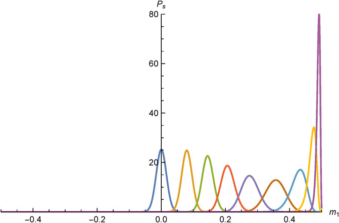
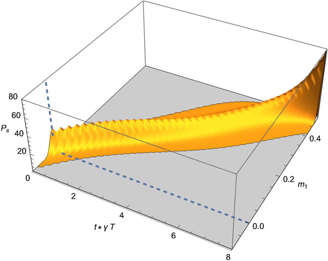
In Figure 1, the distribution of the magnetization is depicted at various times. In Figure 2, this evolution is represented in a plot.
3.6 -theorem and relaxation to equilibrium
The dynamical entropy of the distribution is defined as
As in Opus, we introduce a dynamical free energy:
which adds the term to the average of the free energy functional . With , Equation 5.36 yields.
For general functions and , partial summation yields
provided that the boundary terms at vanish. As discussed, this holds for but also for the logarithm in Equation 4.13 because we may insert a factor that makes this explicit. For , we now use the last expression, and for , we use the second one, which yields, also using Equation 4.10 and the property satisfied in (Equations 2.26, 2.27), the result
The various –factors are such that a term can be factored out to yield
With , and , this can finally be expressed as
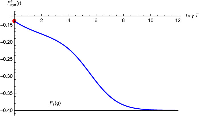
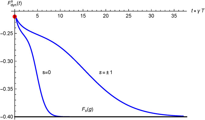
The last factors have the form , which is nonnegative, so that is a decreasing function of time. Dynamic equilibrium occurs when these factors vanish, which happens when the magnet has reached the thermodynamic equilibrium set by the Gibbs state and , with , as usual. The dynamical free energy (Equation 4.12) indeed ends up at the thermodynamic one,
This constitutes an example of the apparatus going dynamically to its lowest thermodynamic state and the pointer state indicating the measurement outcome . The temporal evolution from to is depicted in Figure 3.
3.7 Decoupling the apparatus
Near the end of the measurement, at a suitable time , the apparatus is decoupled from the system, by setting ; in doing so, an energy must be supplied to the magnet, which will then relax further its nearby minimum of the situation, to provide a stable pointer indication with a macroscopic order parameter that can be read off.
4 Dynamics of the spin-1 model
We now focus on the spin-1 case, in which the tested system, S, is , a spin-1 operator with having eigenvalues . Our magnet M has quantum spins-1 . According to Equation 2.5, one now deals with two order parameters,
While is the usual magnetization in the -direction, is a spin-anisotropy order parameter that discriminates the sectors with eigenvalues from the sector with eigenvalues .
The quantity , the operator-form of Equation 2.2, is our starting point for a permutation-invariant Hamiltonian that ensures unbiased measurement. Expanding the cosine, employing Equation 2.8 for each spin , and summing over yields a polynomial in the moments ,
For the Hamiltonian, we take as in Equation 3.2
It can be understood as containing the single-spin term , the pair couplings and , the triplet couplings and the quartet couplings , , and . However, note its different conception in Section 2.5.
At the initial time of the measurement, its state is described by its density matrix with elements for .
In each sector, M lies in its state , which is an operator that can be represented by a matrix. This exponential problem gets transformed into a polynomial one, a step that is exact for the considered mean-field-type Hamiltonian.
At , M is assumed to lie in a paramagnetic state, wherein the spins are fully disordered and uncorrelated. For each spin, its state is thus where . Multiplying by the respective element of leads to the elements of the initial density matrix of S + M in the sector,
For general angular momentum, the commutation relations and carry over to general spin
While we considered in Section 3, we now focus on .
We proceed as for spin . The commutator in Equation 2.29 does again not contribute. We introduce for . From Equation 5.5, it follows for general that
In the present case , this has nontrivial values
with Equation 5.6 implying that the term indeed drops out. The SO(3) generators
allow verifying these relations. Each of the has such a presentation. In Equation 2.30, the interchange of the with the will be needed. For , they commute, while for ,
Valid for , induction yields this for higher . For functions of the , , that can be expanded in a power series, it follows that
Now the can be eliminated using Equation 5.6, which leaves functions of only the , with the shifts in their arguments arising as the cost for this. As before, we can assume that , where is a scalar function of the eigenvalues of the . Valid at , this holds for , so it remains valid in time. Hence, it is possible to go from the matrix equations to scalar equations. With the equality in Equation 5.6 applied for spin , we end up with the scalar expressions
where for any function expandable in powers of the , it holds that
Now that all terms are scalar functions of the , it is seen that . We no longer need to track the operator structure and can work with scalar functions of the eigenvalues.
4.1 Off-diagonal sector: truncation of Schrödinger cat terms
In the spin Curie–Weiss model, it was found that the Schrödinger cat terms disappear by two mechanisms: dephasing of the magnet, possibly followed by decoherence due to the thermal bath. Similar behavior is now investigated for spin-1.
4.1.1 Initial regime: dephasing
Truncation of the density matrix (disappearance of the cat states) is a collective effect that takes place within an initial time window, in which the magnet stays in the paramagnetic phase, so that the mutual spin couplings and the coupling to the bath can be neglected. The spins of M act individually by their coupling to the tested spin S and do not get correlated yet. In the sector where the eigenvalue of the operator is , the Hamiltonian of the magnet is
At a given , this is a trace-free diagonal matrix with elements (twice) and ,
for . In this approximation, the density matrix of the magnet in each sector maintains the product structure (Equation 5.4) of uncorrelated spins at ,
where, setting , for each ,
Diagonal elements thus essentially do not evolve in this short-time window. The off-diagonal ones imply for
For small , this decays as with the dephasing time , very short for large . The undesired recurrences at , where the cosine equals 1 again, can be suppressed by assuming that the values in Equation 5.16 have a small spread (see Opus, Section 6.1.1). If the thermal oscillator bath has proper parameters, it will cause decoherence, as seen next.
4.1.2 Second step: decoherence
To include the bath in Equation 5.16, we now make the generalized Ansatz:
In the commutators (Equation 5.11), now reduces to the of Equation 5.14, and the terms are identical for all . We can neglect in the exponents of Equation 2.29 and find, putting in the minus terms,
with
Here, because the kernel is real valued; see the example in Equation 2.27, and
with a similar expression for , and finally
For , one has . For , one gets, using ,
because , , and . Therefore, for , this confirms that hardly any dynamics take place in this time window. In the next subsection, we show that they occur on a longer time scale .
For off-diagonal elements , it is seen that has terms and , so that
The exponentials are equal to unity, making , at the times , , encountered below Equation 5.17, when appearing in the dephasing process, and thus also as times where . To suppress recurrences like in the dephasing, we again set in each -term with small Gaussian distributed . For times well exceeding the coherence time of the bath, the and reach their finite limits, so that we have
The first part is small, and the second is given in Equation 5.24. After canceling out its exponents by the , an imaginary part remains. Hence, for , the terms can be neglected in . We keep
which is positive, so that with leads for large enough values of to a decoherence of the off-diagonal elements of the density matrix at the characteristic decoherence time and .
Decoherence is a combined effect of the apparatus spins; despite it, the individual elements of hardly decay in this time window, behaving as .
4.2 Registration dynamics for spin-1
In Section 3, a difference equation was derived for the distribution of the magnetization of the magnet for any number of spins-. Our aim here is to derive an analogous equation for the spin-1 case.
In the paramagnet, one has the form . Let with be the probability for a state of the magnet M characterized by the moments . It gathers the value for all sequences compatible with , the number of which is the degeneracy factor ,
with the and from Equation 2.14. The normalizations are
Due to the relations described by Equations 2.13 and 2.14 between the spin moments and the spin fractions , the shifts in induce the shifts and , with
which are integers, as they should be. The degeneracies for lead to the respective factors
where is used. The complicated last term is fortunately not needed, while the denominators of the first two will factor out.
Going to the functions of the moments , we proceed as for the spin situation. The terms of Equation 5.11 can again be combined and performing the -integrals in Equation 4.2 leads for to the kernel at the frequencies
for . Multiplying Equation 4.2 by and summing over , there results an evolution equation for the distribution at each discrete value of ,
Let us condense notation and introduce the shift operators and by their action
on any . They have the properties
Hence, Equation 5.32 can be expressed as
which has a remarkable analogy to Equation 4.9 and Equation 4.16 of Opus for the spin- case. By denoting above and , this is condensed further,
4.3 -theorem and relaxation to equilibrium
We now exhibit a theorem that assures the relaxation of the magnet towards its Gibbs equilibrium state and, thus, a successful measurement. The dynamical entropy of the distribution is defined as
Following Opus and Equation 4.12 above, we consider the dynamical free energy
It appears to depend on . The simultaneous change , implies that at all , as happened for in the spin case, but the differ from , except in the thermal situations at and .
With , not to be confused with the index , Equation 5.36 yields
For general functions with vanishing boundary terms, partial summation yields
For , we use the last expression, and for , we use the second one, while taking , and also using Equation 5.34 and the property satisfied generally in Equation 2.26, which yields the result
The various parts are such that a term can be factored out, to express this as
With , , and , this is equal to
The last factors have the form , which is nonnegative, implying that is a decreasing function of time. Dynamic equilibrium occurs when these factors vanish, which happens when the magnet has reached thermodynamic equilibrium, that is, the Gibbs state and , with , as usual. The dynamical free energy (Equation 5.38) then ends up at the thermodynamic free energy,
which actually does not depend on due to the invariance map of the static state, reflecting that the measurement is unbiased. This constitutes an explicit example of the apparatus going dynamically to its lowest thermodynamic state, the pointer state registering the measurement outcome.
Although the statics are identical for , this does not hold for the dynamics. While it is similar for (to change the sign of , also change the sign of ), this deviates from the dynamics. For , all are finite, but for , there are cases where vanishes, which leads to a slower dynamics; see Figure 5.
4.4 Numerical analysis
The initial spin-1 Hamiltonian leads to a matrix problem, which is numerically hard. For the considered mean-field-type model, the formulation in terms of the order parameters is exact; it lowers the dimensionality considerably. The variable can take values between 0 and 1. The value of indicates that of the take the value 0, while the other of the are . Given this number, can take values between and . Accounting for conservation of total probability, this leads to dynamical variables, a polynomial problem.
(Concerning higher spin: For spin , one separates terms with from those with ; for spin-2, one selects terms with , , or , etc.)
Equation 5.32 can be solved numerically as a set of linear differential equations. Programming it is straightforward; the vanishing of boundary terms and conservation of the total probability must be verified as a check on the code.
The magnet starts in the paramagnetic initial state
The sum of over equals unity and, with the mesh , so does its integral.
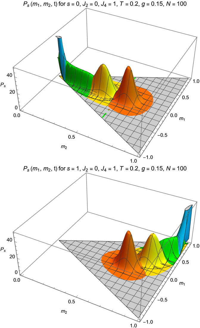
The dynamics (Equation 5.32) can be solved numerically, and the results are presented in upcoming figures. We consider the parameters, with large enough,
We plot in Figures 4A,B snapshots of at four times, for and . The case follows from the case by setting .
Figure 5 shows the evolution of the dynamical free energy .
4.5 Decoupling of the apparatus
Near the end of the measurement, the interaction between the system and the apparatus is cut off by setting ; in doing so, at decoupling time , Equation 5.13 expresses that an amount of energy
must be supplied to the magnet, leaving it with the post-decoupling free energy
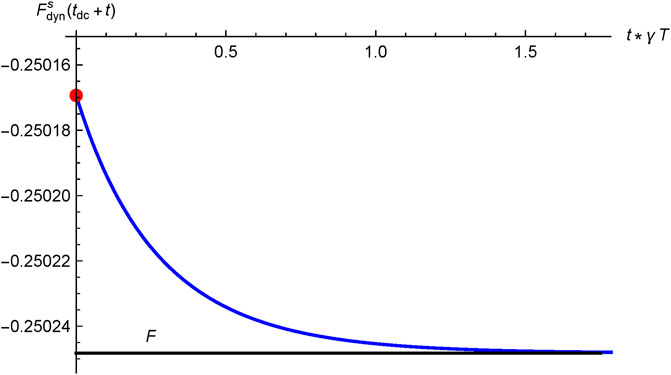
This post-decoupling state is not an equilibrium state; the magnet will now relax to the nearby minimum of the case. There follows a relaxation driven by bath, with the magnet evolving under the Hamiltonian to its Gibbs state , with free energy .
When the decoupling time is large enough, the magnet M lies in its Gibbs state at coupling , . Due to the invariance of the situation, the approach to it is identical for starting in any of the sectors .
To compare with the dynamics that end up in one of the minima, one must restrict the Gibbs state, which has three degenerate minima, to the nearby minimum. This is achieved numerically even at moderate by discarding well away from the peak of , also in . For , it suffices to keep for ; for by doing that for .
The change of the state is also seen in . Let us consider the sector , where at all . Here, the coupling has the tendency to suppress , so after decoupling, will relax to a larger value. For , we get from the Gibbs states at and at , respectively,
The full-time behavior for and couplings as in Equation 5.46 is presented in Figure 6, with the finite- values increasing from to .
The relaxation in the sectors follows immediately from this. The map (Equation 5.50) yields. The maps (4.11) and (4.13) of Models lead to
4.6 Energy cost of quantum measurement
The Copenhagen postulates obscure one of the facts of life in a laboratory: a firm cost for the energy needed to keep the setup running. In this work, we consider two intrinsic costs. In the previous subsection, we established the cost of decoupling the apparatus from the system. Here, we consider resetting the magnet for another run. It must be set from its stable state back to its metastable state. Being related to the magnet, both costs are macroscopic.
Our initial state, the paramagnet (pm), has zero magnetic energy and maximal entropy
The energy needed to reset the Gibbs state of the magnet to the paramagnetic one is
It is evidently macroscopic. The condition that is positive was identified in Opus and in Models as the condition that the initial paramagnetic state is metastable but not stable.
5 Conclusion
This article dealt with the dynamics of an ideal quantum measurement of the -component of a spin-1. The statics for this task were worked out recently in our “Models” article (Nieuwenhuizen, 2022); it generalized to any spin the Curie–Weiss model to measure a spin ; the latter was considered in great detail in “Opus” (Allahverdyan et al., 2013). Here, we first reformulated the dynamics of the known case for spin and worked out some further properties. The resulting formalism is suitable as a basis for models to measure any higher spin.
The dynamics of measurement in the spin-1 case were analyzed in detail. Off-diagonal elements of the density matrix (“cat states”) were shown to decay very fast (“truncation of the density matrix”) due to dephasing, possibly followed by decoherence.
The evolution of the diagonal elements of the density matrix was expressed as coupled first-order differential equations for the distribution of two magnetization-type-order parameters, . The approach to a Gibbs equilibrium was certified by demonstrating a -theorem. The resulting scheme was found to be numerically a polynomial problem. These are easily solved with the present power of laptops for an apparatus consisting of a few hundred spins. The evolution of the probability density was evaluated, and the -theorem was verified. The macroscopic energy costs for decoupling the apparatus from the spin and for resetting it from its stable state to its metastable state for use in the next run of the measurement were quantified.
For general spin , this method simplified the numerically hard problem of dimension by a polynomial problem of order for its -order parameters. For more complicated models of the apparatus, it will likewise pay off to focus on the order parameter of the dynamical phase transition of the pointer that achieves the registration of the measurement. The fact that the phase transition in the magnet is of first order underlines that our mean-field-type models, although of mathematical convenience, are not essential for the fundamental description of quantum measurements.
Data availability statement
The original contributions presented in the study are included in the article/supplementary material; further inquiries can be directed to the corresponding author.
Author contributions
TN: writing – original draft and writing – review and editing.
Funding
The author(s) declare that no financial support was received for the research and/or publication of this article.
Conflict of interest
The author declares that the research was conducted in the absence of any commercial or financial relationships that could be construed as a potential conflict of interest.
Generative AI statement
The author(s) declare that no Generative AI was used in the creation of this manuscript.
Publisher’s note
All claims expressed in this article are solely those of the authors and do not necessarily represent those of their affiliated organizations, or those of the publisher, the editors and the reviewers. Any product that may be evaluated in this article, or claim that may be made by its manufacturer, is not guaranteed or endorsed by the publisher.
Footnotes
1An analogy is offered by the dark matter problem in cosmology. Abandoning particle dark matter, we view dark “matter” as a form of energy and assume new properties of vacuum energy. This provides a description of black holes with a core rather than a singularity (Nieuwenhuizen, 2023), aspects of dark matter throughout the history and future of the Universe (Nieuwenhuizen, 2024a), and the giant dark matter clouds around isolated galaxies (Nieuwenhuizen, 2024b), explaining the “indefinite flattening” of their rotation curves (Mistele et al., 2024). Remarkably, this approach is a generalization of the classical Lorentz–Poincaré electron—a charged, non-spinning spherical shell filled with vacuum energy (Nieuwenhuizen, 2025).
2To simplify the notation, we replace the standard notation for spins with and . For an angular momentum , the model also applies to the measurement of with eigenvalues . We employ units .
3For the connection with the parameters in Opus, see ref 1.
References
Allahverdyan, A. E., Balian, R., and Nieuwenhuizen, T. M. (2003b). Curie-Weiss model of the quantum measurement process. EPL Europhys. Lett. 61, 452–458. doi:10.1209/epl/i2003-00150-y
CrossRef Full Text | Google Scholar
Allahverdyan, A. E., Balian, R., and Nieuwenhuizen, T. M. (2005a). The quantum measurement process in an exactly solvable model. AIP Conf. Proc. 750, 26–34. doi:10.1063/1.1874554
CrossRef Full Text | Google Scholar
Allahverdyan, A. E., Balian, R., and Nieuwenhuizen, T. M. (2005b). Dynamics of a quantum measurement. Phys. E Low-dimensional Syst. Nanostructures 29, 261–271. doi:10.1016/j.physe.2005.05.023
CrossRef Full Text | Google Scholar
Allahverdyan, A. E., Balian, R., and Nieuwenhuizen, T. M. (2006). Phase transitions and quantum measurements. AIP Conf. Proc. 810, 47–58. doi:10.1063/1.2158710
CrossRef Full Text | Google Scholar
Allahverdyan, A. E., Balian, R., and Nieuwenhuizen, T. M. (2007). “The quantum measurement process: lessons from an exactly solvable model,” in Beyond the quantum (World Scientific), 53–65.
Google Scholar
Allahverdyan, A. E., Balian, R., and Nieuwenhuizen, T. M. (2013). Understanding quantum measurement from the solution of dynamical models. Phys. Rep. 525, 1–166. doi:10.1016/j.physrep.2012.11.001
CrossRef Full Text | Google Scholar
Allahverdyan, A. E., Balian, R., and Nieuwenhuizen, T. M. (2017). A sub-ensemble theory of ideal quantum measurement processes. Ann. Phys. 376, 324–352. doi:10.1016/j.aop.2016.11.001
CrossRef Full Text | Google Scholar
Allahverdyan, A. E., Balian, R., and Nieuwenhuizen, T. M. (2024). Teaching ideal quantum measurement, from dynamics to interpretation. Comptes Rendus. Phys. 25, 251–287. doi:10.5802/crphys.180
CrossRef Full Text | Google Scholar
Allahverdyan, A. E., Balian, R., and Nieuwenhuizen, T. M. (2025). Interpretation of quantum mechanics from the dynamics of ideal measurement. Europhys. News, appear 56, 23–25. doi:10.1051/epn/2025210
CrossRef Full Text | Google Scholar
Auffèves, A., and Grangier, P. (2016). Contexts, systems and modalities: a new ontology for quantum mechanics. Found. Phys. 46, 121–137. doi:10.1007/s10701-015-9952-z
CrossRef Full Text | Google Scholar
Auffèves, A., and Grangier, P. (2020). Deriving born’s rule from an inference to the best explanation. Found. Phys. 50, 1781–1793. doi:10.1007/s10701-020-00326-8
CrossRef Full Text | Google Scholar
Ballentine, L. E. (1970). The statistical interpretation of quantum mechanics. Rev. Mod. Phys. 42, 358–381. doi:10.1103/revmodphys.42.358
CrossRef Full Text | Google Scholar
De Broglie, L. (1924). Recherches sur la théorie des quanta. Paris: Migration-université en cours d’affectation. PhD thesis.
Google Scholar
Donker, H., De Raedt, H., and Katsnelson, M. (2018). Quantum dynamics of a small symmetry breaking measurement device. Ann. Phys. 396, 137–146. doi:10.1016/j.aop.2018.07.010
CrossRef Full Text | Google Scholar
Mistele, T., McGaugh, S., Lelli, F., Schombert, J., and Li, P. (2024). Indefinitely flat circular velocities and the baryonic tully–Fisher relation from weak lensing. Astrophysical J. Lett. 969, L3. doi:10.3847/2041-8213/ad54b0
CrossRef Full Text | Google Scholar
Nieuwenhuizen, T. M. (2023). Exact solutions for black holes with a smooth quantum core. arXiv Prepr. arXiv:2302.14653.
Google Scholar
Nieuwenhuizen, T. M. (2024a). Solution of the dark matter riddle within standard model physics: from black holes, galaxies and clusters to cosmology. Front. Astronomy Space Sci. 11, 1413816. doi:10.3389/fspas.2024.1413816
CrossRef Full Text | Google Scholar
Nieuwenhuizen, T. M. (2024b). Indefinitely flat rotation curves from Mpc sized charged cocoons. Europhys. Lett. 148, 49002. doi:10.1209/0295-5075/ad895f
CrossRef Full Text | Google Scholar
Nieuwenhuizen, T. M. (2025). How the vacuum rescues the Lorentz electron and imposes its Newton and geodesic motion, and the equivalence principle, to appear Eur. J. Phys.
Google Scholar
Nieuwenhuizen, T. M., Perarnau-Llobet, M., and Balian, R. (2014). Lectures on dynamical models for quantum measurements. Int. J. Mod. Phys. B 28, 1430014. doi:10.1142/s021797921430014x
CrossRef Full Text | Google Scholar
Perarnau-Llobet, M., and Nieuwenhuizen, T. M. (2017a). Simultaneous measurement of two noncommuting quantum variables: solution of a dynamical model, Physical Review A 95 (5), 052129.
CrossRef Full Text | Google Scholar
Perarnau-Llobet, M., and Nieuwenhuizen, T. M. (2017b). Dynamics of quantum measurements employing two Curie--Weiss apparatuses, Philosophical Transactions of the Royal Society A: Mathematical, Physical and Engineering Sciences, 375 (2106), 20160386.
PubMed Abstract | CrossRef Full Text | Google Scholar
Schrödinger, E. (1926). An undulatory theory of the mechanics of atoms and molecules. Phys. Rev. 28, 1049–1070. doi:10.1103/physrev.28.1049
CrossRef Full Text | Google Scholar
Van Den Bossche, M., and Grangier, P. (2023). Contextual unification of classical and quantum physics. Found. Phys. 53, 45. doi:10.1007/s10701-023-00678-x
CrossRef Full Text | Google Scholar
Wheeler, J. A., and Zurek, W. H. (2014). Quantum theory and measurement, 15. Princeton University Press.
Google Scholar
 Theodorus Maria Nieuwenhuizen