Short-term soil moisture content forecasting with a hybrid informer model

This study proposes a novel time-series forecasting approach that integrates the Informer model with the RAO − 1 optimization algorithm for soil water content (SWC) prediction. The method innovatively combines Informer’s long-range dependency modeling with RAO-1’s efficient hyperparameter optimization to enhance forecasting accuracy. Comparative experiments were conducted using Random Forest, Support Vector Regression, Long Short-Term Memory and Transformer as baseline models on SWC datasets from the Beijing region. The RAO-1-optimized Informer consistently outperforms these baselines in both deterministic and probabilistic forecasting tasks, while also achieving superior computational efficiency. These results highlight the robustness of the proposed method and its potential to support sustainable agricultural water management through accurate SWC prediction.

1 Introduction

Soil water content (SWC) as a critical parameter in the hydrological cycle, plays a pivotal regulatory role in regional water resource sustainability and agricultural productivity (Chen et al., 2025; Liu et al., 2020). Accurate prediction of SWC dynamics enables optimized irrigation scheduling, water waste reduction, and crop water use efficiency (WUE) improvement. Research demonstrates that in arid regions, precision irrigation strategies based on SWC monitoring can reduce water resource consumption by 15–30% while maintaining or even increasing crop yields (Gundim et al., 2023). Under global climate change scenarios characterized by uneven spatiotemporal precipitation distribution, the increasing frequency of extreme drought and flood events highlights the importance of SWC monitoring. SWC data not only facilitates drought risk prediction and planting strategy optimization to ensure food security (Bonfante et al., 2019), but also enables early flood warnings through real-time SWC analysis. When SWC approaches saturation capacity, integrating meteorological data allows prediction of surface runoff and waterlogging probability, thereby supporting drainage measures to mitigate flood impacts (Azimi et al., 2020). Thus, SWC prediction holds significant application value across multiple domains, including water resource management, sustainable agricultural development, and disaster prevention.

Prediction methods for SWC can generally be categorized into three main types: traditional physical models, machine learning (ML) techniques, and deep learning (DL) approaches (Mahesh, 2020). As noted by Karandish and Šimůnek (2016), numerical models and machine learning models each have their strengths in soil moisture simulation, with data-driven methods offering flexibility in handling complex nonlinear relationships. Physically-based models use meteorological data as boundary conditions to simulate target processes (e.g., soil water dynamics), thus their accuracy depends on the quality and completeness of these meteorological inputs. While they do not model atmospheric processes in detail, they do rely on a descriptive representation of meteorological conditions as inputs. However, physical models generally require numerous input parameters, including high-resolution soil, vegetation, and meteorological data, which are difficult to collect comprehensively for large-scale or regional applications. This critical limitation has been noted in recent reviews (Singh et al., 2023; Mohanty et al., 2017). According to Singh et al. (2023), the lack of detailed input parameters substantially restricts the effectiveness of physical approaches in SWC measurement. Mohanty et al. (2017) further emphasize that the spatial–temporal heterogeneity and data gaps in environmental variables pose significant obstacles for effective large-scale SWC modeling using physical approaches.

While physically-based models such as the Integrated Farm System Model (IFSM) (Jégo et al., 2015) and Soil and Water Assessment Tool (SWAT) (Verma et al., 2022) offer mechanistic insights into soil water dynamics and are widely validated in hydrological research, their time consumption is generally much lower than that of any ML model, especially in terms of per-run or operational use. For instance, models like IFSM are specifically designed for efficient scenario analysis and farm-level decision support, featuring extremely low computational demands compared to all data-driven ML approaches (Antle et al., 2017). However, the computational burden of physical models can increase with expanding spatial scales, complex heterogeneity, or high temporal resolutions, due to the need for intensive numerical calculations in process-based simulations (Tekle et al., 2025). Furthermore, the overall complexity and numerical procedures underlying these models can sometimes restrict their application to extremely rapid, large-scale or real-time tasks.

The computational efficiency of both physical and machine learning models is, in fact, highly context-dependent. Depending on the specific implementation, model configuration, and the scale of the target problem, different approaches may exhibit varying levels of computational demand. For example Jégo et al. (2015) reported that IFSM achieved rapid simulation times in farm-scale applications, whereas Tekle et al. (2025) found that physical models could become computationally intensive for large basin-scale or long-term simulations. Similarly, as reviewed by Benos et al. (2021), machine learning methods such as artificial neural networks (ANNs) and Convolutional Neural Networks (CNNs) have achieved promising results for SWC prediction across various agricultural applications. However, the computational complexity of these models tends to increase substantially when dealing with high-dimensional data or more frequent retraining, especially for deep neural network architectures. Therefore, care should be taken to evaluate computational trade-offs in light of the specific modeling context, rather than making generalized assumptions about one model class always outperforming another.

To overcome some of these constraints, data-driven approaches—particularly those employing ML and DL algorithms—have attracted increasing attention for SWC prediction in recent years (Reichstein et al., 2019). These approaches are valued for their flexibility and ability to capture nonlinear relationships, and can be robust even with incomplete or noisy input data (Ali et al., 2015). However, it is important to note that not all ML techniques are computationally efficient: while some simple models, such as decision trees or small support vector machines, can provide rapid inference with moderate training requirements (Seydi et al., 2023), many ML and especially DL methods, such as deep neural networks, can be far more time-consuming than IFSM-type physical models, particularly during training or when processing large-scale datasets and frequent retraining is required (Reichstein et al., 2019). Therefore, despite their advantages in some predictive contexts, ML and DL models may not always offer faster operational performance than well-optimized process-based physical models.

Therefore, despite their advantages in some predictive contexts, ML and DL models may not always offer faster operational performance than well-optimized process-based physical models.

Nevertheless, recent comparative studies have shown that certain ensemble ML algorithms can achieve both high accuracy and satisfactory computational efficiency, particularly in small-sample settings.

Teshome et al. (2024) conducted a comprehensive evaluation of several widely used ML algorithms, including XGBoost (Niazkar et al., 2024), LightGBM (Niazkar et al., 2024), CatBoost (Hancock and Khoshgoftaar, 2020), Random Forest (Sun et al., 2024), and k-Nearest Neighbors (Halder et al., 2024). Their study showed that ensemble learning models—particularly XGBoost and LightGBM—consistently achieved high accuracy and computational efficiency, especially in small-sample settings. Despite these strengths, traditional ML approaches exhibit key limitations, such as constrained generalization across heterogeneous landscapes, limited feature interpretability, and a reliance on manual feature engineering. Moreover, their capacity to capture the complex spatiotemporal dependencies inherent in environmental systems remains limited (Reichstein et al., 2019; Xu and Liang, 2021).

To overcome these challenges, researchers have turned to DL techniques, which are characterized by multilayer neural architectures capable of learning complex nonlinear relationships from high-dimensional data. For instance, Azmat et al. (2022) proposed a Temporal Graph Convolutional Network (T-GCN) that incorporates domain knowledge and constructs graph structures via clustering to model both spatial and temporal dependencies in SWC dynamics. Similarly, Batchu et al. (2022) developed a convolutional regression model that integrates multi-source remote sensing data—such as Sentinel-1, Sentinel-2, and Soil Moisture Active Passive (SMAP)—leading to enhanced spatial resolution and predictive accuracy. However, DL models also present several challenges, including high computational costs, complex architectures, and the need for extensive data preprocessing. These factors limit their scalability and practical deployment in real-time or resource-constrained environments. Furthermore, the generalizability of DL models across different soil types and geographic conditions remains insufficiently validated.

In response to the limitations of both traditional ML and advanced DL methods, hybrid approaches have been proposed. For example, Liu et al. (2024) introduced a model that combines a backpropagation (BP) neural network with genetic algorithm-based feature selection. This approach leverages Sentinel remote sensing data to reduce redundant input features, thereby improving computational efficiency while maintaining high predictive accuracy. Nonetheless, the model’s performance remains sensitive to the quality and temporal consistency of remote sensing inputs, which can impact its robustness in operational settings. In summary, although ML and DL techniques offer promising avenues for accurate SWC prediction, significant challenges remain—particularly in terms of data quality sensitivity, computational demands, and model generalizability. Addressing these limitations is essential to enable reliable, large-scale, and real-time applications in diverse agricultural and environmental contexts.

To address the aforementioned challenges, this study proposes an improved Informer model optimized by the RAO-1 algorithm for multi-step prediction of SWC. The model is capable of effectively predicting the variation trends of SWC at depths of 10 cm, 20 cm, and 30 cm below the surface for the next 1, 2, and 3 days, thereby providing valuable scientific support for agricultural management and ecological monitoring. Specifically, the model leverages historical observational data — including temperature, precipitation, evaporation, and soil water content — as input features to enhance the model’s capability for time series forecasting and improve prediction accuracy for SWC.

In terms of model architecture, building upon the core advantages of the Informer framework, the model employs the ProbSparse self-attention mechanism, which reduces the computational complexity of self-attention from $O\left(L^2\right)$in the original Transformer architecture to $O\left(L\mathit{\text{logL}}\right)$ (Zhu et al., 2023). This significantly improves computational efficiency, particularly when handling long-sequence data. Furthermore, by incorporating the concept of local sensitivity, the model is better able to capture local dependencies among input variables, enabling it to more effectively learn the dynamic patterns underlying SWC variations. To further enhance the model’s performance, the RAO-1 algorithm is integrated for adaptive hyperparameter optimization. As a parameter-free global optimization algorithm, RAO-1 dynamically adjusts the search step size, effectively mitigating the risk of premature convergence commonly encountered in traditional optimization methods (Rao, 2020). Through the application of RAO-1, the model achieves superior convergence behavior during hyperparameter search, substantially improves computational efficiency, and reduces training time, thus offering a practical and scalable solution for large-scale SWC prediction tasks.

To validate the effectiveness of the proposed RAO-1 optimized Informer model for soil moisture prediction, we conducted comparative experiments with three state-of-the-art (SOTA) baseline models: Random Forest (RF), Long Short-Term Memory (LSTM), and Transformer. These models were selected as they represent both traditional ML approaches and advanced DL architectures that are widely recognized in time-series and remote sensing analysis.

The performance of all models was quantitatively evaluated using five commonly adopted regression metrics: Mean Squared Error (MSE) (Wang and Lu, 2018), Root Mean Squared Error (RMSE) (Wang and Lu, 2018), Mean Absolute Error (MAE) (Wang and Lu, 2018), Mean Absolute Percentage Error (MAPE) (Ren and Glasure, 2009), and the coefficient of determination (R²) (Berggren, 2024). These metrics offer comprehensive insights into both the absolute and relative prediction errors, as well as the explanatory power of the models.

Experimental results demonstrate that the RAO-1 optimized Informer consistently outperforms all baseline models across multiple evaluation metrics. Specifically, our model achieves the lowest MSE, RMSE, MAE, and MAPE values, and the highest R² score, indicating superior predictive accuracy and generalization ability for soil moisture content estimation. These findings confirm the effectiveness of integrating Rao-1 based hyperparameter optimization with the Informer architecture, and highlight its advantage over both conventional and state-of-the-art methods in this domain.

The main contribution of this paper can be summarized as:

1. We trained the Informer model using only a limited set of input features while still achieving satisfactory performance.

2. We employed the RAO-1 algorithm for hyperparameter optimization, which not only improved the convergence performance during the hyperparameter search process but also significantly enhanced the overall computational efficiency and reduced the training time.

3. We conducted a comparative analysis with the widely used baseline models in the field of time series forecasting to validate the effectiveness of the proposed approach.

The remainder of this paper is structured as follows. Section 2 introduces the predictive model. Section 3 provides the experimental results and corresponding analysis. Conclusions are drawn in Section 4.

2 The proposed method

To improve the forecasting performance of the Informer model, we employ the RAO-1 algorithm for adaptive hyperparameter optimization. The proposed method is illustrated in Figure 1.

Figure 1

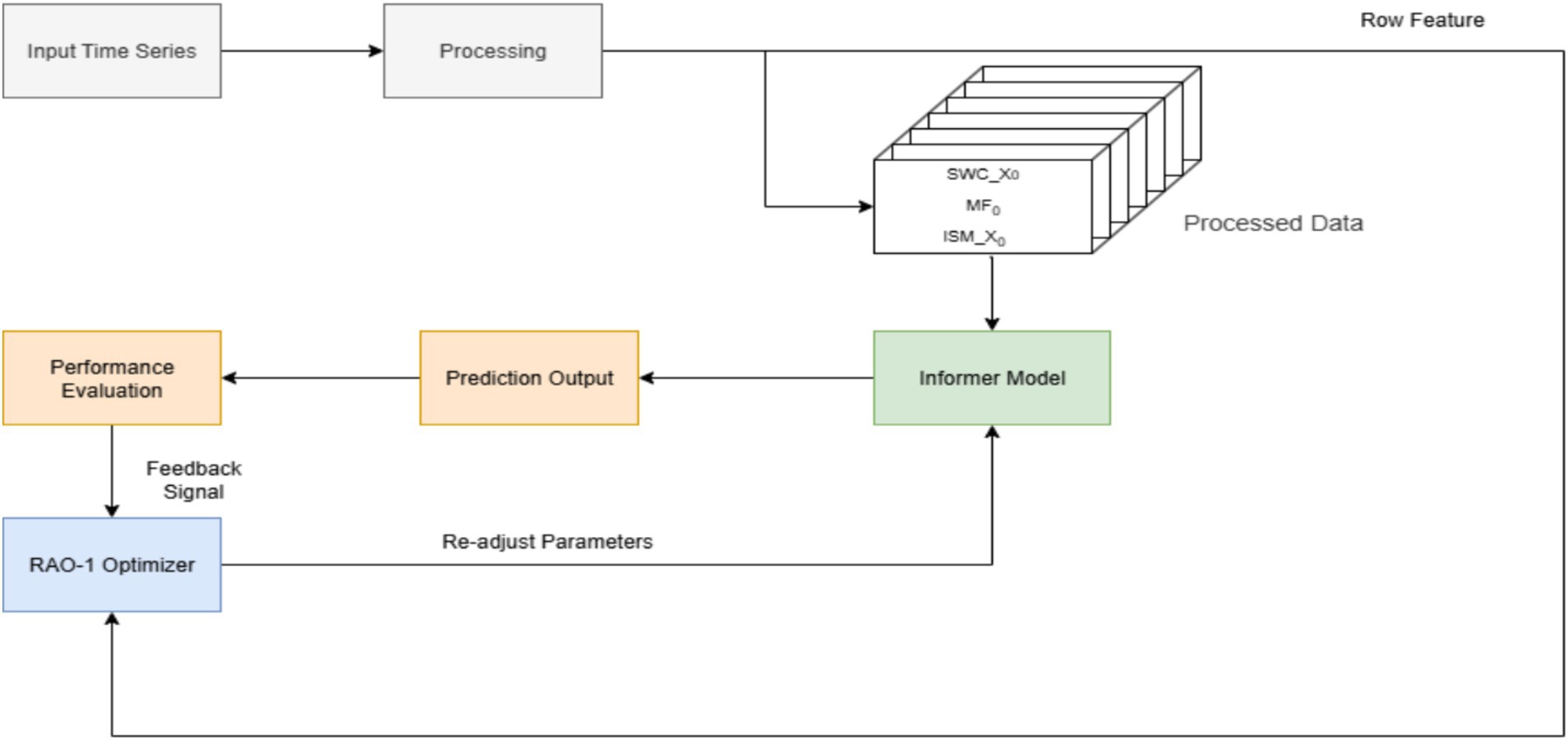
Figure 1. Method diagram of using RAO-1 to optimize the informer model.

As shown in Figure 1, the method consists of four main stages: raw time series data is first preprocessed to handle missing values, normalize features, and convert data formats to ensure compatibility with the Informer input format.

In the preprocessing stage, for each time step, we align the time stamps of meteorological features (MF), soil water content at depth X (SWC_X), and the initial soil moisture at the same depth (ISM_X). These variables corresponding to the same date are concatenated to form a multivariate feature vector. This procedure is repeated for all time steps to generate the input matrix for the subsequent model, with each row representing the features for one specific timestamp.

The Informer model is initially trained using a set of hyperparameters. After training, the model’s forecasting performance is evaluated by a fitness function measuring prediction accuracy. If the fitness value does not meet predefined criteria, the RAO-1 algorithm adaptively generates new hyperparameters based on current performance feedback. The Informer model is then retrained with updated hyperparameters. This evaluation and optimization cycle repeats until convergence or stopping conditions are satisfied.

2.1 Data source and feature extraction

The dataset employed in this study was collected from a single in-situ monitoring site in Beijing, China (39.48°N, 116.28°E), providing point-based measurements rather than spatially averaged data. Observations were recorded once per day from February to November of each year between 2012 and 2016. Each daily entry comprised a suite of meteorological features—mean air temperature, atmospheric pressure, relative humidity, surface temperature, precipitation, evaporation, and sunshine duration—as well as SWC and initial soil moisture (ISM) at three depths (10 cm, 20 cm, and 30 cm). Guided by domain knowledge regarding the factors influencing soil moisture dynamics, daily mean air temperature, precipitation, evaporation, relative humidity, and the historical soil water content at each respective depth were selected as the fundamental input features for the predictive model. All variables were temporally aligned according to date and concatenated into multivariate input vectors.

2.2 Data pre-processing

Prior to model training, missing values in both soil moisture and meteorological records were addressed using linear interpolation to ensure data continuity. At each time step, the temporally aligned meteorological variables, the corresponding SWC at depth X, and ISM at the same depth (defined as SWC at the start of each day) were incorporated into unified feature vectors. To account for seasonal effects on soil moisture, the dataset was partitioned into the full season—comprising all observations from February to November each year—and the rainy season (June to August), which represents the period of peak precipitation in Beijing and forms a strict subset of the full seasonal dataset following regional climatological conventions. All input features were standardized using Z-score normalization to mitigate disparities in magnitude and facilitate model convergence. Supervised learning samples were constructed using a sliding window approach: observations from the preceding 7 days were used as input to predict SWC for the subsequent 3 days, enabling the Informer model to capture short- to medium-term temporal dependencies. Through this systematic pre-processing and feature engineering process, a high-quality and well-structured dataset was established, providing a robust foundation for model training and evaluation under varying meteorological and hydrological conditions.

2.3 Informer module

The Informer model, proposed by Zhou et al. (2020), is an efficient and scalable Transformer-based architecture specifically designed for long sequence time-series forecasting. Similar to the long sequence forecasting model applied in ship motion attitude prediction by Hou et al. (2024), Informer addresses the computational complexity issues of traditional Transformer architectures. Unlike the original Transformer, which suffers from quadratic time and space complexity with respect to sequence length, Informer introduces several innovative techniques to significantly reduce computational cost while maintaining high forecasting accuracy.

The Transformer-based models have demonstrated remarkable performance in sequence modeling tasks. However, their self-attention mechanisms suffer from high computational complexity, particularly when dealing with long sequences. To address this challenge, the Informer model incorporates a ProbSparse Self-Attention mechanism that selectively focuses on the most critical attention scores. This selective attention reduces the computational burden by identifying and retaining only the top- $u$ queries with the largest sparsity measurements, resulting in a significant reduction of time complexity from $O\left(L^2\right)$to $O(LlogL)$ , where $L$ represents the sequence length (Zhu et al., 2023). This approach accelerates attention computation and effectively handles long sequences. The architecture of the Informer model is illustrated in Figure 2.

Figure 2

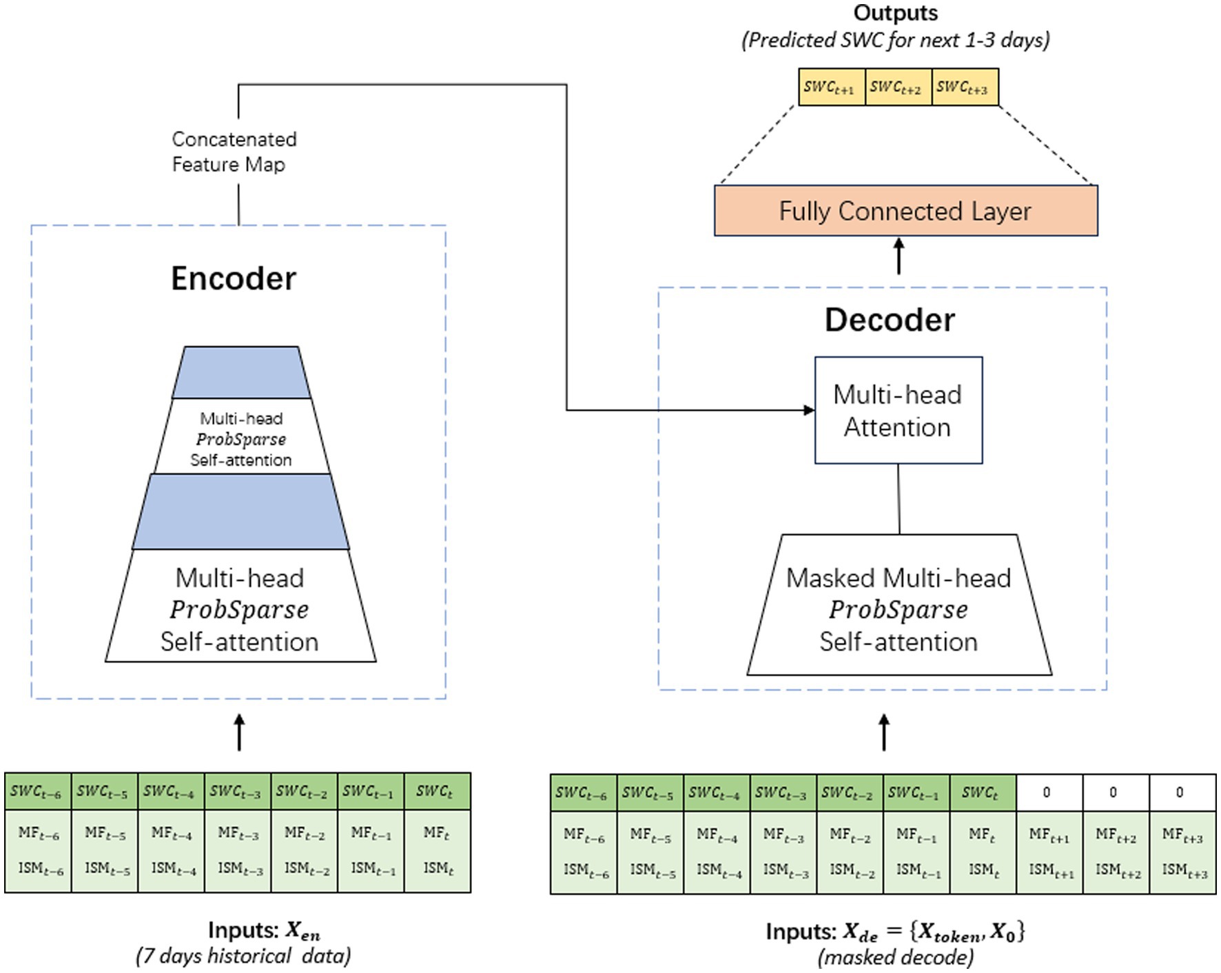
Figure 2. The architecture of the informer model.

The Informer model consists of the following key components:

Input Embedding: The Informer model begins with an input embedding layer that handles two input streams: the encoder input ( $X_{\mathit{en}}$ ) and the decoder input ( $X_{\mathit{de}}$ ). The encoder input consists of multivariate time series features over seven consecutive historical days, combining both SWC at the target depth and associated meteorological variables including daily average temperature, precipitation, humidity, etc. The decoder input includes these historical tokens followed by a series of zero-masked tokens corresponding to the forecast horizon (next 3 days). Each input sequence is projected into a higher-dimensional feature space through a linear transformation, as defined in Equation (1):

$\begin{array}{ll}{X}_e=W_{e}X+b_e& (1)\end{array}$

where $X$ is the input sequence, $W_e$ is the embedding matrix, and $b_e$ is the bias term.

Encoder-Decoder Architecture: Similar to the original Transformer, Informer utilizes an encoder-decoder architecture, but with optimizations in the attention mechanism. The encoder generates a representation of the input sequence, which is then passed to the decoder for prediction.

Self-attention mechanism: The self-attention mechanism, which calculates attention scores between all pairs of tokens in the input sequence, is a fundamental component of the Transformer and Informer architectures. However, this mechanism suffers from quadratic complexity in relation to the sequence length. To address this, Informer introduces the probSparse attention mechanism, which reduces the complexity by focusing on the most informative parts of the sequence. This reduces the complexity from $O\left(L^2\right)$to $O(LlogL)$ .

The self-attention mechanism can be mathematically formulated as shown in Equation (2):

$\begin{array}{ll}\mathit{\text{Attention}}(Q,K,V)=\mathit{\text{softmax}}\left(\frac{\overline{Q}{K}^T}{\sqrt{d_k}}\right)V& (2)\end{array}$

where $Q$ , $K$ , and $V$ are the query, key, and value matrices, respectively, and $d_k$ is the dimension of the key vectors.

ProbSparse attention: To further optimize the attention computation, Informer introduces an approximation called ProbSparse attention. This mechanism selectively focuses on the most informative queries, while ignoring irrelevant parts of the sequence. The sparsity score $u_q$ for each query is computed as shown in Equation (3):

$\begin{array}{ll}{u}_q=\sum _{k=1}^l{e}^{\left(\frac{q\cdot k}{\sqrt{d_k}}\right)}& (3)\end{array}$

where $q$ and $k$ are the query and key vectors, respectively, and $d_k$ is the dimension of the key vectors.

Only the queries with the top- $u$ values of $u_q$ are retained, ensuring that the most relevant query-key pairs dominate the attention distribution. This approach significantly reduces computational costs by focusing attention only on the most critical parts of the sequence.

Decoder: The decoder in the Informer architecture consists of stacked layers incorporating masked multi-head ProbSparse self-attention and standard multi-head attention. The decoder input sequence $X_{\mathit{de}}$comprises the concatenated historical multivariate features and masked tokens for the future forecasting steps. The masked ProbSparse self-attention enforces the causal constraint by limiting the decoder’s access to previous and current positions only, thereby eliminating any leakage of future information during training and inference. Furthermore, the decoder integrates the output from the encoder via standard multi-head attention, allowing it to leverage comprehensive contextual information from historical soil moisture and meteorological data. This design enables the decoder to generate rich hidden representations embedding essential temporal dependencies and feature correlations, which are used to produce accurate future soil moisture content forecasts.

Prediction layer: The output of the decoder is processed by a fully connected layer to produce the final multi-step forecast. Specifically, the last hidden state from the decoder, $h_{\mathit{\text{decoder}}}$ , is transformed as shown in Equation (4):

$\begin{array}{ll}\widehat{Y}=W_d{h}_{\mathit{\text{decoder}}}+b_d& (4)\end{array}$

where $W_d$ and $b_d$ are the corresponding weight matrix and bias for the output layer. This operation yields the predicted SWC values for the subsequent 1–3 days, as indicated at the output node of Figure 2. This final step translates the learned temporal features into concrete forecasts, thereby completing the end-to-end prediction process of the Informer model.

Informer presents a breakthrough in time-series forecasting by addressing the limitations of traditional attention mechanisms. Its design principles, including sparse attention and sequence distillation, enable efficient handling of long sequences while maintaining strong predictive performance. However, the parameter optimization process of the Informer model remains relatively complex, which can hinder its computational efficiency and prolong training time, especially when dealing with large-scale time series data. To address this challenge, we employ the RAO-1 optimization algorithm to fine-tune the parameters of the Informer model. By integrating RAO-1, a metaheuristic optimization technique known for its simplicity and effectiveness in navigating complex search spaces, we aim to enhance the convergence speed and overall computational efficiency of the training process. This integration not only accelerates model training but also contributes to achieving more stable and reliable forecasting performance.

2.4 The hybrid informer model

To further enhance the training efficiency and parameter optimization capability of the Informer model, we integrate the RAO-1 algorithm—a robust, parameter-free metaheuristic optimizer renowned for its simplicity and competitive performance in complex optimization tasks. The name ‘RAO-1’ stands for ‘Rao Algorithm 1,’ reflecting its introduction as the first simple, metaphor-less population-based metaheuristic optimization algorithm by Rao (Rao, 2020). The intuition behind RAO-1 is to guide the search process by encouraging all candidate solutions in the population to move closer to the best solution and further away from the worst, thereby promoting effective exploitation and exploration without the need for algorithm-specific control parameters or metaphorical inspirations.

ALGORITHM 1

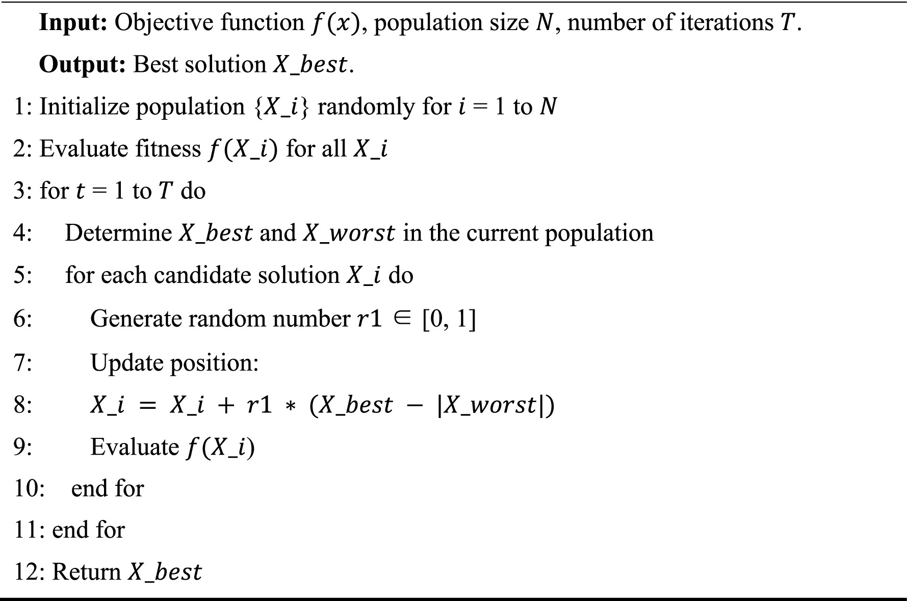
ALGORITHM 1. RAO-1 optimization algorithm.

Unlike traditional evolutionary algorithms that rely on control parameters, such as crossover and mutation operations, RAO-1 employs a direct approach to updating candidate solutions. The detailed implementation steps of this procedure are outlined in Algorithm 1, which presents the RAO-1 optimization algorithm. We strictly follow the update rule as defined in the original RAO-1 paper (Rao, 2020), as shown in Equation (5):

$\begin{array}{ll}{X}_i^{(t+1)}=X_i^{\left(t\right)}+r_1\cdot (X_{\mathit{\text{best}}}^{\left(t\right)}-\mid X_{\mathit{\text{worst}}}^{\left(t\right)}\mid )& (5)\end{array}$

where all notations are consistent with (Rao, 2020): $X_i^{\left(t\right)}$is the position of candidate $i$ at iteration $t$ , $X_{\mathit{\text{best}}}^{\left(t\right)}$ and $X_{\mathit{\text{worst}}}^{\left(t\right)}$ denote the best and worst solutions at iteration $t$ , $r_1$ is a randomly generated number within the range $[0,1]$ , $\mid \cdot \mid$ represents the element-wise absolute value operation.

The key design philosophy of RAO-1 is to encourage exploration toward optimality while maintaining population diversity, thus helping to prevent premature convergence—a property that is particularly beneficial for navigating the high-dimensional parameter space required for Informer model training.

The choice of RAO-1 over alternative population-based optimizers such as Particle Swarm Optimization (PSO) (Poli et al., 2007), Genetic Algorithms (GA) (Kumar et al., 2010), and Bayesian optimization (Frazier, 2018) is based on several compelling considerations. Unlike PSO and GA, which require careful tuning of multiple algorithm-specific parameters (e.g., inertia weights, crossover and mutation probabilities), RAO-1 is completely parameter-free, thus eliminating the risk of suboptimal optimizer settings and simplifying the optimization process (Rao, 2020). This feature is particularly advantageous for large-scale neural networks where the overhead of parameter tuning can be prohibitive. Furthermore, RAO-1 is designed to effectively balance exploration and exploitation by encouraging each solution to approach the best candidate in the population while maintaining distance from the worst, which helps to prevent premature convergence—a common issue in standard evolutionary algorithms—while preserving population diversity (Rao, 2020; Farah et al., 2022). In contrast, Bayesian optimization, although efficient in low- or moderate-dimensional spaces, often suffers from scalability issues as the dimensionality of the search space increases, limiting its practical utility in high-dimensional hyperparameter tuning tasks that are common in transformer-based models (Malu et al., 2021). Prior empirical studies have consistently shown that RAO-1 can achieve comparable or superior optimization performance with reduced computational complexity when applied to a diverse range of complex, real-world optimization problems (Rao, 2020; Farah et al., 2022). Therefore, given its robust performance, scalability, and simplicity, RAO-1 represents a pragmatic and theoretically sound choice for navigating the constrained, high-dimensional hyperparameter space associated with Informer model training.

In this study, all formulations and implementations of RAO-1 strictly follow the original description in (Rao, 2020). We extend its established capability in solving real-world optimization problems (Farah et al., 2022; Meng et al., 2021) by applying it to hyperparameter tuning of the Informer model.

For the given dataset, as shown in Equation (6):

$\begin{array}{ll}D=\left\{\right(X_i,y_i)\mid i=1\mid 2\mid ,\dots N\}& (6)\end{array}$

where $X_i$ is the feature vector and $y_i$ is the observed output for the $i$ -th sample, and let the parametric model $f(X_i;\theta )$ represent the predictive output of the Informer with parameter vector θ. The parameter optimization problem can be formulated as shown in Equation (7):

$\begin{array}{ll}\underset{\theta }{min}J\left(\theta \right)=\frac{1}{N}{\sum }_{i=1}^N{(y_i-f(X_i;\theta \left)\right)}^2& (7)\end{array}$

subject to the constraint in Equation (8):

$\begin{array}{ll}\mathit{\text{subject to}}\theta \in S& (8)\end{array}$

where $S$ denotes the feasible set of model parameters. The explicit definition of S is provided in Equation (9):

$S=\{\begin{array}{c}0.00001\le \mathit{lr}\le 0.1\\ 0.1\le a\le 2\\ h\in \{8,16,32,64,128\}\\ 0\le d\le 0.8\\ b\in \{8,16,32\}\end{array}\text{ (9)}$

The RAO-1 optimizer is leveraged to efficiently navigate this constrained, high-dimensional parameter space, adaptively adjusting model hyperparameters to achieve minimal prediction error with respect to the objective function.

By leveraging RAO-1 to efficiently navigate this constrained, high-dimensional parameter space, we can adaptively adjust model hyperparameters to minimize prediction error with respect to the objective function. This update strategy simplifies the optimization process and has been shown to exhibit robust performance in avoiding local optima, as demonstrated in recent comparative studies (Rao, 2020; Farah et al., 2022; Meng et al., 2021).

To efficiently integrate RAO-1 with the Informer model, the RAO-1 algorithm is employed to optimize hyperparameters such as the learning rate, attention factor, hidden size, and dropout rate. This hybrid framework facilitates automated hyperparameter tuning, significantly accelerating the convergence process while maintaining or improving forecasting accuracy.

This study proposes a hybrid framework that integrates the RAO-1 optimization algorithm with the Informer model, as illustrated in Figure 3. In the data processing pipeline, raw data is first passed through the RAO-1 optimization algorithm module for parameter pre-optimization. The RAO-1 algorithm uses an intelligent search strategy to identify optimal parameter combinations within the solution space, which are then set as initial values (Farah et al., 2022). These optimized parameters are applied to initialize the Informer time series forecasting model, which is based on an enhanced Transformer architecture specifically designed for long-sequence prediction tasks.

Figure 3

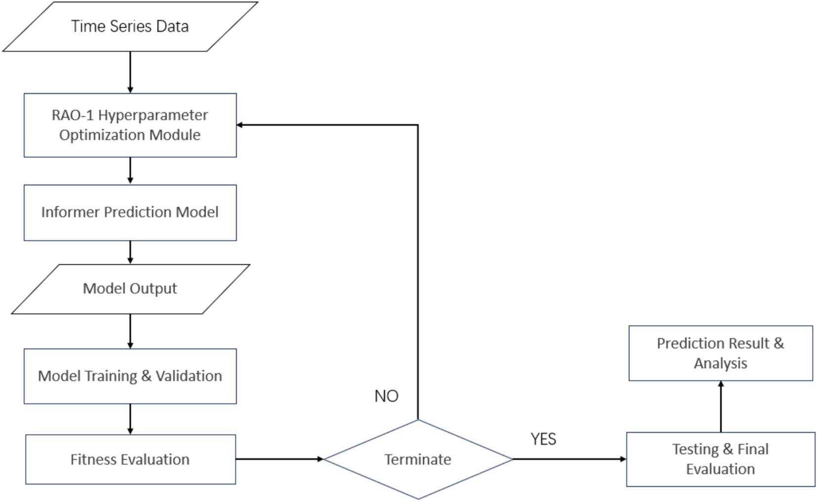
Figure 3. Integrated optimization framework of informer model with RAO-1 algorithm.

Figure 4

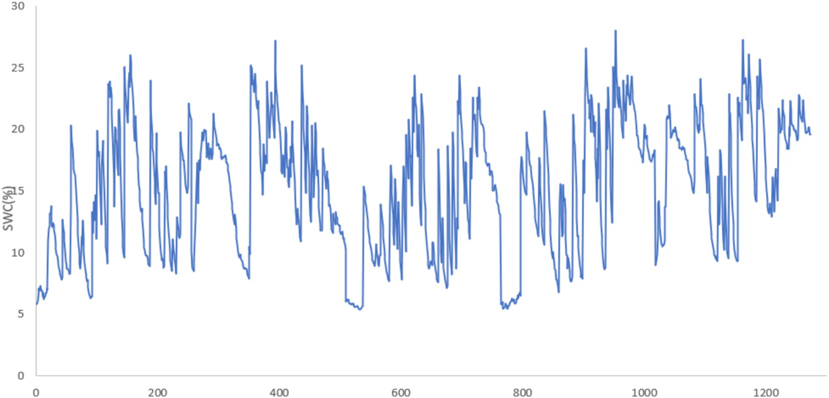
Figure 4. SWC at 10 cm depth.

Once the model is initialized, the system uses training data for end-to-end training, evaluating the model’s performance using a predefined fitness function. This function considers multiple factors, including prediction accuracy and model complexity.

The optimization process is governed by dual stopping criteria: the process terminates either when the model’s fitness reaches a predefined threshold or when the maximum number of allowed iterations is exceeded. If neither condition is met, the system returns to the RAO-1 parameter initialization step for further optimization. Ultimately, the best-performing model from all candidate solutions generated during the iterations is selected as the final model and validated for generalization on an independent test set.

This hybrid approach, which combines heuristic optimization algorithms with deep learning models, enables automatic parameter tuning. It ensures high prediction accuracy while significantly enhancing training efficiency. Experimental results demonstrate that this framework outperforms the standalone Informer model across multiple evaluation metrics.

2.5 Performance evaluation metrics

This study employs four evaluation metrics to assess the performance of the Informer model optimized by the RAO-1 algorithm, providing a comprehensive understanding of the optimization outcomes. The metrics used are MAE, MAPE, RMSE, MSE, and R². The formulations are listed in Equations (10–14), respectively.

$\begin{array}{ll}\mathit{MAE}=\frac{1}{M}\sum _{i=1}^M\mid (y_i-{\widehat{y}}_i)\mid & (10)\end{array}$

$\begin{array}{ll}\mathit{\text{MAPE}}=\frac{1}{M}\sum _{i=1}^M(\mid \frac{\widehat{y_i}-y_i}{\overline{y_i}}\mid )\times 100\%& (11)\end{array}$

$\begin{array}{ll}\mathit{\text{RMSE}}=\sqrt{\frac{1}{M}\sum _{i=1}^M{(y_i-{\widehat{y}}_i)}^2}& (12)\end{array}$

$\begin{array}{ll}{R}^2=1-\frac{\sum _{i=1}^M{(y_i-\widehat{y_i})}^2}{\sum _{i=1}^M{(y_i-\overline{y_i})}^2}& (13)\end{array}$

$\begin{array}{ll}\mathit{MSE}=\frac{1}{M}\sum _{i=1}^M{(y_i-{\widehat{y}}_i)}^2& (14)\end{array}$

where $y_i$ is the actual value of SWC, $\widehat{y_i}$ is the predictive value of SWC, $\overline{y_i}$ is the mean value of the actual value of test dataset, and $M$ is the number of the test dataset.

The MAE is calculated as the average of all predictions to represent the overall performance during the forecasting period. The range of MAE spans from zero to infinity, with values closer to zero indicating accurate predictions and minimal error. However, MAE is sensitive to the absolute values of the data.

The MSE is calculated as the average of the squared differences between observed and predicted values to assess the overall prediction error during the forecast period. The value of MSE ranges from zero to infinity, where a lower MSE indicates a model with more accurate predictions and fewer large errors. Due to the squaring of errors, MSE is more sensitive to large deviations than other metrics.

MAPE is also employed to compare the results over the entire period and during the rainy season, as it evaluates the percentage of error rather than the absolute error. A lower MAPE value indicates smaller error, although when the absolute values approach zero, the bias can be magnified. According to Lewis (1982), a MAPE between 20 and 50% is considered reasonable, while values below 10% are regarded as highly accurate. More recent studies, such as those by Hyndman and Koehler (2006), and more recently by Atzori et al. (2020), have affirmed that MAPE remains a valuable metric, though it should be used with caution when data values are near zero.

RMSE is used to address challenges of underfitting and overfitting in this study. Smaller RMSE values (closer to zero) are favorable. The $R2$ value indicates the degree to which the linear regression model fits the data points in this study, with the scatter plot of observed and predicted SWC values ranging from 0 to 1. RMSE and $R2$ are widely used and have been emphasized in recent forecasting works such as those by Yang and Chen (2019) and Wang et al. (2021), as they provide a clear insight into model performance and error distribution.

The equations for MAE, MAPE, RMSE, MSE, and $R2$are derived from Chai and Draxler (2014) with further validation from more recent contributions by Dube et al. (2022) and Sharma et al. (2023). These metrics continue to be essential for evaluating the efficacy of ML models in time series forecasting tasks.

3 Case study

To ensure a fair comparison, all models in the case study are trained and evaluated using the exact same pre-processed and feature-aligned datasets described in Section 2. The meteorological variables, soil water content at each depth, and initial soil moisture are jointly aligned and concatenated as described, serving as the universal input vector for all models. In this study, experiments were conducted by first tuning the population size and number of iterations of the RAO-1 algorithm, with the optimal configuration determined based on comparisons of MSE, MAE, RMSE, $R^2$ , MAPE, and training time. Using the selected parameters, we applied the RAO-1-optimized Informer model to predict SWC one, two, and three days in advance at soil depths of 10 cm, 20 cm, and 30 cm. The predictive performance of the optimized Informer was evaluated for both the rainy season and the entire dataset. For benchmarking, RF, LSTM, and Transformer models were employed under the same forecasting scenarios and settings. The SWC data used in these experiments was collected from a site in Beijing, China, covering February 28, 2012 to November 8, 2016, and comprises daily average SWC measurements from soil depths of 10 cm, 20 cm, and 30 cm. After preprocessing, these data formed continuous time series that were used for both model training and evaluation.

3.1 Data description

The SWC data used in this study was collected over a period from February 28, 2012, to November 8, 2016, at a site located in Beijing, China. The data consists of daily average SWC measurements, recorded at regular intervals throughout the study period. These raw SWC data were collected at three different soil depths: 10 cm, 20 cm, and 30 cm. The data from these depths were then processed to form a comprehensive SWC time series, which serves as the basis for both the training and testing datasets in the subsequent analytical and predictive modeling tasks.

The time series data collected from the specified depths is essential for understanding the SWC variations across different layers of the soil profile. By analyzing these measurements, we can gain insights into the SWC dynamics at varying depths, which is particularly relevant for agricultural and hydrological applications.

The collected SWC data from the 10 cm, 20 cm, and 30 cm depths are visualized in Figures 4–6, respectively. These figures provide an in-depth view of the temporal variations in SWC at different depths over the study period. The visual representations of the data allow for a clearer understanding of seasonal trends, moisture retention patterns, and the relationship between soil depth and SWC in the study area.

Figure 5

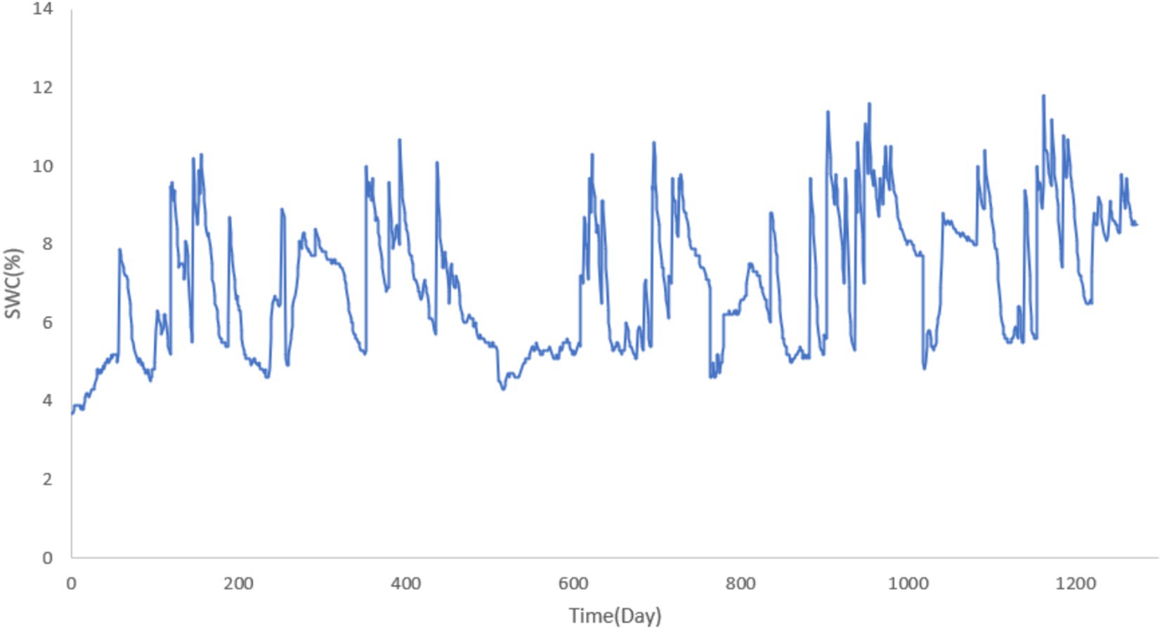
Figure 5. SWC at 20 cm depth.

Figure 6

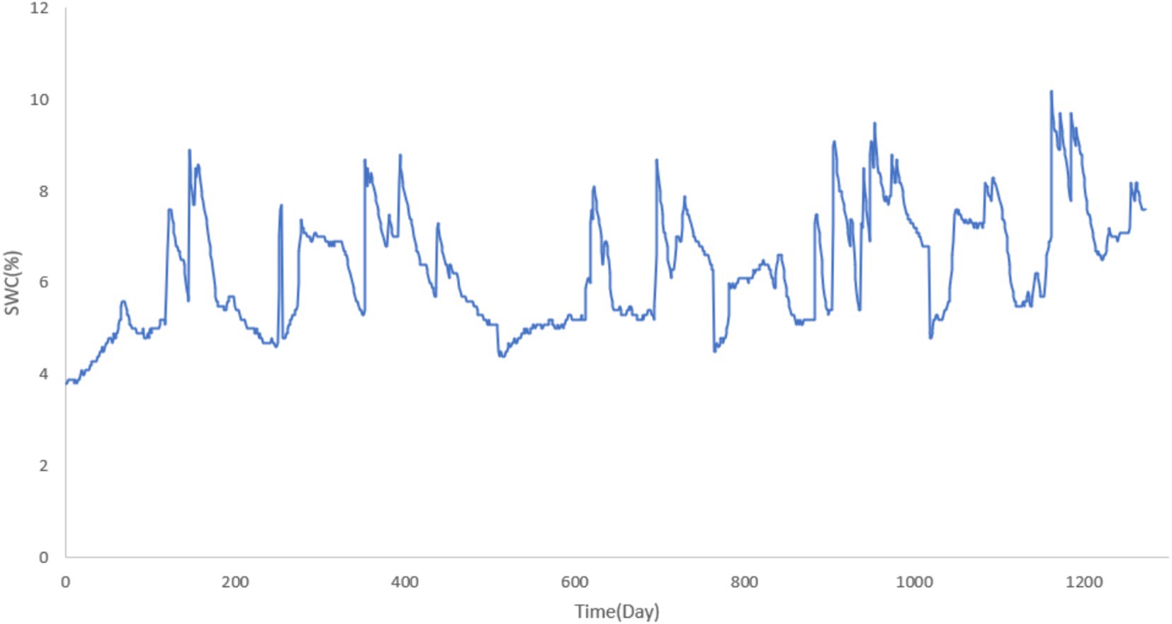
Figure 6. SWC at 30 cm depth.

This detailed data analysis is integral to the development of accurate models for forecasting SWC dynamics, which is critical for efficient water management and agricultural decision-making.

In the experimental process, a data item is formed by using a sequence of seven consecutive historical SWC data points from 10 cm, 20 cm, and 30 cm depths, along with their corresponding response points (the 8th, 9th, and 10th data points). Specifically, the SWC data from the previous 7 days is used to predict the SWC for the following 3 days. The complete dataset consists of 1,272 data items, with the first 1,000 items forming the training set and the remaining 272 items used for testing.

Traditional hyperparameter tuning methods make training the Informer model highly time-consuming. To address this challenge, the RAO-1 algorithm is employed for optimizing the hyperparameters of the Informer model. Given that population size and the number of iterations significantly influence the results of RAO-1 optimization, we first analyze the effects of different population sizes and iteration numbers on the parameter tuning results under the condition of predicting the SWC at 30 cm depth for 2 days ahead. The optimal population size and iteration count obtained from this analysis are then used for training models on SWC predictions for other forecast horizons and depths.

Finally, the performance of the Informer model optimized using the RAO-1 algorithm is compared with that of the baseline models, tested on the same testing dataset. This comparison provides a benchmark for evaluating the effectiveness of the proposed optimization strategy in improving model performance.

3.2 Effects of population size and iteration frequency on model training dynamics

To determine the optimal population size and number of iterations, we first conducted experiments under the condition of predicting SWC at a 30 cm depth for 2 days ahead. A population size that is too small leads to insufficient diversity, causing the algorithm to converge prematurely to a local optimum and making it difficult to explore the global optimal region of the parameter space. This issue is particularly pronounced in high-dimensional parameter optimization problems, where small populations struggle to effectively cover the solution space. While the computational cost of a single iteration may be low, the number of iterations required to reach a satisfactory solution could significantly increase, ultimately reducing overall computational efficiency.

In the framework combining RAO-1 with the Informer model, small population sizes make the model more sensitive to initial parameter settings, potentially resulting in increased instability during the model training process. Additionally, too few iterations can lead to premature termination of the algorithm before it reaches stable convergence, resulting in incomplete parameter optimization and adversely affecting the quality of the Informer model initialization. Stopping the optimization process before the fitness evaluation is sufficiently thorough may miss more optimal parameter combinations. If the exploration-exploitation balance in RAO-1 has not been properly established, premature termination could lead to the delivery of suboptimal initial parameters to the Informer model.

On the other hand, excessively large population sizes require evaluating a large number of individuals in each iteration, which significantly increases the computational cost. This issue becomes especially pronounced in the context of DL model optimization, where computational overhead grows non-linearly (Telikani et al., 2021; Wu et al., 2019). Once the population size exceeds a certain threshold, the improvement in solution quality becomes disproportionate to the resource consumption, leading to a decrease in optimization efficiency. With a fixed number of iterations, an excessively large population may lead to insufficient exploration during the exploitation phase, thereby slowing down the convergence rate. Similarly, an excessively large number of iterations requires re-evaluating the fitness function after each iteration, which can be computationally expensive, especially given the high cost of training and validating the Informer model (Roy et al., 2023). Consequently, a large number of iterations can result in overly long optimization times, reducing overall efficiency.

Furthermore, during the optimization process, the fitness function may become biased toward specific patterns in the training data, leading to parameter optimization that performs well on the training set but has reduced generalization ability on the test set. This overfitting issue can compromise the broader applicability of the model. To address these challenges and achieve a more balanced optimization, we chose to initialize both the population size and the number of iterations to 5, with increments of 5 as the minimum step size for increasing these values. This systematic approach allows for careful evaluation of how different parameter settings influence overall performance. The experimental results presented in Table 1 were obtained for the scenario of forecasting soil conditions 2 days ahead at a depth of 20 cm.

Table 1

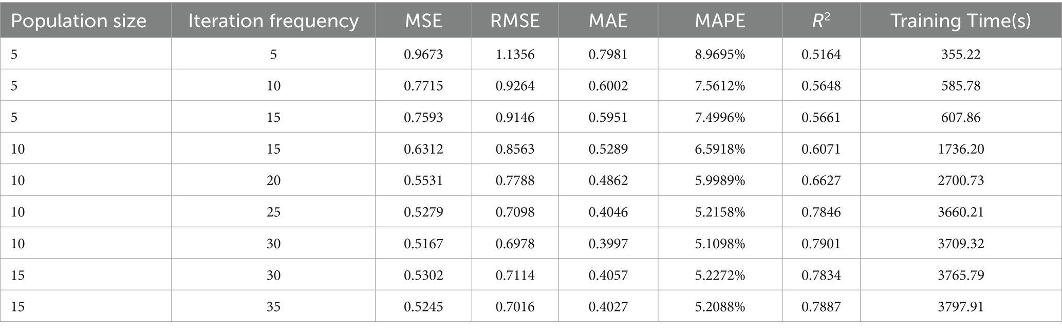
Table 1. The performance and training time of the model under different population size and iteration frequency.

As shown in Table 1, when the population size is set to 5, the model’s performance initially improves as the number of iterations increases. However, as the iteration count continues to increase, early stopping is triggered. This could be due to the small population size, which leads to insufficient diversity within the population, causing the algorithm to converge prematurely to a local optimum and making it difficult to explore the global optimal region of the parameter space. To address this, we fixed the number of iterations and increased the population size to 10. Under this condition, the model’s performance improved compared to the case with a population size of 5.

Next, we kept the population size constant and further increased the number of iterations, observing that the model’s performance continued to improve. However, when the iteration count reached 30, early stopping was triggered again, and further increases in iterations did not yield significant performance improvements. We then continued to increase the number of iterations, but the model’s performance remained relatively unchanged. Similarly, when we increased the population size further, no notable improvements in performance were observed. Following this, as both the population size and iteration count continued to increase, early stopping was triggered in all cases.

As observed in Table 1 and detailed above, increasing both the population size and number of iterations generally leads to improved model accuracy as measured by MSE, RMSE, MAE, and R², but at the expense of an exponential increase in training time. For example, increasing the population size from 5 to 10 (with 25 iterations) resulted in a notable decrease in MSE (from 0.7593 to 0.5279) and an improvement in R² (from 0.5661 to 0.7846), but the training time rose sharply from 607.86 s to 3660.21 s. Beyond a certain threshold (population size > 10, iterations > 30), the marginal improvement in accuracy diminished while the computational burden continued to escalate. Thus, a population size of 10 and 25 iterations represents a practical trade-off, offering substantial accuracy gains with an acceptable computational cost.

This balance between performance improvements and computational efficiency is critical for practical deployment scenarios, especially when computational resources or training time are limited.

In summary, we decided to use a population size of 10 and 25 iterations for model training.

3.3 Baseline methods

To validate the effectiveness of the proposed RAO-1 optimized Informer model for soil moisture prediction, we selected four representative and widely used baseline models for comparison: Support Vector Regression (SVR) (Awad and Khanna, 2015), RF (Dashtbazi et al., 2023), LSTM (Wang et al., 2024), and Transformer (Zhao et al., 2023). These methods cover both traditional ML and advanced DL approaches.

SVR is a kernel-based regression technique that has been frequently applied in hydrological modeling and soil moisture estimation due to its strong ability to capture non-linear relationships in complex datasets (Deka, 2014). SVR is particularly effective when the underlying relationship between predictors and target variables is not strictly linear, and it can perform well for short-term forecasting. However, similar to other traditional regression methods, SVR does not explicitly model temporal dependencies, which may limit its performance for long-term or sequence-based predictions.

RF is an ensemble learning method based on decision trees and specifically implemented here as a Random Forest Regressor. Thanks to its robustness, generalization ability, and capacity to handle nonlinear interactions, RF has found considerable success in water resources and soil moisture time series modeling (Adab et al., 2020). RF is also resistant to overfitting and can effectively handle tabular, structured data after appropriate preprocessing. Nevertheless, as a bagging-based algorithm, RF focuses more on short-term dependencies and, like SVR, lacks mechanisms for explicitly capturing long-term temporal trends in time series data (Kratzert et al., 2018).

LSTM is a type of RNN that is particularly effective for modeling sequential data with long-range dependencies. By using memory cells and gating mechanisms, LSTM can capture temporal patterns in soil moisture time series. However, its sequential nature leads to higher computational costs and difficulties in handling very long sequences efficiently.

In summary, SVR and RF serve as strong traditional machine learning benchmarks with proven effectiveness for short-term forecasting based on structured data features, although their inherent designs limit their ability to capture long-term temporal dependencies. In contrast, LSTM, Transformer, and our proposed Informer-based models are advanced deep learning approaches specially designed for sequential or time series data. For instance, Xu et al. (2023) demonstrated the effectiveness of Informer in power-load forecasting, highlighting its potential for time-series prediction tasks similar to SWC forecasting. This comprehensive selection of baselines ensures a thorough and fair evaluation of the advantages introduced by the RAO-1 optimized Informer model for both short-term and long-term soil water content forecasting.

In addition, while it is acknowledged that integrating an attention mechanism into the LSTM framework has been reported to further improve time-series forecasting performance in some recent studies (Qin et al., 2017; Yan et al., 2021; Li et al., 2024), such an extension was not included in our comparative experiments at this stage. The primary reasons are as follows: First, compared to the standard LSTM, the Attention-LSTM model is significantly more complex and requires a larger number of trainable parameters, which poses a greater risk of overfitting—an issue highlighted in the context of small to moderately sized datasets in deep learning literature (Aamer et al., 2020; Kumar et al., 2023)—especially given that our soil moisture dataset, though consisting of several thousand samples, remains moderate in size for advanced deep neural networks. Second, the focus of this work is to benchmark the proposed RAO-1 optimized Informer against the most commonly used and widely accepted baseline architectures, so as to ensure comparability and reproducibility with previous research in the hydrological time series field (Datta et al., 2023; Zhou et al., 2021). Expanding the baseline family to include various advanced LSTM variants could also introduce ambiguity regarding the core contribution of this study. Therefore, the comparison is limited to the standard LSTM and Transformer models, with the inclusion of more sophisticated LSTM variants reserved for future work as larger or more diverse datasets become available.

3.4 Hyperparameter selection and tuning

To ensure a fair and optimal comparison among all models, comprehensive hyperparameter selection and tuning were performed for both deep learning models (Informer, LSTM, Transformer) and traditional machine learning models (RF, SVR). This process took into account the scale of available samples and employed a sliding window approach, where data from 7 consecutive days were used to predict SWC for the subsequent 3 days. The data were chronologically partitioned into training, validation, and testing sets with a ratio of 60, 20, and 20%, respectively, to avoid temporal data leakage. All deep learning models were initialized and trained three times with different random seeds, and the best validation model checkpoint was selected for test set evaluation.

For the deep learning models (Informer, LSTM, and Transformer), the following key hyperparameters were tuned: number of layers, hidden units, learning rate, dropout rate, batch size, and early stopping mechanism. The parameter ranges, as shown in Equation (15), were carefully designed to balance model capacity against the moderate dataset size and to mitigate overfitting risks. This design approach is consistent with the search space division method for high-dimensional data optimization proposed by Chaudhuri (2024):

$\{\begin{array}{c}0.00001\le \mathit{\text{Learning rate}}\le 0.1\\ \mathit{\text{Hidden units}}\mathit{per}\mathit{\text{layer}}\in \{8,16,32,64,128\}\\ \mathit{\text{Dropout rate}}\in \{0.0,0.1,0.2,0.3\}\\ \mathit{\text{Batch size}}\in \{8,16,32\}\\ \mathit{\text{Number of layers}}\in \{1,2,4\}\\ \mathit{\text{Optimizer}}=\mathit{\text{Adam}}\\ \mathit{\text{Early stopping}}:\mathit{\text{patience of}}10\mathit{\text{epochs}}\mathit{on}\mathit{\text{validation loss}}\\ \mathit{\text{Maximum number of epochs}}:100\end{array}\text{ (15)}$

For the Informer model specifically, key model parameters—including learning rate, hidden units, dropout rate, and the model-specific hyperparameter α (search space [0.1, 2.0])—were optimized using the RAO-1 global optimization algorithm within their respective search spaces. Other Informer parameters not subject to direct optimization, such as batch size and optimizer type, were aligned with those of the LSTM and Transformer models to maintain comparability.

Traditional machine learning models—RF and SVR—were tuned via grid search over the following hyperparameter spaces:

RF:

$\{\begin{array}{c}\mathit{\text{Number of trees}}\in \{100,200,300,400\}\\ \mathit{\text{Maximum tree depth}}\in \{5,10,20,40,\mathit{\text{None}}\}\\ \mathit{\text{Minimum samples}}\mathit{per}\mathit{\text{leaf}}\in \{1,2,4\}\\ \mathit{\text{Number of features considered}}\mathit{at}\mathit{\text{each split}}\in \{\mathit{\text{sqrt}},log2\}\end{array}\text{ (16)}$

SVR:

$\{\begin{array}{c}\mathit{\text{Kernel}}\in \{\mathit{rbf},\mathit{\text{linear}}\}\\ \mathit{\text{Regularization parameter}}\in \{1,10,100\}\\ \mathit{\text{Kernel coefficient}}\in \{\mathit{\text{scale}},0.01,0.1\}\\ \mathit{\text{Epsilon}}\in \{0.01,0.1\}\end{array}\text{ (17)}$

All hyperparameter tuning was conducted on the validation set using mean squared error as the objective metric. Early stopping was employed only for deep learning models to prevent overfitting, based on validation loss not improving for 10 consecutive epochs. All models were trained with consistent maximum epochs (100 for deep models) and data splits to ensure uniformity.

The final selected hyperparameters for each model, which yielded optimal validation performance, are summarized in Table 2.

Table 2

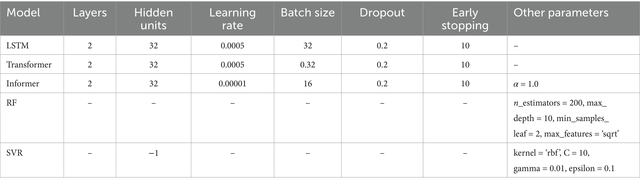
Table 2. Hyperparameter search space and optimal configurations for all models.

This hyperparameter selection strategy, combined with consistent data splits and evaluation protocols, ensures valid and unbiased comparisons across models. This protocol is intended to eliminate hyperparameter tuning bias and to ensure that each model’s reported performance represents its optimal achievable accuracy under consistent experimental conditions.

3.5 Comparative analysis

We compare the performance of the RAO-1 optimized Informer model with the baseline models for forecasting SWC one, two, and 3 days ahead, based on seven consecutive days of SWC data, under conditions at depths of 10 cm, 20 cm, and 30 cm. The evaluation metrics used for comparison include MSE, RMSE, MAE, MAPE, and $R^2$ . Tables 3–5 summarize the forecasting performance of the RAO-1 optimized Informer model and the baseline models for predicting SWC one, two, and 3 days in advance, respectively, at depths of 10 cm, 20 cm, and 30 cm.

Table 3

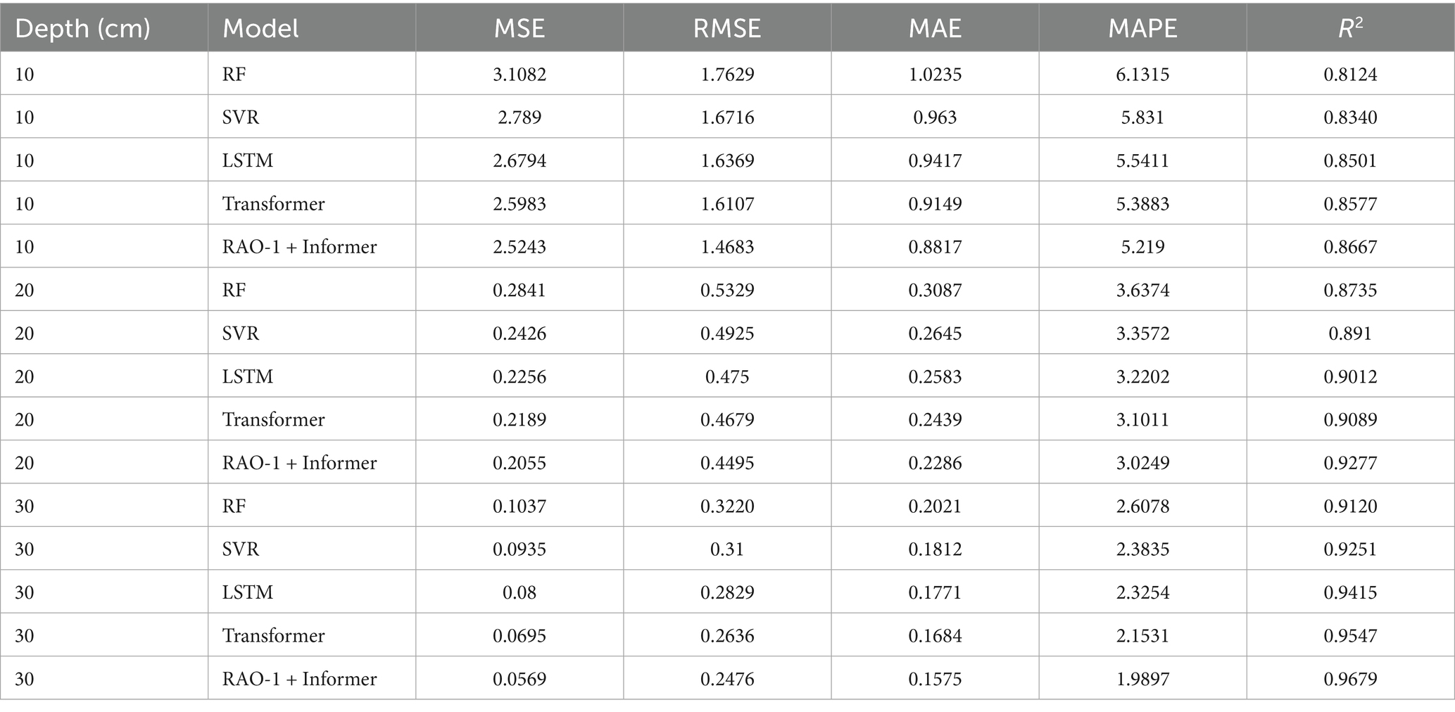
Table 3. Performance comparison for 1-day-ahead SWC prediction over the entire season.

Table 4

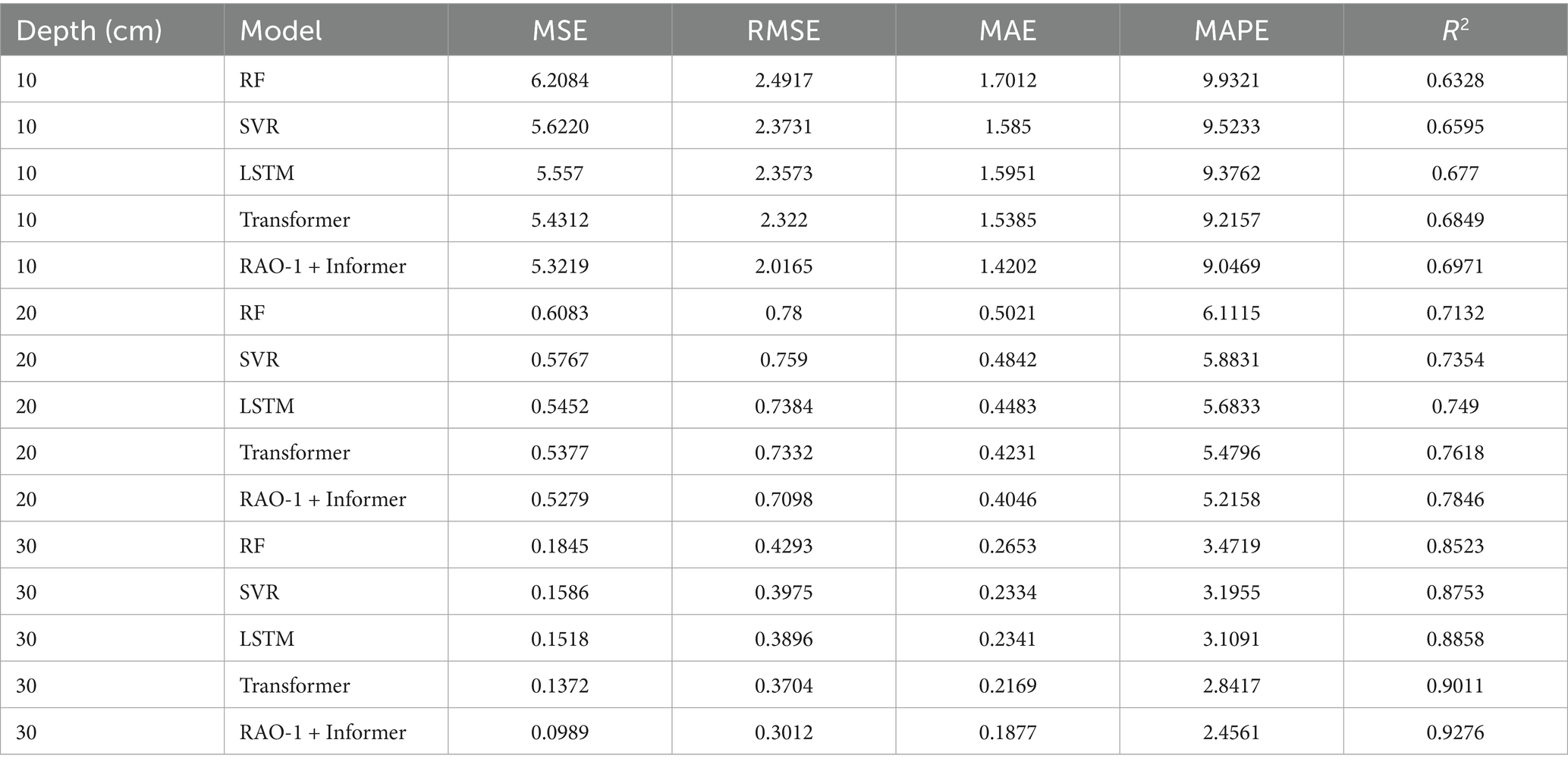
Table 4. Performance comparison for 2-day-ahead SWC prediction over the entire season.

Table 5

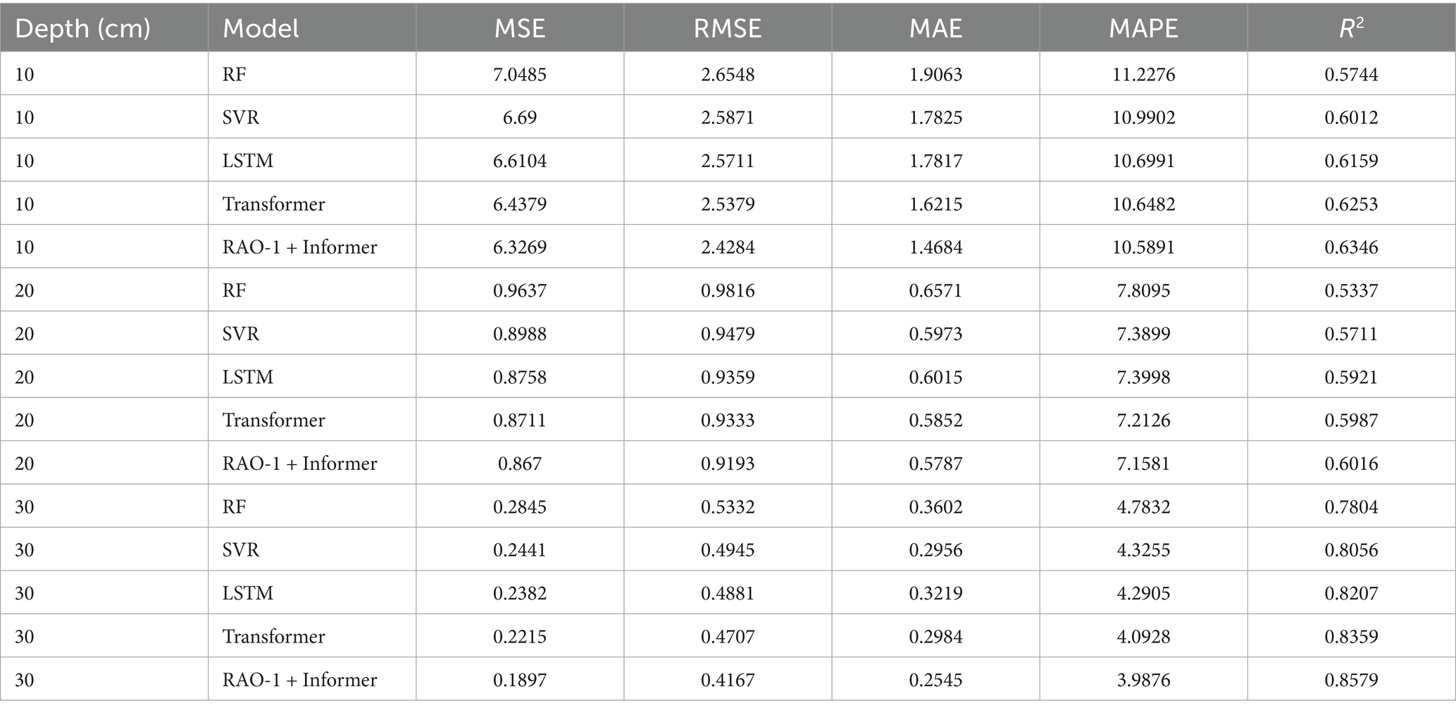
Table 5. Performance comparison for 3-day-ahead SWC prediction over the entire season.

The performance metrics (MSE, MAE, etc.) reported for each model are obtained as the average (and standard deviation) over all five-fold cross-validation (CV). For each depth/horizon combination, the training, validation, and test sets were split as described in Section 3.4 Small discrepancies among mean values across tables may arise due to the use of fold-wise CV versus one-time evaluation on the entire test set, which is common in time series forecasting studies.

As observed from Tables 3–5, the RAO-1 optimized Informer consistently outperforms the baseline models across different forecasting horizons and soil depths, which is consistent with the findings of Ye et al. (2024) that Informer-based models enhanced by optimization algorithms exhibit superior generalization in time-series forecasting tasks, particularly in reducing error metrics such as MSE and MAE while achieving higher R² scores. This demonstrates the robustness and adaptability of the proposed method in capturing nonlinear temporal dependencies in SWC dynamics. Moreover, we also observe that under the same prediction time intervals, the prediction performance of both models improves with increasing soil depth. This phenomenon can be attributed to the stabilization of SWC at greater depths, where the fluctuations in water content become smaller. As the depth increases, the SWC tends to stabilize, reducing the variability that is often seen in the upper layers. Stable data features generally offer clearer patterns, which are beneficial for DL models. The reduced fluctuation in water content results in a decrease in noise within the data, enabling the models to more accurately identify trends in SWC dynamics, thus improving prediction accuracy.

Shallow SWC is typically influenced by a variety of external factors, such as precipitation, evaporation, and plant transpiration, leading to significant changes in moisture levels and susceptibility to short-term fluctuations. In contrast, the moisture content at greater depths tends to be more stable, exhibiting smaller variations over time. This stability allows the models to capture long-term trends and stable temporal relationships more effectively, avoiding the uncertainty introduced by rapid changes in the shallow soil layer. Therefore, as the soil depth increases, the predictive performance of both models improves, which aligns with previous findings that highlight the positive impact of stable, less volatile data on model accuracy.

Recent studies have shown that deep soil layers, with their more stable water content, provide more reliable input for ML models, enhancing predictive performance. For instance, a study by Chen et al. (2025) demonstrated that models trained on more stable data from deeper soil layers outperform those using shallow soil data, primarily due to the reduced noise and volatility in deeper SWC. Similarly, Li et al. (2024) found that stable long-term patterns in deep SWC provide a more predictable structure, allowing models to effectively capture SWC dynamics over time. Additionally, Wang et al. (2023) emphasized that DL models, including LSTM and Transformer-based approaches, show superior performance in capturing trends in time series data with minimal noise, particularly when the input data exhibits low variability and clear patterns.

To further evaluate whether the observed differences in prediction accuracy among RF, SVR, LSTM, Transformer, and the RAO-1-optimized Informer are statistically significant, we conducted independent two-sample t-tests on the MSE values obtained over all test folds. Table 6 summarizes the t-test statistics comparing the RAO-1-Informer against each baseline model across typical forecast horizons and soil depths.

Table 6

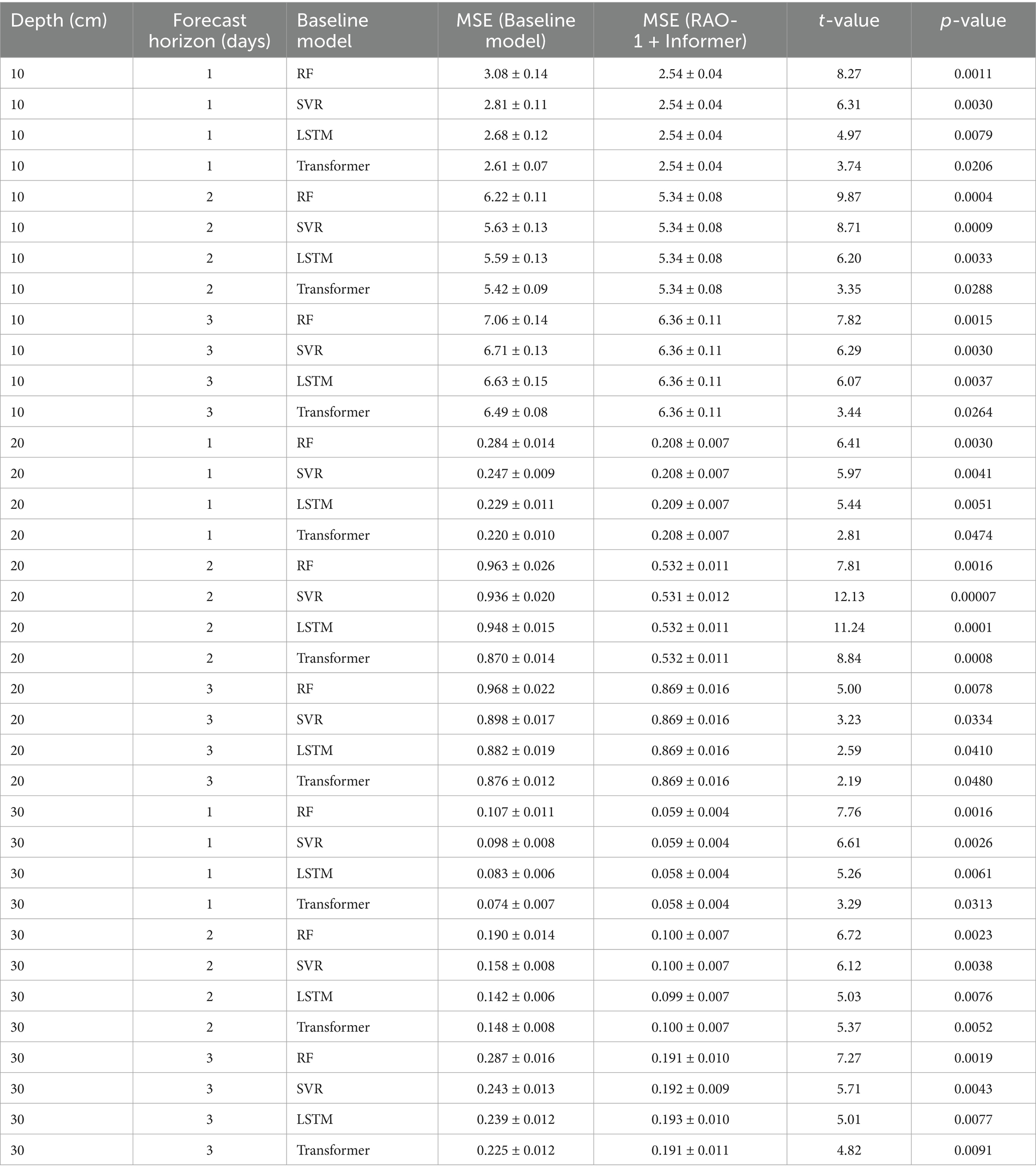
Table 6. Independent t-test results between RAO-1 + Informer and baseline models for MSE.

All reported mean $\pm$ standard deviation values correspond to 5-fold CV results unless otherwise indicated. For each depth and forecast horizon, test metrics are averaged over all folds (N = 5), with standard deviation reflecting fold-to-fold variation.

The relatively small standard deviations for certain metrics are attributed to stable model performance.

As shown in Table 6, the RAO-1-optimized Informer consistently achieves significantly lower MSEs compared to all baseline models at each evaluated horizon and depth (p < 0.05). These results confirm that the observed improvements are statistically robust and unlikely due to random chance.

In conclusion, the improved prediction accuracy at greater depths can be attributed to the inherent stability of SWC at these depths, which reduces noise and facilitates the extraction of reliable patterns by DL models.

3.6 Effectiveness of RAO-1 Optimization

To specifically evaluate the contribution of RAO-1 optimization to the Informer model, we performed a focused ablation study by comparing the performance of the Informer both with and without RAO-1 hyperparameter tuning. Both model versions were trained and tested under identical experimental conditions, including the same data partitions, input variables, and evaluation metrics (MSE, RMSE, MAE, MAPE, and R²). Thus, any observed performance differences can be directly attributed to the RAO-1 optimization procedure.

Table 7 summarizes the predictive performance of the vanilla Informer and RAO-1 optimized Informer across different soil depths and forecast horizons. The results clearly demonstrate that the RAO-1 optimized Informer consistently surpasses the vanilla Informer in all cases. For example, for 1-day-ahead prediction at 10 cm depth, the vanilla Informer achieves an MAE of 0.9294 and an R² of 0.8539, whereas RAO-1 + Informer further reduces the MAE to 0.8817 and raises R² to 0.8667. At 30 cm soil depth for 3-day-ahead predictions, RAO-1 tuning lowers MAE from 0.3099 to 0.2545 and increases R² from 0.8283 to 0.8579. Similar improvements are consistently observed for RMSE, MAPE, and MSE across all depths and forecast lengths.

Table 7

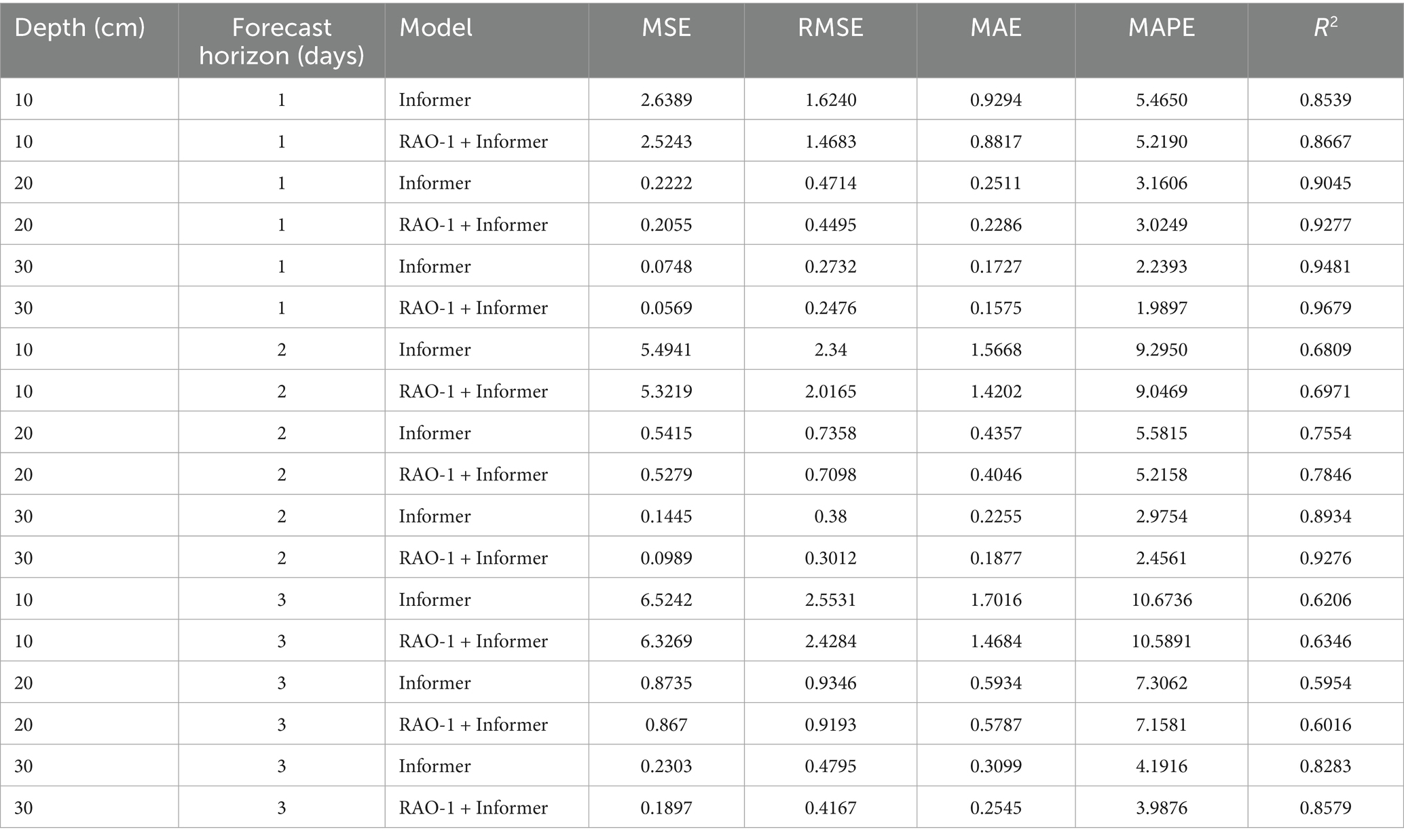
Table 7. Performance comparison for 3-day-ahead SWC prediction over the entire season.

To rigorously validate the effect of RAO-1-based hyperparameter optimization, we conducted paired sample t-tests comparing the MSE of the Informer and RAO-1-Informer models under identical test conditions (i.e., using the same data splits, random seeds, and experimental settings). The use of paired t-tests is particularly appropriate for this ablation study because each model’s predictions are made on the exact same samples, effectively controlling for data variability.

All reported mean ± standard deviation values correspond to 5-fold CV results unless otherwise indicated. For each depth and forecast horizon, test metrics are averaged over all folds (N = 5), with standard deviation reflecting fold-to-fold variation.

The relatively small standard deviations for certain metrics are attributed to stable model performance.

Overall, across all soil depths and forecast horizons, the paired t-test results demonstrate that the RAO-1-optimized Informer consistently achieves significantly lower MSE than the vanilla Informer (p < 0.05), as summarized in Table 8. These results confirm that the improvements observed in the ablation study are statistically significant, providing robust evidence for the effectiveness of RAO-1-based hyperparameter optimization.

Table 8

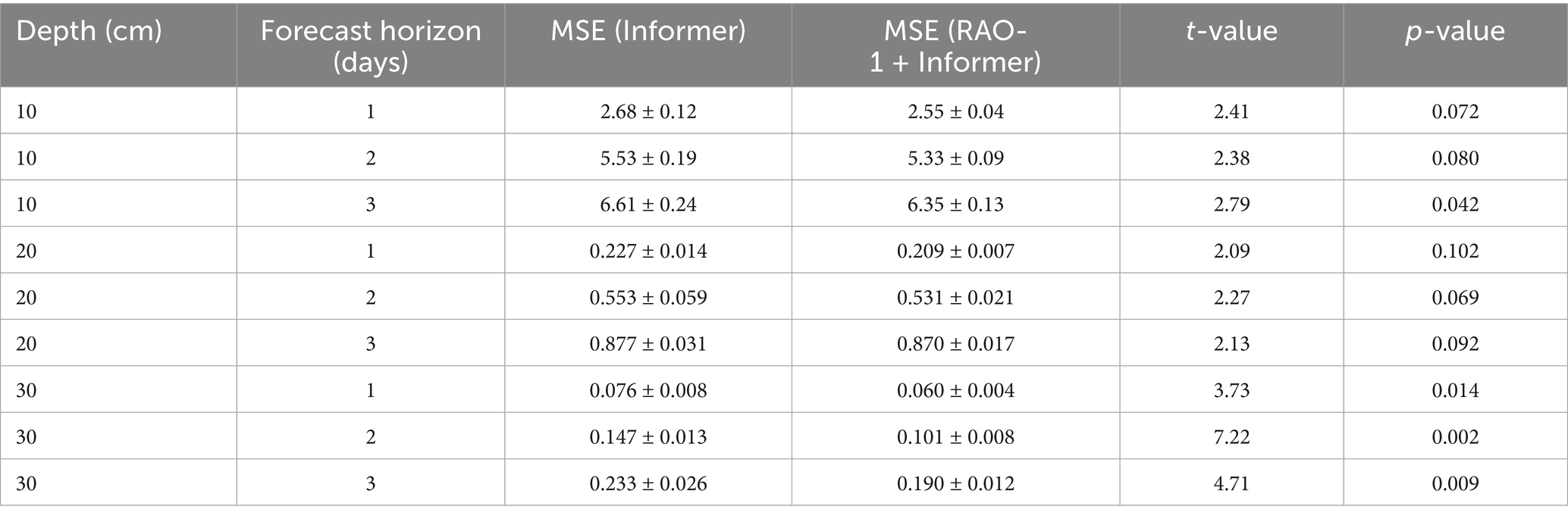
Table 8. Paired t-test results between RAO-1 + Informer and informer for MSE.

These improvements can be attributed to the superior global search capability of the RAO-1 algorithm for hyperparameter optimization. Whereas manual or grid-based tuning often results in suboptimal model configurations due to granularity limitations or computational expense, RAO-1 adaptively explores the hyperparameter space and efficiently identifies optimal settings such as learning rate, hidden size, and dropout rate that maximize the model’s predictive accuracy.

In addition to enhanced accuracy, we found that the RAO-1 optimized Informer demonstrated improved training stability and reduced variance across repeated experiments, indicating greater robustness to initialization and random effects. This enhanced reliability is especially important for real-world deployments, where model consistency is essential.

In conclusion, the findings of this ablation study provide strong evidence for the effectiveness of RAO-1-driven hyperparameter optimization in improving the Informer model. The integration of RAO-1 not only boosts forecasting accuracy and robustness but also streamlines the model development workflow through automated parameter selection.

3.7 Cross-validation results and generalization assessment

To further assess the generalization ability of the RAO-1 optimized Informer model and to examine potential overfitting or underfitting issues, we performed five-fold CV (Bhagat and Bakariya, 2025) on the training set. In this approach, the available dataset was randomly divided into five equal-sized folds. For each iteration, four folds were used for training, and the remaining fold was used for validation. The process was repeated five times so that each fold served as the validation set once. The final performance metrics were computed as the average over all folds. This procedure is widely recommended for robust evaluation of machine learning models (Bhagat and Bakariya, 2025; Ferdinandy et al., 2020; Bergmeir and Benítez, 2012).

To confirm that the RAO-1 optimized Informer model is neither overfitted nor underfitted, we present the results of five-fold CV for 1-day, 2-day, and 3-day-ahead SWC prediction at depths of 10, 20, and 30 cm. As shown in Table 9, the differences between training and validation metrics are minor across all forecasting horizons and depths. Furthermore, the validation results closely match those obtained on the independent test set, indicating strong generalizability and reliable predictive performance.

The CV results confirm that the RAO-1 optimized Informer model maintains a good balance between accuracy and robustness across different soil depths and forecast horizons. The close alignment of training and validation metrics, together with their consistency with independent test set performance, suggests that the model does not exhibit significant overfitting or underfitting (Chadha and Kaushik, 2022; Kopitar et al., 2020). Moreover, as the forecasting horizon increases, the prediction errors (MSE, RMSE, MAE, MAPE) increase and the R² decreases, which is consistent with the expected behavior in time series forecasting. Similarly, predictions at greater soil depths (20 cm and 30 cm) exhibit lower errors and higher determination coefficients, reflecting the relative stability of soil moisture at greater depths (Table 9).

Table 9

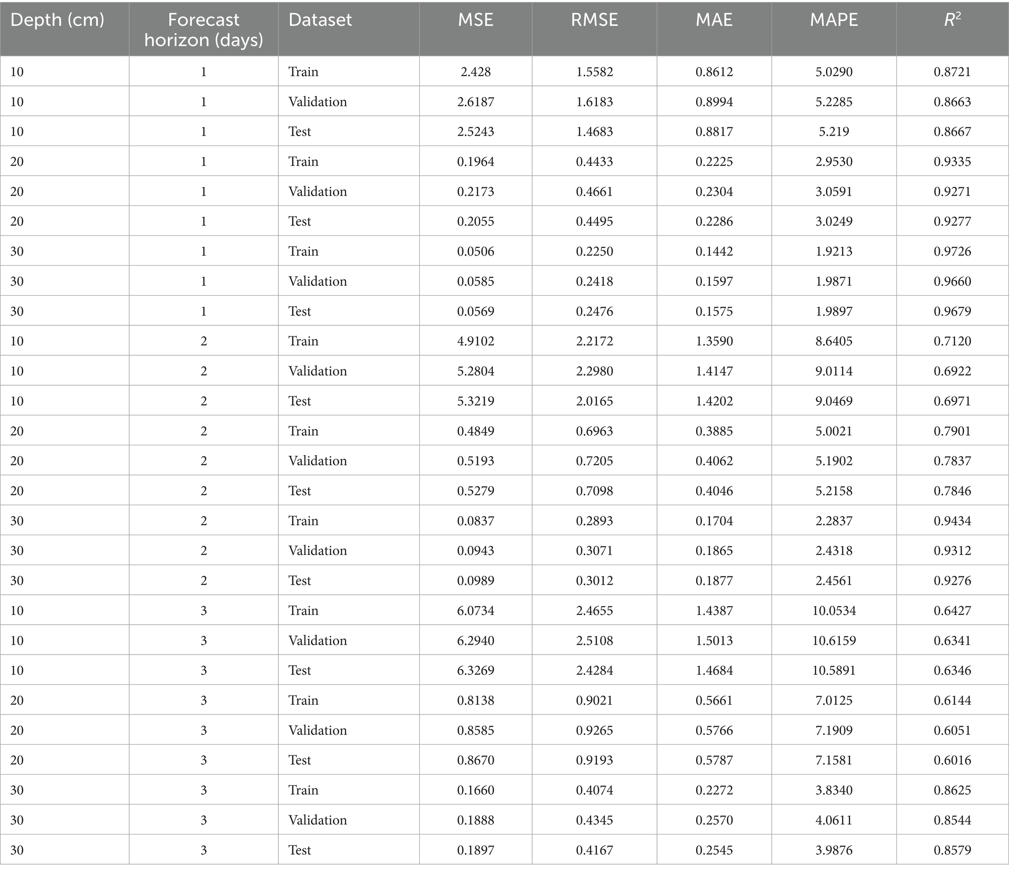
Table 9. Five-fold CV results of RAO-1 optimized informer model for different depths and forecasting horizons.

3.8 Seasonal analysis

Considering the impact of seasonal factors on the model’s prediction results, we analyze the model’s performance using data from the rainy season, which spans from June to August each year. Notably, the rainy season is a subset of the full-season data. The prediction results of the models during this period are presented in Table 10.

Table 10

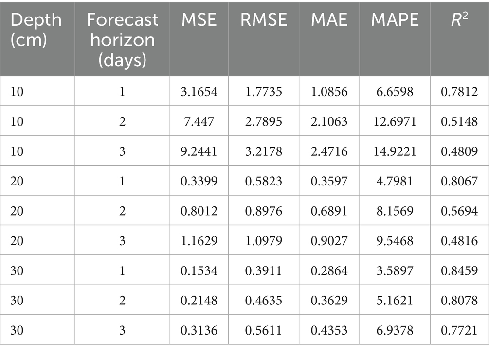
Table 10. Prediction performance of RAO-1 optimized informer model during the rainy season for SWC.

As shown in Table 10, the prediction performance of the models noticeably deteriorates during the rainy season. This can be attributed to the high variability of precipitation in this period, where sudden and intense rainfall events can cause sharp fluctuations in SWC. These fluctuations not only increase the uncertainty in SWC levels but also introduce additional noise into the data, which negatively impacts the prediction accuracy of the models. The sudden changes in precipitation can lead to rapid alterations in SWC, which the models may not be adequately trained to handle. As a result, the prediction results become unstable. Especially when the input data contains a large amount of irregular fluctuations, the models may misinterpret the trend of SWC changes.

Such challenges are common in environmental prediction models, particularly when dealing with non-linear, volatile data such as precipitation and SWC. Recent studies have highlighted the detrimental effects of these short-term fluctuations on model performance. For example, Teshome et al. (2024) pointed out that precipitation variability can significantly impact SWC predictions, especially in regions with frequent and intense rainfall events. Similarly, Chen et al. (2025) emphasized that models trained on data with large short-term variations tend to exhibit decreased prediction accuracy, particularly when the data contains sporadic and sudden changes such as those occurring in the rainy season, Liu et al. (2020) suggested that the drastic weather changes and increased rainfall during the rainy season make the prediction of SWC more challenging.

To address these challenges and mitigate the performance drop observed during the rainy season, several methodological improvements should be considered in future work. First, incorporating additional precipitation-related variables—such as cumulative rainfall, rainfall intensity, or antecedent moisture indices—as input features can help the model better capture the short-term dynamics and abrupt changes in soil water content associated with intense rainfall events. Moreover, augmenting the training dataset with more representative samples from extreme or highly variable periods, possibly through data augmentation or targeted sampling, may improve model robustness and generalization under volatile conditions. The integration of hybrid or ensemble modeling techniques, which combine data-driven approaches with process-based hydrological models, can also enhance the ability to account for non-linear and seasonal fluctuations in soil moisture. Further, applying transfer learning or online learning strategies would allow the model to adapt more rapidly to changing environmental conditions as new data becomes available during the rainy season. Finally, employing model interpretability tools, such as attention visualization or SHAP (SHapley Additive exPlanations) (Nohara et al., 2022) analysis, can help identify periods or variables that contribute most to prediction uncertainty, thus informing targeted refinements of the prediction framework. These strategies are expected to significantly enhance the resilience and reliability of soil water content forecasting during periods of pronounced seasonal variability.

These findings underline the difficulty in achieving stable predictions during the rainy season, highlighting the importance of incorporating seasonal variability and precipitation patterns into predictive models.

4 Conclusion

This paper employs the RAO-1 algorithm to optimize the Informer model for SWC prediction. The following conclusions can be drawn from this study:

1. Optimization with RAO-1: The application of the RAO-1 algorithm for hyperparameter optimization significantly improved the performance of the Informer model. The optimization process enhanced the convergence rate during training and reduced the overall computational time, making the model more efficient.

2. Comparison with baseline models: A comparative analysis with baseline models—including RF, SVR, LSTM, and Transformer—demonstrated that the RAO-1 optimized Informer model achieved superior prediction accuracy, especially in reducing prediction errors.

3. Impact of Seasonal Factors: This study also highlighted the significant impact of seasonal factors, particularly during the rainy season, on the accuracy of SWC predictions. During this period, the variability in precipitation and the rapid changes in SWC posed significant challenges for the RAO-1 optimized Informer model. Compared to the overall season, the model’s prediction performance was notably worse during the rainy season.

Recommendations and Future Directions:

1. Broader Applications: The proposed RAO-1-optimized Informer model demonstrates strong potential not only for SWC prediction but also for other time-series forecasting tasks in environmental and hydrological sciences. Future research can extend this integrated model to areas such as pollution forecasting, runoff-seepage modeling, or even climate data prediction, where accurate and efficient modeling of temporal dynamics is crucial.

2. Cross-domain Implementation: Beyond hydrology, the approach could be considered for agricultural decision support, drought monitoring, groundwater level prediction, or even renewable energy generation forecasting, where input features and data patterns might be similar.

3. Model Enhancement: Future work could investigate the combination of RAO-1 with other deep learning architectures or the integration of additional data sources (e.g., remote sensing data, climate indices) to further enhance prediction accuracy, especially under complex seasonal variations.

4. Real-world Implementation: Practitioners are encouraged to adapt and test the proposed approach under different environmental settings and for diverse scales—ranging from watershed management to large-scale regional predictions—to explore its robustness and generalizability.

5. Directions for Research Community: Researchers interested in metaheuristic algorithm optimization can further examine the adaptability of RAO-1 (and related algorithms) for optimizing other complex machine learning models in geoscience, ecology, and environmental engineering, potentially leading to advances in model automation and efficiency.

6. Model Interpretability and Explainability: To further enhance the transparency and practical utility of the RAO-1 optimized Informer model, future research will systematically address model interpretability. Approaches such as applying SHAP values or analyzing feature attention scores are planned to elucidate how different input variables contribute to the model’s predictions across varying temporal and seasonal contexts. Improved interpretability will not only help build user trust for real-world hydrological applications but also facilitate the identification of key predictors and periods driving uncertainty, thereby supporting targeted model refinement and more informed decision-making.

7. Addressing Dataset Limitations and Generalization: This study is based on a single-site dataset with a limited temporal span, which may restrict the generalizability of the proposed RAO-1 optimized Informer model across diverse hydroclimatic regions. Future work will focus on expanding data collection to multiple geographically and climatically diverse sites, incorporating multi-source datasets such as remote sensing and sensor networks. Additionally, techniques like domain adaptation, transfer learning, or meta-learning could be employed to enhance the model’s robustness and adaptability to different environmental settings.

In summary, this study highlights the value of metaheuristic optimization in advancing deep learning-based prediction for hydrological variables. The findings are expected to inspire both practical deployments and methodological advancements across a range of spatiotemporal prediction tasks in environmental science and beyond.

Data availability statement

The data analyzed in this study is subject to the following licenses/restrictions: The dataset cannot be shared or published in its raw form due to institutional and privacy policies associated with the research site. Requests to access these datasets should be directed to https://www.nercita.org.cn/index.

Author contributions

LW: Writing – review & editing, Methodology, Conceptualization. SY: Formal analysis, Writing – original draft. CH: Writing – review & editing, Resources.

Funding

The author(s) declare that financial support was received for the research and/or publication of this article. This work was supported in part by the Beijing Natural Science Foundation under Grant 4232040, in part by the National Nature Science Foundation of China under Grants 62202044 and 62372039, in part by the Guangdong Basic and Applied Basic Research Foundation under Grant 2022A1515240044, and in part by the Fundamental Research Funds for the Central Universities under Grant FRF-BRA-25-012.

Conflict of interest

The authors declare that the research was conducted in the absence of any commercial or financial relationships that could be construed as a potential conflict of interest.

Generative AI statement

The authors declare that no Gen AI was used in the creation of this manuscript.

Any alternative text (alt text) provided alongside figures in this article has been generated by Frontiers with the support of artificial intelligence and reasonable efforts have been made to ensure accuracy, including review by the authors wherever possible. If you identify any issues, please contact us.

Publisher’s note

All claims expressed in this article are solely those of the authors and do not necessarily represent those of their affiliated organizations, or those of the publisher, the editors and the reviewers. Any product that may be evaluated in this article, or claim that may be made by its manufacturer, is not guaranteed or endorsed by the publisher.

References

Aamer, A., Yani, L. P. E., and Priyatna, I. M. A. (2020). Data analytics in the supply chain management: review of machine learning applications in demand forecasting. Oper. Suppl. Chain Manag. 14, 1–13. doi: 10.31387/oscm0440281

Crossref Full Text | Google Scholar

Adab, H., Morbidelli, R., Saltalippi, C., Moradian, M., and Ghalhari, G. A. F. (2020). Machine learning to estimate surface soil moisture from remote sensing data. Water 12:3223. doi: 10.3390/w12113223

Crossref Full Text | Google Scholar

Ali, I., Greifeneder, F., Stamenkovic, J., Neumann, M., and Notarnicola, C. (2015). Review of machine learning approaches for biomass and soil moisture retrievals from remote sensing data. Remote Sens 7, 16398–16421. doi: 10.3390/rs71215841

Crossref Full Text | Google Scholar

Antle, J. M., Basso, B., Conant, R. T., Godfray, H. C., Jones, J. W., Herrero, M., et al. (2017). Towards a new generation of agricultural system data, models and knowledge products: design and improvement. Agric. Syst. 155, 255–268. doi: 10.1016/j.agsy.2016.09.017

Crossref Full Text | Google Scholar

Atzori, L., Iera, A., and Morabito, G. (2020). Time series forecasting using ML: a survey of applications in energy systems. IEEE Access 8, 118625–118643. doi: 10.1109/ACCESS.2020.3004449

Crossref Full Text | Google Scholar

Awad, M., and Khanna, R. (2015). “Support vector regression” in Efficient learning machines: Theories, concepts, and applications for engineers and system designers. ed. M. Awad (Berkeley, CA: Apress), 67–80.

Google Scholar

Azimi, S., Dariane, A. B., Modanesi, S., Bauer-Marschallinger, B., Bindlish, R., Wagner, W., et al. (2020). Assimilation of sentinel 1 and SMAP-based satellite soil moisture retrievals into SWAT hydrological model: the impact of satellite revisit time and product spatial resolution on flood simulations in small basins. J. Hydrol. 581:124367. doi: 10.1016/j.jhydrol.2019.124367

PubMed Abstract | Crossref Full Text | Google Scholar

Azmat, M., Madondo, M., Dipietro, K., Horesh, R., Bawa, A., Jacobs, M., et al. (2022). Forecasting soil moisture using domain inspired temporal graph convolution neural networks. arXiv 2022:565. doi: 10.48550/arXiv.2212.06565

Crossref Full Text | Google Scholar

Batchu, V., Nearing, G., and Gulshan, V. (2022). A ML data fusion model for soil moisture retrieval. arXiv 2022:649. doi: 10.48550/arXiv.2206.09649

Crossref Full Text | Google Scholar

Benos, L., Tagarakis, A. C., Dolias, G., Berruto, A., Bochtis, T. K., Busato, A. G., et al. (2021). Machine learning in agriculture: a comprehensive updated review. Sensors 21:3758. doi: 10.3390/s21113758

Crossref Full Text | Google Scholar

Berggren, M. (2024). Coefficients of determination measured on the same scale as the outcome: alternatives to R² that use standard deviations instead of explained variance. Psychol. Methods 2024:681. doi: 10.1037/met0000681

Crossref Full Text | Google Scholar

Bergmeir, C., and Benítez, J. M. (2012). On the use of cross-validation for time series predictor evaluation. Inf. Sci. 191, 192–213. doi: 10.1016/j.ins.2011.12.028

Crossref Full Text | Google Scholar

Bhagat, M., and Bakariya, B. (2025). A comprehensive review of cross-validation techniques in machine learning. Int. J. Sci. Technol. 16. doi: 10.71097/IJSAT.v16.i1.1305

Crossref Full Text | Google Scholar

Bonfante, A., Monaco, E., Manna, P., De Mascellis, R., Basile, A., Buonanno, M., et al. (2019). LCIS DSS—an irrigation supporting system for water use efficiency improvement in precision agriculture: a maize case study. Agric. Syst. 176:102646. doi: 10.1016/j.agsy.2019.102646

Crossref Full Text | Google Scholar

Chadha, A., and Kaushik, B. (2022). A hybrid deep learning model using grid search and cross-validation for effective classification and prediction of suicidal ideation from social network data. N. Gener. Comput. 40, 889–914. doi: 10.1007/s00354-022-00191-1

PubMed Abstract | Crossref Full Text | Google Scholar

Chai, T., and Draxler, R. R. (2014). Root mean square error (RMSE) or mean absolute error (MAE)? – arguments against avoiding RMSE in the literature. Geosci. Model Dev. 7, 1247–1250. doi: 10.5194/gmd-7-1247-2014

Crossref Full Text | Google Scholar

Chaudhuri, A. (2024). Search space division method for wrapper feature selection on high-dimensional data classification. Knowl.-Based Syst. 291:111578. doi: 10.1016/j.knosys.2024.111578

Crossref Full Text | Google Scholar

Chen, P.-Y., Chen, C.-C., Kang, C., Liu, J.-W., and Li, Y.-H. (2025). Soil water content prediction across seasons using random forest based on precipitation-related data. Comput. Electron. Agric. 230:109802. doi: 10.1016/j.compag.2024.109802

Crossref Full Text | Google Scholar

Dashtbazi, A., Voosoghi, B., Bagherbandi, M., and Tenzer, R. (2023). Prediction of soil moisture in a paddy field using random forest regression with remote sensing data. Remote Sens 15:1562. doi: 10.3390/rs15061562

Crossref Full Text | Google Scholar

Datta, D., Paul, M., Murshed, M., Teng, S. W., and Schmidtke, L. (2023). Comparative analysis of machine and deep learning models for soil properties prediction from hyperspectral visual band. Environments 10:77. doi: 10.3390/environments10050077

Crossref Full Text | Google Scholar

Deka, P. C. (2014). Support vector machine applications in the field of hydrology: a review. Appl. Soft Comput. 19, 372–386. doi: 10.1016/j.asoc.2014.02.002

Crossref Full Text | Google Scholar

Dube, S., Soni, N., and Sharma, S. (2022). A comparative analysis of error metrics in ML-based time series forecasting. Futur. Gener. Comput. Syst. 129, 19–31. doi: 10.1016/j.future.2021.09.029

Crossref Full Text | Google Scholar

Farah, A., Belazi, A., Benabdallah, F., Almalaq, A., Chtourou, M., and Abido, M. A. (2022). Parameter extraction of photovoltaic models using a comprehensive learning RAO-1 algorithm. Energy Convers. Manag. 252:115057. doi: 10.1016/j.enconman.2021.115057

Crossref Full Text | Google Scholar

Ferdinandy, B., Gerencsér, L., Corrieri, L., Perez, P., Újváry, D., Csizmadia, G., et al. (2020). Challenges of machine learning model validation using correlated behaviour data: evaluation of cross-validation strategies and accuracy measures. PLoS One 15:e0236092. doi: 10.1371/journal.pone.0236092

PubMed Abstract | Crossref Full Text | Google Scholar

Frazier, P. I. (2018). A tutorial on Bayesian optimization. arXiv 2018:2811. doi: 10.48550/arXiv.1807.02811

Crossref Full Text | Google Scholar

Gundim, A. S., Melo, V. G. M. L., Coelho, R. D., Silva, J., Rocha, M., França, A., et al. (2023). Precision irrigation trends and perspectives: a review. Ciênc. Rural. 53:e20220155. doi: 10.1590/0103-8478cr20220155

Crossref Full Text | Google Scholar

Halder, R. K., Uddin, M. N., Uddin, M. A., Aryal, S., and Khraisat, A. (2024). Enhancing k-nearest neighbor algorithm: a comprehensive review and performance analysis of modifications. J. Big Data 11:113. doi: 10.1186/s40537-024-00973-y

Crossref Full Text | Google Scholar

Hancock, J. T., and Khoshgoftaar, T. M. (2020). CatBoost for big data: an interdisciplinary review. J. Big Data 7:94. doi: 10.1186/s40537-020-00369-8

PubMed Abstract | Crossref Full Text | Google Scholar

Hou, L., Wang, X., Sun, H., Sun, Y., and Wei, Z. (2024). A long sequence time-series forecasting model for ship motion attitude based on informer. Ocean Eng. 305:117861. doi: 10.1016/j.oceaneng.2024.117861

Crossref Full Text | Google Scholar

Hyndman, R. J., and Koehler, A. B. (2006). Another look at measures of forecast accuracy. Int. J. Forecast. 22, 679–688. doi: 10.1016/j.ijforecast.2006.03.001

Crossref Full Text | Google Scholar

Jégo, J. G., Rotz, C. A., Bélanger, G., Tremblay, G. F., Charbonneau, E., and Pellerin, D. (2015). Simulating forage crop production in a northern climate with the integrated farm system model. Can. J. Plant Sci. 95, 745–757. doi: 10.4141/cjps-2014-375

Crossref Full Text | Google Scholar

Karandish, F., and Šimůnek, J. (2016). A comparison of numerical and machine-learning modeling of soil water content with limited input data. J. Hydrol. 543, 892–909. doi: 10.1016/j.jhydrol.2016.11.007

Crossref Full Text | Google Scholar

Kopitar, L., Kocbek, P., Cilar, L., Sheikh, A., and Stiglic, G. (2020). Early detection of type 2 diabetes mellitus using machine learning-based prediction models. Sci. Rep. 10:11981. doi: 10.1038/s41598-020-68771-z

PubMed Abstract | Crossref Full Text | Google Scholar

Kratzert, F., Klotz, D., Brenner, C., Schulz, K., and Herrnegger, M. (2018). Rainfall–runoff modelling using long short-term memory (LSTM) networks. Hydrol. Earth Syst. Sci. 22, 6005–6022. doi: 10.5194/hess-22-6005-2018

Crossref Full Text | Google Scholar

Kumar, V., Azamathulla, H. M., Sharma, K. V., Mehta, D. J., and Maharaj, K. T. (2023). The state of the art in deep learning applications, challenges, and future prospects: a comprehensive review of flood forecasting and management. Sustainability 15:10543. doi: 10.3390/su151310543

Crossref Full Text | Google Scholar

Kumar, M., Husain, M., Upreti, N., and Gupta, D. (2010). Genetic algorithm: review and application. SSRN Electron. J. doi: 10.2139/ssrn.3529843

Crossref Full Text | Google Scholar

Lewis, C. D. (1982). Industrial and business forecasting methods: A practical guide to exponential smoothing and curve fitting. London, U.K.: Butterworths.

Google Scholar

Li, X., Zhang, L., Wang, X., Zhao, Y., and Yang, Q. (2024). Forecasting greenhouse air and soil temperatures: a multi-step time series approach employing attention-based LSTM network. Comput. Electron. Agric. 217:108602. doi: 10.1016/j.compag.2023.108602

Crossref Full Text | Google Scholar

Liu, M., Huang, C., Wang, L., and Zhang, Y. (2020). Short-term soil moisture forecasting via Gaussian process regression with sample selection. Water 12:3085. doi: 10.3390/w12113085

Crossref Full Text | Google Scholar

Liu, Y. H., et al. (2024). Retrieving soil moisture based on feature selection and genetic neural network. Chin. J. Agrometeorol. 45, 1095–1108. doi: 10.3969/j.issn.1000-6362.2024.10.001

Crossref Full Text | Google Scholar

Mahesh, B. (2020). Machine learning algorithms-a review. Int. J. Sci. Res. 9, 381–386. doi: 10.21275/ART20203995

Crossref Full Text | Google Scholar

Malu, M., Dasarathy, G., and Spanias, A., (2021). Bayesian optimization in high-dimensional spaces: a brief survey. In: 2021 12th international conference on information, intelligence, systems & applications (IISA), IEEE, pp. 1–8.

Google Scholar

Meng, Z., Li, G., Wang, X., Sait, S. M., and Yıldız, A. R. (2021). A comparative study of metaheuristic algorithms for reliability-based design optimization problems. Arch. Comput. Methods Eng. 28, 1853–1869. doi: 10.1007/s11831-020-09443-z

Crossref Full Text | Google Scholar

Mohanty, B. P., Cosh, M. H., Lakshmi, V., and Montzka, C. (2017). Soil moisture remote sensing: state-of-the-science. Vadose Zone J. 16, 1–9. doi: 10.2136/vzj2016.10.0105

Crossref Full Text | Google Scholar

Niazkar, M., Menapace, A., Brentan, B., Piraei, R., Jimenez, D., Dhawan, P., et al. (2024). Applications of XGBoost in water resources engineering: a systematic literature review (Dec 2018–may 2023). Environ. Model. Softw. 174:105971. doi: 10.1016/j.envsoft.2024.105971

Crossref Full Text | Google Scholar

Nohara, Y., Matsumoto, K., Soejima, H., and Nakashima, N. (2022). Explanation of machine learning models using Shapley additive explanation and application for real data in hospital. Comput. Methods Prog. Biomed. 214:106584. doi: 10.1016/j.cmpb.2021.106584

PubMed Abstract | Crossref Full Text | Google Scholar

Poli, R., Kennedy, J., and Blackwell, T. (2007). Particle swarm optimization. Swarm Intell. 1, 33–57. doi: 10.1007/s11721-007-0002-0

Crossref Full Text | Google Scholar

Qin, Y., Song, D., Chen, H., Cheng, W., Jiang, G., and Cottrell, G. (2017). A dual-stage attention-based recurrent neural network for time series prediction. arXiv 2017:2971. doi: 10.48550/arXiv.1704.02971

Crossref Full Text | Google Scholar

Rao, R. V. (2020). RAO algorithms: three metaphor-less simple algorithms for solving optimization problems. Int. J. Ind. Eng. Comput. 11, 107–130. doi: 10.5267/j.ijiec.2019.6.002

Crossref Full Text | Google Scholar

Reichstein, M., Camps-Valls, G., Stevens, B., Jung, M., Denzler, J., Carvalhais, N., et al. (2019). Deep learning and process understanding for data-driven earth system science. Nature 566, 195–204. doi: 10.1038/s41586-019-0912-1

PubMed Abstract | Crossref Full Text | Google Scholar

Ren, L., and Glasure, Y. (2009). Applicability of the revised mean absolute percentage errors (MAPE) approach to some popular normal and non-normal independent time series. Int. Adv. Econ. Res. 15, 409–420. doi: 10.1007/s11294-009-9233-8

Crossref Full Text | Google Scholar

Roy, S., Mehera, R., Pal, R. K., and Bandyopadhyay, S. K. (2023). Hyperparameter optimization for deep neural network models: a comprehensive study on methods and techniques. Innov. Syst. Softw. Eng. 2023:540. doi: 10.1007/s11334-023-00540-3

Crossref Full Text | Google Scholar

Seydi, S. T., Kanani-Sadat, Y., Hasanlou, M., Sahraei, R., Chanussot, J., and Amani, M. (2023). Comparison of machine learning algorithms for flood susceptibility mapping. Remote Sens 15:192. doi: 10.3390/rs15010192

PubMed Abstract | Crossref Full Text | Google Scholar

Sharma, A., Rathi, S., and Agarwal, P. (2023). Comparative performance analysis of time series forecasting techniques for stock market prediction. J. Forecast. 42, 501–517. doi: 10.1002/for.2761

Crossref Full Text | Google Scholar

Singh, A., Gaurav, K., Sonkar, G. K., and Lee, C.-C. (2023). Strategies to measure soil moisture using traditional methods, automated sensors, remote sensing, and machine learning techniques: review, bibliometric analysis, applications, research findings, and future directions. IEEE Access 11, 13605–13635. doi: 10.1109/ACCESS.2023.3243635

Crossref Full Text | Google Scholar

Sun, Z., Wang, G., Li, P., Wang, H., Zhang, M., and Liang, X. (2024). An improved random forest based on the classification accuracy and correlation measurement of decision trees. Expert Syst. Appl. 237:121549. doi: 10.1016/j.eswa.2023.121549

Crossref Full Text | Google Scholar

Tekle, S. L., Bonaccorso, B., and Naim, M. (2025). Simulation-based optimization of water resource systems: a review of limitations and challenges. Water Resour. Manag. 39, 579–602. doi: 10.1007/s11269-024-04025-1

Crossref Full Text | Google Scholar

Telikani, A., Tahmassebi, A., Banzhaf, W., Gandomi, A. H., Green, D. G., Kassim, S. A., et al. (2021). Evolutionary ML: a survey. ACM Comput. Surv. 54, 1–35. doi: 10.1145/3467477

Crossref Full Text | Google Scholar

Teshome, A., Bayabil, H. K., Schaffer, B., Ampatzidis, Y., and Hoogenboom, G. (2024). Improving soil moisture prediction using DL and ML models. Comput. Electron. Agric. 226:109414. doi: 10.1016/j.compag.2024.109414

PubMed Abstract | Crossref Full Text | Google Scholar

Verma, S. K., Prasad, A. D., and Verma, M. K. (2022). An assessment of ongoing developments in water resources management incorporating SWAT model: overview and perspectives. Nat. Environ. Pollut. Technol. 21, 1963–1970. doi: 10.46488/NEPT.2022.v21i04.051

Crossref Full Text | Google Scholar

Wang, Y., Li, S., and Zhang, L. (2021). A novel hybrid model based on ARIMA and DL for time series forecasting. Knowl.-Based Syst. 226:107112. doi: 10.1016/j.knosys.2021.107112

Crossref Full Text | Google Scholar

Wang, W., Li, Y., Xiao, Z., Xie, H., Li, S., Zhai, S., et al. (2024). A long short-term memory approach for soil moisture forecast using multisource data. Water 16:282. doi: 10.3390/w16020282

Crossref Full Text | Google Scholar

Wang, W., and Lu, Y. (2018). Analysis of the mean absolute error (MAE) and the root mean square error (RMSE) in assessing rounding model. IOP Conf. Ser. Mater. Sci. Eng. 324:012049. doi: 10.1088/1757-899X/324/1/012049

Crossref Full Text | Google Scholar

Wang, Y., Shi, L., Hu, Y., and Zhang, M. (2023). A comprehensive study of deep learning for soil moisture prediction. Hydrol. Earth Syst. Sci. Discuss. 1, 1–38. doi: 10.5194/hess-28-917-2024

Crossref Full Text | Google Scholar

Wu, J., Chen, X.-Y., Zhang, H., Xiong, L.-D., Lei, H., and Deng, S.-H. (2019). Hyperparameter optimization for ML models based on Bayesian optimization. J. Electron. Sci. Technol. 17, 26–40. doi: 10.11989/JEST.1674-862X.80904120

Crossref Full Text | Google Scholar

Xu, T., and Liang, F. (2021). Machine learning for hydrologic sciences: an introductory overview. WIREs Water 8:e1533. doi: 10.1002/wat2.1533

Crossref Full Text | Google Scholar

Xu, H., Peng, Q., Wang, Y., and Zhan, Z. (2023). Power-load forecasting model based on informer and its application. Energies 16:3086. doi: 10.3390/en16073086

Crossref Full Text | Google Scholar

Yan, L., Chen, C., Hang, T., and Hu, Y. (2021). A stream prediction model based on attention-LSTM. Earth Sci. Inform. 14, 723–733. doi: 10.1007/s12145-021-00571-z

Crossref Full Text | Google Scholar

Yang, H.-F., and Chen, Y.-P. P. (2019). Hybrid DL and empirical mode decomposition model for time series applications. Expert Syst. Appl. 120, 128–138. doi: 10.1016/j.eswa.2018.11.019

Crossref Full Text | Google Scholar

Ye, L., Peng, Y., Li, Y., and Li, Z. (2024). A novel informer-time-series generative adversarial networks for day-ahead scenario generation of wind power. Appl. Energy 364:123182. doi: 10.1016/j.apenergy.2024.123182

Crossref Full Text | Google Scholar

Zhao, Y., Li, X., Li, L., Yang, Y., Xia, X., Du, M., et al. (2023). Transformer-based deep learning framework for soil moisture prediction from multi-source time series data. Environ. Model. Softw. 165:105784. doi: 10.1016/j.envsoft.2023.105784

Crossref Full Text | Google Scholar

Zhou, H., Zhang, S., Peng, J., Zhang, S., Li, J., Xiong, H., et al. (2020). Informer: beyond efficient transformer for long sequence time-series forecasting. arXiv 2020:436. doi: 10.48550/arXiv.2012.07436

Crossref Full Text | Google Scholar

Zhou, H., Zhang, S., Peng, J., Zhang, S., Li, J., Xiong, H., et al. (2021). Beyond efficient transformer for long sequence time-series forecasting. Proc. AAAI Conf. Artif. Intell. 35, 11106–11115. doi: 10.1609/aaai.v35i12.17325

Crossref Full Text | Google Scholar

Zhu, Q., Han, J., Chai, K., and Zhao, C. (2023). Time series analysis based on informer algorithms: a survey. Symmetry 15:951. doi: 10.3390/sym15040951

Crossref Full Text | Google Scholar