Accurate prediction of wheat yield under combined saline water irrigation and arid stress: a comprehensive analysis of the FAO-AquaCrop model

The AquaCrop model was calibrated and validated for durum wheat in the arid region of Biskra, Algeria. using field data from the CAZDA COSIDER farm during the 2022/2023 growing season. The wheat field was irrigated using a center pivot system with saline water at 4.45 dS m⁻¹. Validation was performed with independent yield data from the Technical Institute for the Development of Saharan Agronomy (TIDSA) in Biskra region; to take into consideration the differences in weather conditions, soil, salinity levels and irrigation management. The calibration process involved adjusting only the non-conservative crop parameters. The model accurately simulated canopy cover (RMSE = 3.7%, NRMSE = 5.5%, EF = 0.99, R = 1) and above-ground biomass (RMSE = 1.1 t ha⁻¹, NRMSE = 9.6%, EF = 0.78, R = 0.95), with a slight underestimation of 0.25 t ha⁻¹ in the final above-ground biomass. The model captured the temporal trends in soil water content, but with low quantitative accuracy (RMSE = 40.2 mm, NRMSE = 14.9%, EF = −0.42, R = 0.94). Validation confirmed very good predictive performance for grain yield (R² = 0.92, RMSE = 0.2 t ha⁻¹, NRMSE = 2.76%, EF = 0.9, d = 0.98). Overall, the results demonstrate that, with rigorous calibration using field measured data, the AquaCrop model can accurately predict durum wheat grain yield and final above-ground biomass under the arid and saline conditions of the studied area. In contrast, the use of default parameters resulted in poor yield prediction performance, underscoring the critical need for site-specific calibration. The locally calibrated AquaCrop model can effectively support water managers and decision-makers in optimizing irrigation scheduling and enhancing durum wheat yields under the challenging saline and arid conditions characteristic of the Biskra region. Serving as a robust decision support tool, the model enables the implementation of improved agricultural practices that ultimately benefit farmers and promote sustainable agriculture in the area.

1 Introduction

The increasing problem of water scarcity (WS) has limited not only the amount of water available for current agriculture, but also the expansion of irrigated land in many regions worldwide (FAO, 2011). As the most countries in semi-arid and arid regions, Algeria is experiencing a growing water crisis, particularly in the south, where there is a dry desert climate and scarcity of surface water (Kendouci et al., 2023). However, agricultural production in these areas is heavily dependent on irrigation, with significant quantities of groundwater used every year (Fadl et al., 2024b). Furthermore, the water available is often saline, and crops are often exposed to both water stress and salinity (Fadl et al., 2024a). These factors not only destabilize yields but also complicate sustainable water management. For these reasons, Algeria faces a major challenge to produce more food with less water due to the increasing demand for irrigation water and other sectors that use water. Ensuring global food security by increasing food production with less water is the main challenge for the coming decades (Toumi et al., 2016). One key strategy to address this challenge is to enhance water management and improve water productivity (Molden and Sakthivadivel, 1999). Crop simulation models, such as AquaCrop, have emerged as essential tools for understanding crop-water relationships, optimizing irrigation practices, and predicting crop yields under varying environmental conditions. The Water-driven AquaCrop model developed by the Food and Agriculture Organization (FAO) in 2009 (Raes et al., 2009; Steduto et al., 2009a), requires minimal input data compared to other models. The model is a valuable tool for enhancing crop water productivity in both rainfed and irrigated production systems, suited to regions where WS significantly impacts crop production (Raes, 2023). According to Steduto et al. (2009a) AquaCrop has achieved a commendable balance, among simplicity, accuracy, robustness, and ease of use. The model has been used for many purposes in different studies at the plot scale (Andarzian et al., 2011; Kumar et al., 2014; Rai et al., 2025), farm scale (García-Vila and Fereres, 2012; Rai et al., 2025; Wellens et al., 2013), and regional scale (Alvar-Beltrán et al., 2021; Han et al., 2020). AquaCrop supports decision-making at various levels, particularly in improving irrigation water management for crops (Garcia-Vila et al., 2019). It is necessary to calibrate and assess all models before to their application to ensure their reliability and accuracy (Bannayan et al., 2003, 2007). In 2021, wheat is the third most important cereal crop globally, following maize and rice (FAOSTAT, 2023). The Algerian government considers cereal crops, particularly wheat and barley, as strategic sectors due to their significant role in the household consumption pattern (Benmehaia, 2023), and durum wheat (Triticum durum Desf.) is a vital crop in Algeria, contributing significantly to food security and agricultural economies. In southern Algeria, particularly in the Biskra region, durum wheat production faces significant challenges despite its national importance. Agriculture in these areas routinely contends with an arid climate, saline soils, and a growing reliance on irrigation with saline groundwater, compounded by inefficient water management practices. These conditions pose significant difficulties for durum wheat cultivation and threaten the sustainability of its production (Fadl et al., 2024a). Accurate simulation of crop growth and yield under these conditions is critical for developing sustainable agricultural practices and improving resource use efficiency. In recent years, the use of crop models has become widespread worldwide. In this regard, there are multiple crop models used predominantly by scientists to simulate wheat production in different environments and under various management practices (Iqbal et al., 2014; Kumar et al., 2014; Mkhabela and Bullock, 2012; Zeleke and Nendel, 2016; Zheng et al., 2025). The model has demonstrated effectiveness in analyzing wheat yield response to saline conditions, as evidenced by studies of Goosheh et al. (2018), Kumar et al. (2014), and Rai et al. (2019). Furthermore, Mohammadi et al. (2016) applied different levels of irrigation water and salinity treatments in an arid region, and demonstrated the strong performance of AquaCrop in predicting wheat grain yield, soil water content, biomass, and water productivity. AquaCrop has also been applied to develop and optimize irrigation schedules across various salinity and irrigation regimes (Rinaldi et al., 2011). There are a limited articles published about AquaCrop in Algeria (Belkhiri et al., 2019; Guendouz et al., 2014, 2017), these studies have not specifically addressed durum wheat under any saline or arid conditions in different irrigated systems. In the current study, the performance of the AquaCrop model was evaluated for durum wheat under the specific arid and saline conditions of Biskra. The calibration process was carried out using experimental data from CAZDA COSIDER farm. While validation was performed with data from the Technical Institute for the Development of Saharan Agronomy (TIDSA). The objectives were to (1) test the model’s predictive capacity using both default and locally calibrated parameters; (2) assess model accuracy in simulating key parameters such as canopy cover development, soil water content, above-ground biomass, grain yield and final above-ground biomass.

2 Materials and methods

2.1 The study area and experimental field

To calibrate the AquaCrop model, a field experiment was conducted during the 2022/2023 cropping season at the farm of CAZDA COSIDER company (Figure 1a), located in Dris Amor farm (34°58′10.74”N, 5°37′48.81″E, at an elevation of 222 m above mean sea level), south of El’Outaya municipality in Biskra province, in the southeast of Algeria (Figure 1b), this region is considered one of the largest agricultural hubs in the country. To validate the model, data from experiments conducted by engineers of the Technical Institute for the Development of Saharan Agronomy (TIDSA) during 2020–2021, 2021–2022 and 2022–2023 cropping seasons, were used (Figure 1c). The main objective was to evaluate the adaptation rate of different wheat varieties in the arid zones, TIDSA Engineers collected detailed data on crop, soil proprieties, irrigation management and yield, the experiments were carried out at the Ain Ben Naoui demonstration and seed production farm in Biskra (34°48′00.11”N, 5°39′00.10″E at an elevation of 121 m above sea level (asl)), as show in Figure 2. Climate data for the period 1989–2018, obtained from the National Meteorological Office (NMO), Algeria, indicate that the study area has a Saharan climate; characterized by a dry period extending throughout the entire year. The coldest period (T_min) was recorded in January, with an average temperature of 12.5^o C and The highest temperature (T_max) was reached in July 38.72 °C, with a total annual precipitation of 116.23 mm, and the mean monthly relative humidity was 40.4% (NMO, 2022).

Figure 1

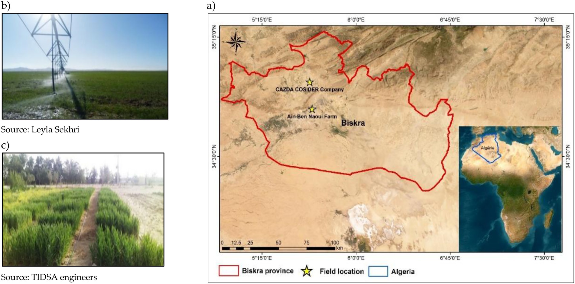
Figure 1. Location map (https://earthexplorer.usgs.gov/) of the study area and experimental field (a), Calibration (b), and Validation (c) process of AquaCrop for durum wheat.

Figure 2

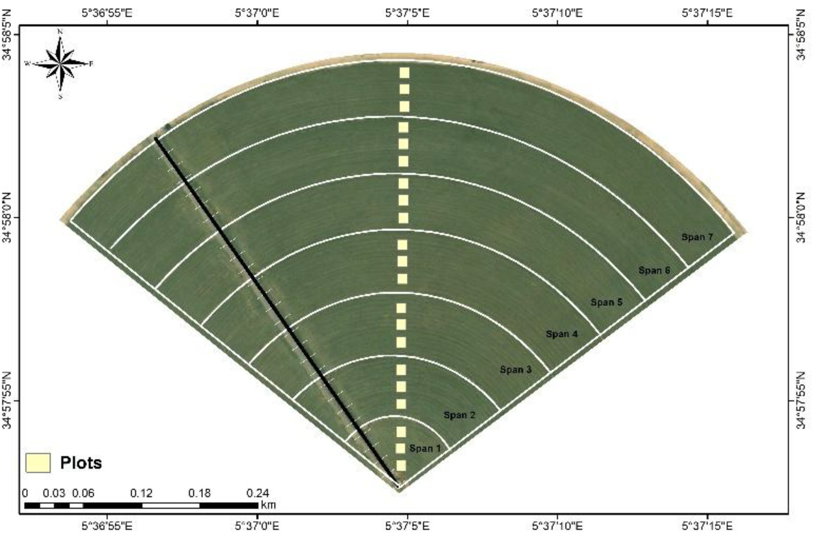
Figure 2. Quarter section of the center pivot showing the experimental design.

2.2 Field experiments

In the current study, a pivotal irrigation system of ANABIB type was used to provide irrigation water during the growing period, this system consisted of seven span towers, with a total length of 356 meters, irrigating a total area of 40 hectares. The experimental field used for model calibration was included in a quarter section of the center pivot, which covered 10 ha out of the total of 40 ha due to its large surface area, to ensure the validity of the results, it was crucial to consider the spatial heterogeneity of the soil, crop yield, canopy cover, and water distribution. Consequently, 21 experimental plots were arranged along the pivoting ramp, with 3 plots in each span, each plot size was 5.0 m × 10.0 m (50 m²) as illustrated in Figure 2, this experimental design was specifically implemented to minimize the impact of variability in water distribution on the accuracy of field measurements. All essential model input parameters and observed data necessary for the simulation were measured and calculated for each plot individually, the averaged values across these plots were then used. Unlike the traditional irrigation methods commonly practiced in the region, the center pivot system used in this study incorporates enhanced large-scale coverage. Although not yet widely adopted, this approach was selected to evaluate the model’s performance under optimized irrigation conditions, and to explore its potential applicability in modernizing irrigation practices in the area.

2.3 Crop management

In this study, all cultivation practices followed the approved agricultural protocol of the farm, which is designed to optimize wheat productivity and water use efficiency. Stubble cultivation was initiated on 11 August 2022; seedbed preparation involved deep plowing on 25 September 2022, followed by a second plowing on 29 October 2022. Wheat sowing took place on 22 November 2022 using a seeder at a rate of 160 kg ha⁻¹, and harvesting occurred on 20 May 2023. All cultivation operations were conducted in accordance with the farm’s protocol and under the supervision of its agricultural engineers. The protocol includes the following steps: stubble cultivation was initiated on 11 August 2022; the seedbed was prepared by deep plowing on 25 September 2022, followed by a second plowing on 29 October 2022. The wheat was sown on 22 November 2022 using a seeder at a rate of 160 kg ha⁻¹. Fertilization was applied as follows: 300 kg ha⁻¹ of Mono-Ammonium Phosphate (MAP) before sowing; 100 kg ha⁻¹ of urea (46% N) broadcasted at 60 days after sowing (DAS); followed by a second fertigation application of 50 kg ha⁻¹ at 120 DAS. Additionally, 2 liters per hectare of liquid potassium were applied via fertigation at 155 DAS. Weed and disease management included herbicide application at the beginning of February 2023, and preventive fungicide (Amistar Xtra) application at the end of February 2023 at a dose of 1 L ha⁻¹. For the validation site, each plot was planted at a density of 300 seeds per m², this site was carefully selected after confirming that the crop did not experience water stress or nutrient deficiency during the growing season. The seeding density was defined according to the local agricultural practices at each site. This site-specific approach ensures that the model is tested and validated under realistic and diverse planting conditions, enhancing both robustness and practical applicability.

2.4 Data collection

2.4.1 Soil data

At the calibration site, soil samples were collected from nine randomly selected locations within the experimental field to a maximum depth of 1.0 m. Sampling was conducted at fixed depth intervals of 20 cm before the beginning of the cropping season. Physical and chemical parameters such as texture, soil water content, electrical conductivity (EC) and bulk density were determined in the laboratory. Soil texture at different depths was classified using the soil textural triangle. Additionally, the hydraulic properties of the soils (wilting point, water content at saturation, saturation hydraulic conductivity) were estimated for both the calibration and validation sites using the soil hydraulic properties calculator based on predetermined soil particle size distribution (Saxton and Rawls, 2006). A curve number of 61 was employed as the default value for effective field management. The initial soil water content was assumed to be at the wilting point due to the arid conditions and absence of precipitation prior to sowing. The simulation period began in August to accurately represent field conditions at the start of the growing season. Table 1 summarizes the soil characteristics for both the calibration and validation locations used in this study.

Table 1

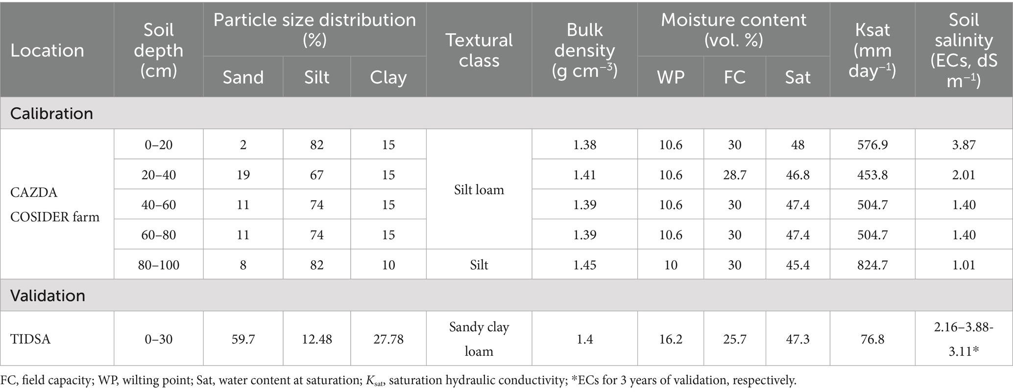
Table 1. Soil dataset used for calibration and validation of AquaCrop for the durum wheat crop.

The soil water contents (SWC in % vol.) were measured 5 times during the cropping seasons by the gravimetric method, on 20 December, 17 January, 15 March, 20 March and 11 April. at soil depths 20, 40, 60, 80 and 100 cm, then, soil samples were dried in an oven for 24 h at 105 °C. SWC was calculated by multiplying the gravimetric soil water content by the soil’s bulk density.

2.4.2 Crop data

Oued El-Bared is a durum wheat variety used in this study, that was monitored weekly to collect both model input parameters and observed field data; such as sowing date, the appearance of phenological stages; including days to reach the germination, maximum canopy cover, flowering, canopy senescence, and crop maturity, were observed and recorded throughout the growing season. The green canopy cover development was monitored every week; a measurement point was identified for each plot, and photographs were taken at noon above the plant cover with a digital camera. The images were analyzed using the Green Crop Tracker (Version 1.0) software, developed by Agriculture and Agri-Food Canada (Liu and Pattey, 2010) to determine the crop canopy cover rate (CC in %). Plant density was estimated by counting the number of plants within a 1 m² quadrat placed in each plot. The wheat was sampled 5 times from crop establishment to harvest on 15 March, 23 March, 12 April, 25 April and 14 May. For each sample; micro-plots of ¼ m² were selected in each plot, and the aboveground biomass was determined by drying the samples in an oven (at 70 °C) until a constant weight was obtained, to evaluate the temporal evolution of the wheat biomass. Finally, representative samples of 1 m² from the middle of each plot was harvested and dried in a safe location to determine the final grain yield and above-ground biomass (B in ton ha⁻¹). The harvest index (HI) was defined as the percentage ratio of wheat grain yield to final above-ground biomass. At the TIDSA validation site, field experiments were carried out over three consecutive cropping seasons: 2020/2021, 2021/2022, and 2022/2023, using the same durum wheat variety. The sowing dates were November 23, 2020, November 28, 2021, and November 23, 2022, respectively, while crop maturity was reached on May 4, 2021, May 11, 2022, and May 4, 2023.

2.4.3 Meteorological data

The meteorological data used in this study to calibrate and validate the model were collected from the Biskra meteorological station, the dataset included daily precipitation, relative humidity, temperatures (maximum and minimum), solar radiation, and wind speed. The annual mean CO₂ concentration data from the Mauna Loa Observatory in Hawaii, included as a default file in AquaCrop, was used in the model. To calculate the daily reference evapotranspiration (ETo) values; ETo calculator (version 3.2, September 2012) for Land and Water Division in FAO organization was used, based on Penman-Monteith method (Allen et al., 1998). Figure 3 presents the daily meteorological data, including maximum and minimum air temperatures, reference evapotranspiration (ETo), precipitation, wind speed, and relative humidity, from 1 August 2020 to 31 May 2023, used for model calibration and validation. The region exhibited significant seasonal temperature variations. Maximum temperatures (T_max) often exceed 40 °C during the summer months (June to August), with peaks reaching up to 48.7 °C. In contrast, the winter months (December to February) experienced cooler temperatures, with minimum temperatures (T_min) occasionally dropping below 10 °C (Figure 3a). The average daily maximum and minimum temperature during the wheat growing seasons were 19.2 ± 7.1 and 10.3 ± 6.8 °C, respectively. Precipitation was sparse and highly variable, with most precipitation concentrated between late autumn to late spring (Figure 3c). Total precipitation during the wheat growing seasons exhibited substantial interannual variability across the study period: 30.99 mm in 2020–2021, 45.72 mm in 2021–2022, and 54.10–58.42 mm in 2022–2023 and ET₀ during the seasons analyzed in this study was 728, 579.7, 622.6, 771 mm, respectively. The Lowest ET₀ consistently occurred in winter months (December–January), while the highest ET₀ was observed in spring (March–May), as represent in Figure 3c.

Figure 3

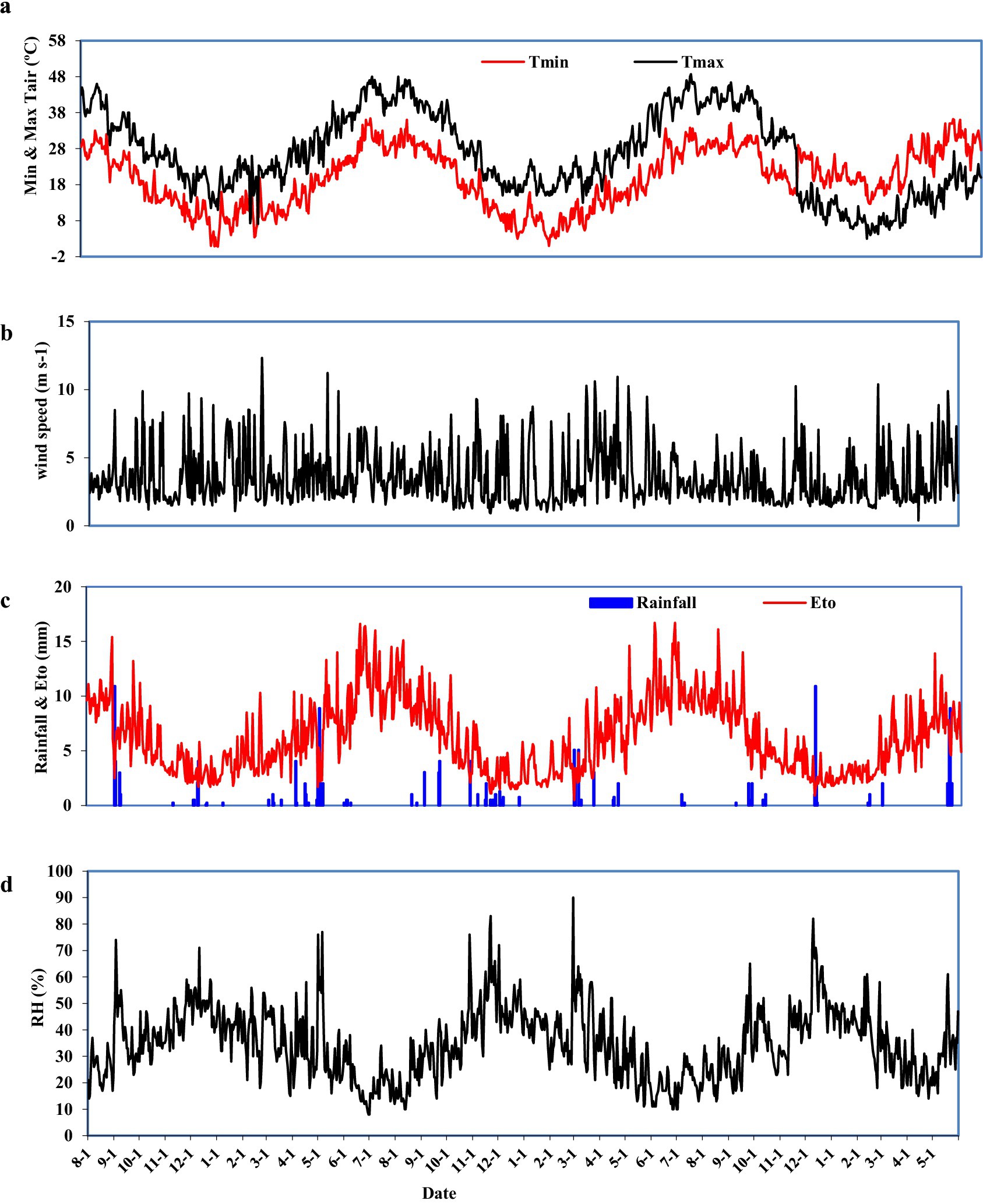
Figure 3. Daily weather data at the study area (from 1 august 2020 to 31 may 2023), (a) maximum (Tmax) and minimum (Tmin) air temperatures (°C), (b) wind speed (m s⁻¹), (c) rainfall and reference evapotranspiration (ET_o) (mm), (d) relative humidity.

2.5 Irrigation practices

Irrigation was conducted using 3 wells in CAZDA COSIDER farm. Water is pumped into a geomembrane basin with a capacity of 30,000 m³ according to the water consumption of the wheat. The irrigation applied in this study followed the irrigation practices implemented by the farm engineers at CAZDA COSIDER throughout the growing season. A total of 25 irrigations were applied during the season, the volume of water for each irrigation event was measured accurately using a water meter. Using the start dates of the pivoting ramp rotation and the rotation angles, the irrigation events in the experimental plots were identified. The irrigation volumes varied widely (from 10 to 120 mm per event) according to the growth stage of the crop and prevailing climatic conditions, with larger amounts during early establishment and reduced volumes during later growth stages. Each irrigation event was entered into the AquaCrop model with its specific date and applied amount, to ensure accurate field management and simulate soil water dynamics. Electrical conductivity (EC_iw) and pH of the irrigation water were measured in situ using a multi-parameter manual instrument HI98129 and HI98130 waterproof pH, EC/TDS and Temperature tester, water electrical conductivity (EC_iw) was 4.46 dS m⁻¹ and a pH of 7.95. For model validation at the TIDSA site, irrigation was supplied by drip systems over three seasons; in 2020/2021, 52 irrigation events were applied (EC_iw: 6.05 dS m⁻¹, pH: 7.73); in 2021/2022, 38 events were applied (EC_iw: 4.52 dS m⁻¹, pH: 7.53); and in 2022/2023, 42 irrigation events were applied (EC_iw: 6.18 dS m⁻¹, pH: 7.87). All irrigation data collected throughout three growing seasons directly entered into the model, a description of the irrigation water used to calibrate and validate the AquaCrop model is provided in the Table 2. The differences in the number and frequency of irrigation events between the calibration and validation sites are attributed to key factors including the irrigation systems and soil characteristics. The calibration site employed center pivot irrigation, which covered a larger area and required longer durations to complete each event, resulting in fewer but larger irrigation applications. In contrast, the validation site employed drip irrigation, which delivered smaller amounts of water more frequently. The site’s soil texture exhibits intermediate water-holding capacity and permeability, which, when combined with elevated evapotranspiration rates, requires more frequent irrigation to sustain optimal soil moisture levels for crop growth. These site-specific irrigation practices were incorporated into the simulation model to ensure accurate representation of soil water dynamics and crop response.

Table 2

Table 2. Irrigation depths (mm) for calibration and validation locations.

2.6 AquaCrop model description

The AquaCrop simulation model developed to predict the yield of herbaceous crops response to water (Steduto et al., 2012). The model’s detailed descriptions are presented by Hsiao et al., 2009, Raes et al. (2009), Steduto et al. (2009a), and Raes et al. (2018). In various studies, the model has been employed to simulate the growth responses of various crops to irrigation water and environmental conditions in several regions; wheat (Andarzian et al., 2011; Goosheh et al., 2018; Iqbal et al., 2014; Jin et al., 2018; Kumar et al., 2014), maize (Greaves and Wang, 2016; Paredes et al., 2014b), sugarbeet (Garcia-Vila et al., 2019), grain sorghum (Araya et al., 2016). AquaCrop is designed to be widely applicable across different climates and soil conditions, minimizing the need for extensive local calibration. To achieve this, the model constructed with two main groups of parameters: conservative parameters (Raes et al., 2009; Steduto et al., 2009a), which remain constant across different crop cultivar, location and time (Steduto et al., 2012). The second group non-conservative parameters, obtained through field measurements, as detailed in Tables 3, 4. In the calibration and validation phases, it is necessary to compare the simulated results with the field measurements. During the calibration of the model; the values of the non-conservative crop parameters were employed to minimize the differences between the predicted and observed results (Steduto et al., 2012). The model simulates crop growth on a daily time step and requires a reduced set of input parameters for its operation, including weather data, crop characteristics, soil properties, and management practices (such as irrigation and field operations) specific to the site. In this study, AquaCrop (version 7.1, graphical user interface [GUI] edition, FAO, Rome, Italy) was used for simulation. AquaCrop simulates crop yield in response to water availability through five interconnected phases that integrate soil, crop, and atmospheric conditions. The process begins by modeling the development of the crop canopy cover (CC, %), which is calculated from the maximum canopy cover (CC_x, %) and a canopy expansion rate coefficient (K_c) over time (Equation 1). Next, crop transpiration (Tr, mm) is estimated as a function of an adjusted canopy cover (CC*, %), a maximum crop transpiration coefficient (K_{CTr, x}), and the potential crop evapotranspiration (ET_o, mm) and water stress (Equation 2). Biomass production (B, t/ha) is then calculated by multiplying a water productivity factor (WP, g/m²) by the cumulative transpiration (ΣT_r, mm) over the growing season (Equation 3). The final crop yield (Y, t/ha) is derived from the produced biomass and a harvest index (HI) (Equation 4). Finally, the overall water productivity (WP_ET, kg/m³) is computed as the ratio of yield to the total evapotranspiration water loss (ET, mm) as represent in Equation 5 (Iqbal et al., 2014; Raes et al., 2009; Steduto et al., 2009b; Wang et al., 2022; Zhai et al., 2022):

$\begin{array}{ll}\mathit{CC}={\mathit{CC}}_x(1-e^{-K_c(t-\mathit{\text{to}})})& (1)\end{array}$

$\begin{array}{ll}{T}_r=(C{C}^{\ast }\times K_{C{T}_r,x}){\mathit{ET}}_o& (2)\end{array}$

$\begin{array}{ll}B=\mathit{WP}\times \sum T_r& (3)\end{array}$

$\begin{array}{ll}Y=\mathit{HI}\times B& (4)\end{array}$

$\begin{array}{ll}W{P}_{\mathit{ET}}=\frac{Y}{\mathit{ET}}& (5)\end{array}$

Table 3

Table 3. The conservative input parameters used in the study to calibrate AquaCrop, and values used in previous studies for wheat crop.

Table 4

Table 4. Non-conservative crop parameters used for calibration of the model.

2.7 Sensitivity analysis

Sensitivity analysis (SA) is a useful tool for identifying the parameters that exert the most significant influence on model outputs (Cao and Petzold, 2006). Thereby guiding the calibration of the model and enhancing the accuracy of simulations. The SA identifies the parameters that most strongly influence model outputs, highlighting those that require the most precise field measurements and careful calibration (Mohammadi et al., 2016). To assess the robustness of the AquaCrop model for durum wheat and to determine the quality requirements of its input data, a sensitivity analysis was conducted prior to model calibration by varying key crop, soil, and climatic parameters. An input variation range of ± 20% was applied to each parameter during the sensitivity analysis. The analysis focused on a selected set of crop, soil, and irrigation management parameters (Table 5), with simulations performed with the corresponding data of the calibration field conditions. Simulated wheat grain yield was used as the primary output for evaluating sensitivity. This approach provided a systematic assessment of how variations in input parameters affect model performance and identified the most critical parameters requiring careful consideration for reliable model application. After changing the input parameters, the model outputs were evaluated against the baseline outputs by calculating the sensitivity coefficient (S_c), as defined by Geerts et al. (2009), as represent in Equation 6.

$\begin{array}{ll}{S}_C=\mid \frac{P_a-P_b}{P_b}\mid \times 100& (6)\end{array}$

where; P_a is the model output after changing the input value and P_b is the output before the change. Sensitivity classes were defined as high, moderate, or low when the model response to input changes was greater than 15%, between 15 and 2%, or less than 2%, respectively (Geerts et al., 2009).

Table 5

Table 5. Crop parameters evaluated in the sensitivity analysis of AquaCrop, for durum wheat yield under ±20% variation of input parameter.

2.8 Calibration and validation procedures

In this study, AquaCrop was calibrated and validated, for durum wheat, using field data from agricultural sites affected by salinity. Validation under real field conditions provides practical insights into model performance and supports its adoption in actual agricultural production, complementing results obtained from controlled experiments. The AquaCrop model was parameterized for the experimental field within a central pivot irrigation system, and the calibration process was performed by running the model with the specific input data on weather conditions, soil characteristics, field managements practice, and crop parameters. It was selected because it provided a comprehensive and well-documented dataset, including regular measurements of CC, above-ground biomass, SWC, and final grain yield. Regarding model validation, data from a different site (TIDSA) were used; the validation process involved comparing the simulated and observed values of final gains yield only, using a combined dataset, which included: (1) Experimental data from the CAZDA COSIDER farm during the 2022–2023 cropping season. (2) Data from experiments conducted by TIDSA engineers during 2020–2021, 2021–2022 and 2022–2023 cropping seasons. It should be noted that the validation was restricted to grain yield due to the unavailability of measured data on SWC and CC at the validation site; however, grain yield is a key indicator of overall crop performance and provides meaningful insights into the model’s predictive capability under the studied conditions. Future studies should aim to include additional datasets to allow a more comprehensive validation of model outputs. The methodological steps followed in this study are summarized in Figure 4.

Figure 4

Figure 4. Flowchart summarizing the methodological steps in this study for the calibration, simulation, evaluation, and validation of AquaCrop 7.1 model for durum wheat.

The conservative parameters in AquaCrop should initially be retained at their default values and may be adjusted when strong supporting data is available if there is a clear need, because these values were determined using modern high-yielding cultivars grown under ideal water and soil conditions, adjusting these parameters may be justified when applying the model to lower-yielding or rustic crop cultivars (Steduto et al., 2012). Boulange et al. (2025) demonstrated that in the published literature, there is a widespread tendency to calibrate both conservative and non-conservative parameters of the AquaCrop model for cotton crop, even in studies conducted under similar environmental and climatic conditions, this practice results in significant variation of calibrated parameter values, which raises concerns about over-calibration and diminishes the model’s transferability across different sites or conditions. The AquaCrop handbook emphasizes that the model relies on a group of conservative parameters, described as “generally applicable and not requiring local calibration” or “parameters that should remain largely unchanged across different growing conditions and water management regimes (Raes, 2023; Raes et al., 2023). They are also generally considered invariant across cultivars unless demonstrated otherwise; examples include the stress thresholds and the normalized water productivity (WP*) (Raes, 2023).

Previous calibration and validation efforts in AquaCrop produced favorable results for wheat crop, the cases cited in Table 3 illustrate that some studies maintain conservative parameters at their default values, will others show variability in the adjustments of these parameters such as WP*, base temperature, and stress thresholds. In the current study, conservative parameters were not calibrated, and maintained at their default values, as specified in the AquaCrop wheat crop file (Table 3); because the Oued El-Bared cultivar is a modern, high-yielding variety, it is unnecessary to adjust these conservative parameters.

Afterwards, based on the averaged measurements obtained from the CAZDA COSIDER field experiment, the available monitored data were assigned to the corresponding non-conservative parameters (Table 4). Parameters that could not be measured in the field were either calibrated based on the available data or estimated internally by the model. The model estimated CCo based on the measured planting density and the default value of canopy cover per seedling at 90% emergence. Canopy growth coefficient (CGC) and the canopy decline coefficient (CDC) were not directly quantified through field measurements. Instead, by entering key phenological dates for the studied crop cultivar (dates of emergence, maximum canopy cover, senescence and maturity), the model automatically estimated their values. Iterative model simulations were conducted to finely adjust the rooting depth, aiming to achieve the best agreement between simulated and observed values of canopy cover, above-ground biomass, final above-ground biomass and soil water content at different growth stages. In this study, most of the non-conservative parameters were obtained directly from field measurements. As a result, only minimal manual adjustments were applied, and a trial-and-error calibration approach was not required extensively.

After the calibration process, model validation was performed while all other calibrated parameters were considered as constants during this stage; the validation process involved assessing the agreement between simulated and observed final grain yield values, to ensure that the model accurately represented all crop growth phases, including the final yield. The model was also run with the default wheat crop file in the Growing Degree Days (GDD) mode, the process was carried out for both locations to evaluate the model’s performance in predicting key outputs, including final grain yield, above-ground biomass, soil water content (SWC) and final above-ground biomass.

2.9 Model evaluation

Green canopy cover, above-ground biomass development, soil water content, final grain yield and final above-ground biomass were considered for model evaluation, model outputs were assessed against field measurements using statistical indices, which included:

1. The root means square error (RMSE), presented by Equation 7, was applied to evaluate the model performance, when RMSE value close to zero indicates better model performance, 0 indicating perfect and indicating poor model performance.

$\begin{array}{ll}\mathit{\text{RMSE}}=\sqrt{\frac{\sum _{i=1}^n{(S_i-M_i)}^2}{n}}& (7)\end{array}$

2. Normalized root-mean square error (NRMSE), presented by Equation 8:

$\begin{array}{ll}\mathit{\text{NRMSE}}=\frac{\sum _{i=1}^n{(S_i-M_i)}^2}{n}\times \frac{100}{M}& (8)\end{array}$

The simulation is considered excellent with a NRMSE < 10%, good if it is between 10 and 20%, fair if it is between 20 and 30%, and poor if the NRMSE >30% (Jamieson et al., 1991).

3. Nash-Sutcliffe model efficiency coefficient (EF), presented by Equation 9 a normalized statistic determines the relative magnitude of the residual variance compared to the measured data variance (Nash and Sutcliffe, 1970).

$\begin{array}{ll}\mathit{EF}=1-\frac{\sum _{i=1}^n{(S_i-M_i)}^2}{\sum _{i=1}^n{(M_i-\overline{M})}^2}& (9)\end{array}$

where; EF ranges between -$\infty$ $<\mathit{EF}\le$ 1; EF = 1 being the optimal value, 0 $<\mathit{EF}<$ 1 acceptable levels of performance, negative values indicate that the mean measured value is a better predictor than the simulated value (unacceptable performance) (Moriasi et al., 2007).

4. Willmott’s index of agreement (d), was developed by Willmott (1981), which is a standardized measure of the degree of model prediction error (Equation 10); it ranges between 0 and 1; d = 1 indicates a perfect agreement between measured and simulated values, and d = 0 indicates no agreement (Willmott, 1981).

$\begin{array}{ll}d=1-\frac{\sum _{i=1}^n{(S_i-M_i)}^2}{\sum _{i=1}^n(\mid \mathit{Si}-\stackrel{¯\mid }{M}+\mid M_i-\stackrel{¯\mid }{M})2}& (10)\end{array}$

where; − $\infty$ $<d\le$ 1; better agreement between simulated and measured values achieved when values of d close to 1.

5. Pearson Correlation Coefficient (R), ranges from 0 to 1, with values close to 1 indicating good agreement (Equation 11).

$\begin{array}{ll}R=\frac{\sum _{i=1}^n(M_i-\overline{M})(S_i-\overline{S})}{\sqrt{\sum _{i=1}^n{(M_i-\overline{M})}^2\sum _{i=1}^n{(S_i-\overline{S})}^2}}& (11)\end{array}$

where; M_i and S_i (i = 1, 2,…, n) indicate measured and simulated values, respectively, and $\overline{M}$: the mean of measured values and n is the total number of observations in all statistical indices.

3 Results and discussion

3.1 Sensitivity analysis (SA)

Table 5 presents the results of the SA conducted using a ±20% variation in each individual parameter while keeping all other parameters constant. The purpose of the SA is to identify the differences in the way AquaCrop responds to changes in specific inputs for simulating grain yield. The S_c values and their signs indicate both the magnitude and direction of change in grain yield relative to the baseline simulation.

The results of the SA for simulated final grain yield indicated that AquaCrop was highly sensitive to changes in WP* and HI₀, which exhibited the largest absolute sensitivity coefficients. Soil and irrigation water salinity collectively impose osmotic and ionic stresses that limit the plant’s ability to take up water and disrupt physiological processes essential for biomass production and partitioning. This stress reduces WP* and negatively affects the allocation of biomass to the grain (lowering HI₀). Under arid conditions such as those in Biskra, this combined salinity stress leads to significant declines in both WP* and HI₀.

Canopy development parameters such us CGC, time from sowing to maximum canopy cover, CCx, and CCo showed moderate sensitivity, suggesting that early-season canopy structure plays an important role in determining final yield. In particular, when these parameters were decreased, slower canopy development or delayed attainment of maximum cover markedly reduced grain yield. The canopy decline coefficient (CDC) also demonstrated consistent moderate sensitivity, reflecting the importance of maintaining canopy cover during the late growth stages to optimize yield formation. Similarly, the crop transpiration coefficient (KcTr) and maximum rooting depth had moderate influence, highlighting the link between water uptake dynamics and yield outcomes.

In contrast, the model showed low sensitivity to changes in phenological parameters such as time to flowering, flowering duration, and emergence, as well as to stress-related parameters including EC thresholds, canopy expansion, and early canopy senescence. Under the environmental conditions of this study, these factors had minimal impact on simulated yield.

The sensitivity analysis of soil parameters in AquaCrop revealed that FC exhibited moderate to high sensitivity, indicating that variations in FC substantially affect model output and should be carefully parameterized. WP showed moderate sensitivity, suggesting a secondary impact on simulated yield. Sat, Ksat, and ECs displayed low sensitivity, so variations in these parameters have a limited influence on model predictions. These findings highlight that accurate determination of FC is particularly critical for robust model performance.

The SA of irrigation management parameters in AquaCrop indicated that the amount of irrigation exhibited a wide range of sensitivity, from low to high, which reflects its variable influence on model outputs depending. Notably, the model showed high sensitivity to reductions in irrigation amount, which highlights the significant effect of water deficit on yield simulation. Conversely, irrigation water salinity (Ec_iw) displayed low sensitivity, suggesting that reasonable variations in water salinity have a limited effect on model predictions under the studied conditions.

SA itself does not improve the accuracy of field measurements. However, in this study, it provided critical insights into the relative influence of key parameters on model outputs. WP* and HIo were identified as the most influential parameters affecting these outputs. This finding informed targeted adjustments of these parameters within physiologically realistic ranges during the calibration process. Sensitivity analysis was therefore valuable not only for prioritizing parameters but also for optimizing the calibration strategy, resulting in reliable and accurate simulation outcomes under local conditions.

According to Geerts et al. (2009), a lack of sensitivity to certain parameters indicates possible over-parameterization of the model, whereas high sensitivity to others reflects a strong dependence of specific calculation processes on a limited set of parameters.

3.2 Model calibration

As stated in the previous section, the AquaCrop model was calibrated for durum wheat using experimental data of the CAZDA COSIDER farm, from the period: November 22, 2022, to May 20, 2023, The model was used with the specific conditions of the pivot irrigation system, which is crucial for enhancing water management strategies and achieving optimal crop yields, Validation was performed using the TIDSA dataset. The model’s performance and robustness were assessed by comparing simulated and observed values of green canopy cover, above-ground biomass, soil water content, final above-ground biomass, and final grain yield. Besides the differences in irrigation methods, the two sites varied in key agronomic and environmental factors influencing irrigation performance. The calibration site, which used center pivot irrigation, had a different soil texture and water retention capacity compared to the validation site, where drip irrigation was employed. Additionally, planting densities varied, with the validation site typically using denser planting. The frequency and volume of water applications (number of irrigations) also differed between sites, shaped by the irrigation system capabilities and crop water requirements. The model was calibrated and validated using modern irrigation techniques to encourage the adoption of advanced irrigation technologies, particularly under the current conditions where surface irrigation remains widely used despite growing water scarcity in Biskra as well as across Algeria. According to recent statistics, approximately 43.54% of the total irrigated areas in Biskra still rely on traditional surface irrigation methods, whereas water-saving techniques like drip irrigation cover about 49.26%, while sprinkler and center pivot irrigation occupy smaller proportions, approximately 5.66 and 1.52%, respectively (DSA, 2022). This highlights the urgent need to promote efficient irrigation systems to better conserve scarce water resources and support sustainable agricultural development in the region. Fonteyne et al. (2021) reported that water use in the barley-maize production system can be reduced by 20–40% through the implementation of conservation agriculture, drip irrigation, or a combination of both. Similarly, Tang et al. (2025) demonstrated that combining wide–narrow row spacing with moderate drip irrigation significantly maintained yield and improved water-use efficiency in winter wheat production in arid regions. Ahmed et al. (2017) showed that high-efficiency irrigation systems, particularly center pivot irrigation, significantly enhance water and crop productivity in seed multiplication, reducing water losses by about 10 to 20%.

3.2.1 Canopy cover (CC)

Figure 5 displays a comparison between the observed and simulated CC values over different days after sowing using both the calibrated and default crop parameters. A strong linear correlation was found between the observed and simulated values for both cases, with R² values of 0.98 for the calibrated simulation and 0.89 for the default simulation, the statistical evaluation of this parameter is presented in Table 6.

Figure 5

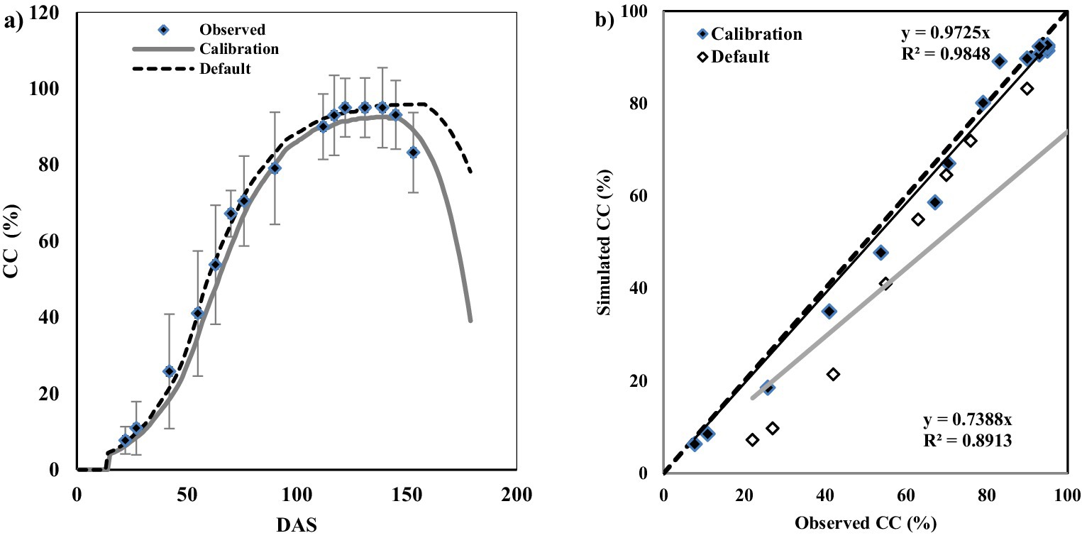
Figure 5. Observed and simulated values of canopy cover (CC) on different days after sowing (DAS) during model calibration: (a) temporal comparison of observed and simulated CC throughout the growing season; (b) relationship between simulated and observed CC, with diagonal lines represent 1:1 line.

Table 6

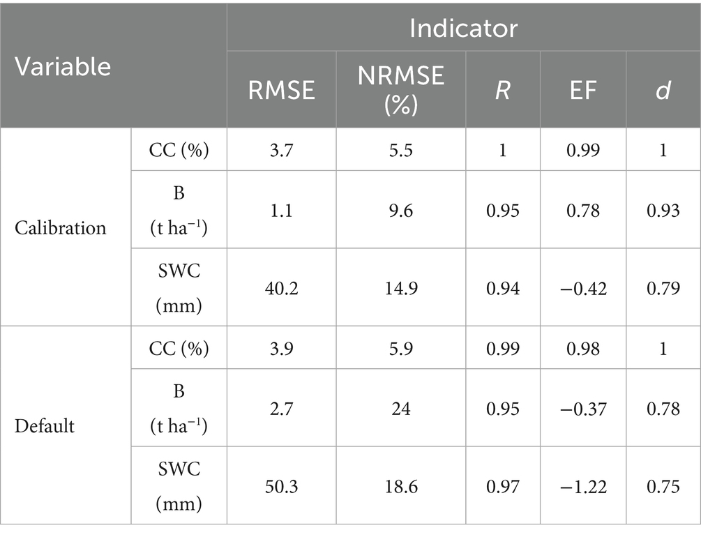
Table 6. Statistical performance indicators for observed and simulated canopy cover, Above-ground biomass, and soil water content for both calibrated and default model settings.

Simulation results using default parameters indicated that the model demonstrated excellent performance in simulating CC, with high statistical indicators (R = 0.99, RMSE = 3.9, NRMSE = 5.9%, EF = 0.99 and d = 1) (Table 6). However, slight differences can be noted; the default parameterization led to minor deviations and, overall, produced a marginally higher error compared to the calibrated scenario.

The model showed better prediction of CC when calibrated parameters were used, and demonstrated excellent performance in simulating CC development, with a very strong agreement between observed and simulated CC values, the statistical indicators confirm that model calibration improved the accuracy of canopy cover simulations, as reflected by lower values of RMSE = 3.7%, NRMSE = 5.5%, and a high model efficiency (EF = 0.99). The (d) values obtained indicate perfect agreement between the simulated and measured data (d = 1). Furthermore, the elevated R values suggested a perfect linear correlation between simulated and measured CC (R = 1). The model slightly underestimated CC during the early and mid-growth stages, specifically from 42 to 70 DAS and from 122 to 139 DAS (Figure 5). However, this underestimation, particularly in the later days of the season, coincided with reduced simulated available soil water (as shown in Figure 6), which is primarily attributed to the model’s increased sensitivity to water stress during this period. Hsiao et al. (2009), reported that there was an overestimation of the inhibitory effect of a slight water deficit on the growth of the CC in maize. Sandhu and Irmak, 2019, reported that sampling and measurement errors, the influence of extreme temperatures and aridity could be caused differences in CC. Similar results observed by Rinaldi et al. (2011) and Heng et al. (2009) as underestimation in the simulation. Overall, only minor differences were observed, and the model provided a reliable estimation throughout the growing season.

Figure 6

Figure 6. Observed and simulated values of soil water content (SWC) in the top 1 m on different days after sowing (DAS) during model calibration: (a) temporal comparison of observed and simulated SWC throughout the growing season; (b) relationship between simulated and observed SWC, with diagonal lines represent 1:1 line.

3.2.2 Soil water content

In this study, the model was applied in a large area under center pivot irrigation conditions. To enhance the precision of the soil water content (SWC) simulation, spatial heterogeneity of soil properties, irrigation amounts, and the occurrence of irrigation events were taken into-consideration. For Simulation results using calibrated parameters, SWC approached or exceeded the field capacity line during the early vegetative growth stage, which caused percolation; during this period the model simulated well the SWC. In contrast, in the residual cropping season, SWC remained between the field capacity and wilting point lines, the linear correlation between observed and simulated SWC was strong (R² = 0.77), the model trended to underestimate the SWC in this period. For comparison, simulations based on the model’s default crop parameters generally resulted in higher SWC values throughout the season, clearly visible as an overestimation trend in (Figure 6). When the default parameters were used, the model’s ability to simulate SWC declined, as reflected by higher error indices (RMSE = 50.3 mm, NRMSE = 18.6%), slightly improved correlation (R = 0.97), but lower index of agreement (d = 0.75) and a more negative EF (EF = −1.22). This suggests that while the default parameters allowed the model to capture the general fluctuations in SWC, its performance was poorer compared to the calibrated scenario. Paredes et al. (2014b) reported similar findings and emphasized the importance of parameterizing the AquaCrop model using accurate and continuous SWC observations throughout the crop growing season. They highlighted that thorough calibration based on detailed field measurements significantly enhances the model’s reliability in simulating SWC and crop performance.

The results of the SWC using calibrated parameters show that the model performed well for simulating the SWC in the root zone (0–100 cm), as shown by the statistical indices: RMSE = 40.2 mm, NRMSE = 14.9%, R = 0.94 and d = 0.79 indicating a good agreement between measured and simulated values. Despite the negative value of the Nash–Sutcliffe Efficiency (EF = −0.42), other model performance indicators showed good values, indicating that the model was able to capture the temporal patterns and general trends of soil water content dynamics. However, the negative EF indicates that the observed mean of soil water content (SWC) would provide a better estimate than the model simulations. This suggests that, although the model was able to capture the general temporal trends of SWC, it exhibited significant differences in simulating the actual observed values, particularly during the late season under combined water deficit and salinity stress (Table 6). A positive Nash–Sutcliffe Efficiency (EF) is considered the minimum criterion for reliable soil water content simulation in crop models (Yang et al., 2014). Terán-Chaves et al. (2022) has been documented similar discrepancy in simulating SWC using AquaCrop, characterized by negative EF values, and reported that the observed mean serves as a better predictor than the model simulations. The negative EF value observed reveals the model’s limitations in accurately simulating observed SWC, particularly under the combined influence of salinity and drought stresses during the late growing season. The underestimation of SWC most likely resulted from an inaccurate estimation of evapotranspiration and the model’s inability to fully capture the combined effects of salinity and water stress on plant water uptake. These stresses reduce root water absorption efficiency and disrupt the soil–plant-water balance, leading to lower simulated SWC. Additionally, simplified parameterization under stress conditions may have contributed to an overestimation of water loss. This interpretation aligns with numerous studies worldwide, which report that the interaction between salinity and limited irrigation reduces water availability to plants and challenges the model’s capacity to accurately represent these complex stress conditions. Zhai et al. (2022) reported that the AquaCrop model demonstrated good performance in simulating SWC across various irrigation levels and water salinity conditions for winter wheat, model performance indicators (R², RMSE, NRMSE) were 0.87–0.95, 1.22–2.59%, and 8.09–12.95% during calibration, and 0.88–0.96, 1.52–2.75%, and 10.32–18.12% during validation, respectively, however, simulation accuracy declined under deficit irrigation with saline water. Mohammadi et al. (2016) calibrated and validated the AquaCrop model for wheat to simulate SWC under combined salinity and water stress conditions in an arid region, their results showed good agreement between simulated and observed soil moisture, with an average normalized root mean square error (NRMSE) of 11.8%, an index of agreement (d) of 0.79, and a coefficient of determination (R²) of 0.61, the model exhibited a tendency to systematically underestimate SWC. In contrast, Mkhabela and Bullock (2012) reported the overestimation of SWC for wheat, with corresponding model performance statistics of RMSE = 49.4 mm, R² = 0.9, and d = 0.99 Their evaluation metrics showed strong agreement between observed and simulated SWC values, with R² ranging from 0.87 to 0.96 and normalized root mean square errors (NRMSE) between 8.09 and 18.12% during both calibration and validation phases. However, they noted that simulation accuracy decreased under deficit irrigation combined with saline water. The accuracy in simulating SWC through the AquaCrop model is affirmed by results in other research for wheat (Andarzian et al., 2011; Benabdelouahab et al., 2016) which similarly reported a tendency to overestimate SWC.

Additionally, several studies have reported limitations in AquaCrop’s ability to accurately simulate soil water content, attributing underestimation or overestimation errors to various factors. Paredes et al. (2014b) found that AquaCrop shows a tendency to underestimate evaporation and overestimate transpiration, leading to a bias in SWC simulations. Farahani et al. (2009) found that errors in simulating SWC were non-uniformly distributed across the soil profile, with a tendency to overestimate in the surface layer and underestimate in deeper soil layers. Sandhu and Irmak (2019) reported that the inaccurate estimates of SWC could result from imprecise estimations of transpiration and evaporation, which relate to the utilization of inadequate or less accurate coefficients for transpiration and evaporation.

To improve model performance, future studies should refine the calibration of stress response parameters. Additionally, measuring SWC at multiple depths and at shorter intervals would provide a more detailed understanding of soil moisture dynamics and enable more robust model validation.

3.2.3 Above-ground biomass

Figure 7 illustrates the comparison between observed and simulated Above-ground biomass (B) values for durum wheat, using both calibrated and default crop parameters. When the default parameterization was applied, model performance declined noticeably, errors increased (RMSE = 2.7 t ha⁻¹, NRMSE = 24%) and a lower index of agreement (d = 0.78), and model efficiency became negative (EF = −0.37) (Table 6). This indicates that, although the default settings allowed the model to capture general B development trends, they led to larger deviations between observed and simulated values, especially during critical growth stages. The lower model efficiency and greater error metrics further underline the value of site-specific calibration for improving the accuracy of biomass simulation.

Figure 7

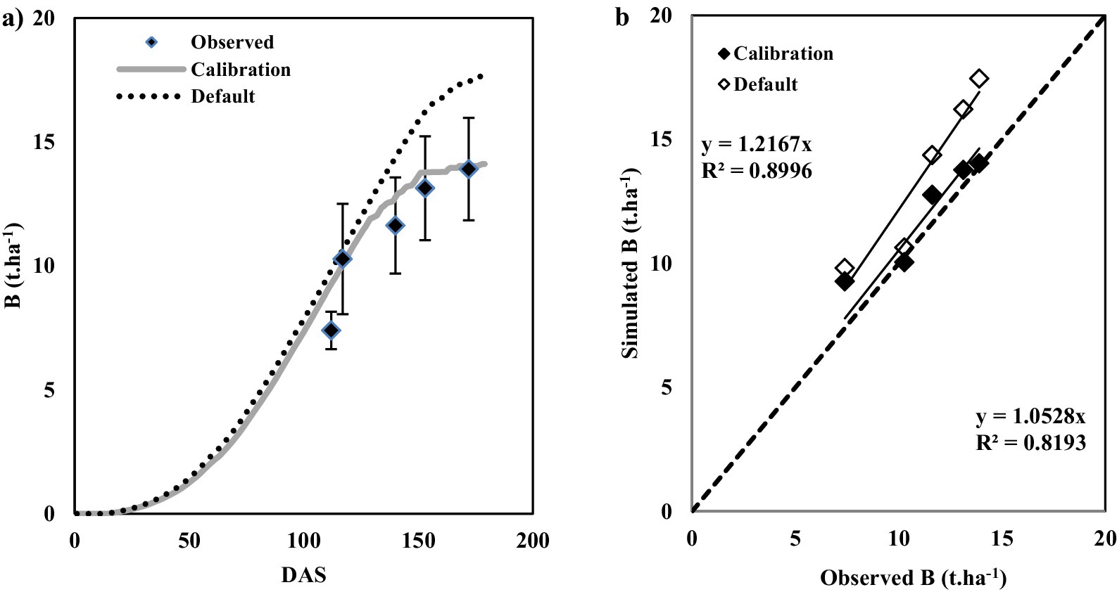
Figure 7. Observed and simulated values of above-ground biomass (B) on different days after sowing (DAS) during model calibration: (a) Temporal comparison of observed and simulated B throughout the growing season; (b) Relationship between simulated and observed B, with diagonal lines represent 1:1 line.

When using calibrated parameters, the linear correlation between observed and simulated values was strong (R² = 0.81), the model slightly overestimates B accumulation at 112, 140, and 148 DAS. Generally, AquaCrop performed very well in simulating the accumulation of (B) throughout the growing season, as shown by the model performance indicators; a root means square error (RMSE) of 1.1 t ha⁻¹, and a normalized RMSE (NRMSE) of 9.6% indicate a high level of model accuracy. A strong positive relationship was found between observed and simulated B (R = 0.95). Moreover, the model’s good performance is supported by the high value of EF, and an index of agreement (d = 0.93), which is close to 1, indicates a strong agreement between simulated and observed values (Table 5).

The predicted final above-ground biomass through the AquaCrop model was 14.1 t ha⁻¹, while the observed value was 14.35 t ha⁻¹, resulting in a very slight underestimation of 0.25 t ha⁻¹. This minor difference indicates that the model provides a close approximation of biomass accumulation under the studied conditions. Similar slight underestimation for wheat have been reported by Salemi et al. (2011) in arid region and Benabdelouahab et al. (2016) in semi arid region, Araya et al. (2010) for barley, and maize Hsiao et al. (2009). Contrasting results as an overestimation was noted by Andarzian et al. (2011) using the model for wheat. These variations observed across different crops and environments can be attributed to differences in cultivar characteristics, soil and climatic conditions, management practices and the specific methodologies employed for model calibration.

A slight overestimation of biomass accumulation occurred during intermediate growth stages, whereas a modest underestimation of the final above-ground biomass (0.25 t ha⁻¹) was noted at maturity. The observed decrease in SWC during the final growth stages (Figure 5) contributed to the decline in the final above-ground biomass compared to field observations. It becomes clear that the model overestimated the degree of water stress experienced by the crop at the end of the season. This outcome indicates that the model may be overly sensitive to reductions in soil moisture under these conditions, resulting in a reduction in predicted final above-ground biomass at maturity. Additionally, uncertainty arising from measurement errors in biomass sampling may also contribute to the observed differences between simulated and measured values; small differences likely reflect a combination of model sensitivity and unavoidable measurement errors, rather than being solely attributable to limitations in model performance.

In brief, the model accurately predicted the final above-ground biomass of durum wheat under saline environment and arid conditions of Biskra region.

3.3 Validation of the model

The validation process seeks to assess the model’s accuracy through comparisons of experimental data with output results (Thacker et al., 2004). In the current study, the model was validated using the same sets of conservative parameters values and statistical indices as those applied during the calibration phase. It was conducted using the method that was previously explained, In addition, model simulations were also performed using the default crop parameters provided by AquaCrop. Details of the data used for the validation were presented in the previous section. The model validation results of observed and simulated grain yields (t ha⁻¹) for durum wheat are presented in Table 7.

Table 7

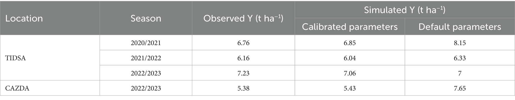
Table 7. Observed and simulated grain yields (Y) (t ha⁻¹) of durum wheat for both sites: model validation results.

Figure 8 presents the relationship between simulated and observed final grain yield under both calibrated and default model parameter sets. The regression line for the calibrated simulation is closer to the 1:1 line compared to that obtained with default parameters, indicating improved model performance after calibration.

Figure 8

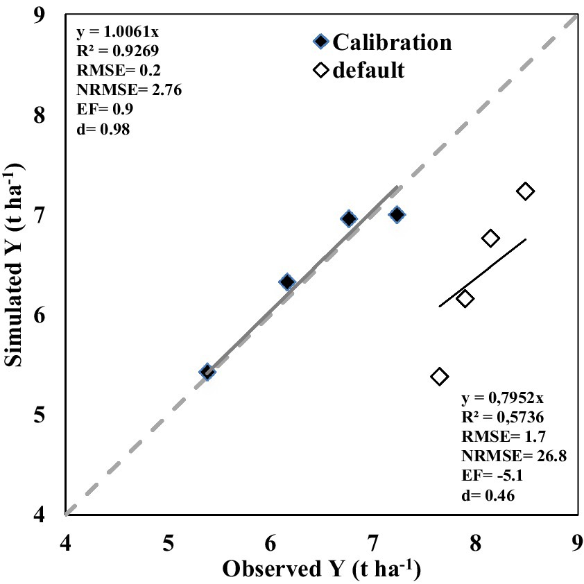
Figure 8. Relationship between observed and simulated durum wheat yield (t ha⁻¹) for both sites combined for the model validation.

Model simulations with default parameters showed that AquaCrop was inadequate in predicting final grain yield, as indicated by high errors and low efficiency (RMSE = 1.7 t ha-1, NRMSE = 26.8%, EF = −5.1, and d = 0.46) (Figure 8). The default parameters in AquaCrop often lead to an overestimation of crop yields because they are based on generalized assumptions about plant transpiration. These parameters usually depict optimal or average growing conditions and do not fully capture field-specific constraints such as water deficits, soil and irrigation water salinity, or nutrient limitations, which can directly reduce crop growth and yield. This highlights the necessity of using appropriately calibrated crop parameters to achieve reliable yield predictions.

In contrast, when calibrated parameters were applied, AquaCrop model predictions of grain yield showed excellent agreement with measured data for both sites and years. The pooled dataset revealed a low RMSE of 0.2 t ha⁻¹, NRMSE of 2.76%, high model efficiency (EF = 0.9), and index of agreement (d = 0.98). Additionally, there is a high correlation between the simulated and observed values, with a determination coefficient (R²) of 0.92. The slope is very close to 1, this demonstrates that the model’s predictions are unbiased, with no clear tendency for over- or under-prediction. Notably, all simulated yield values deviated from the observed values by less than 5%, this indicates a high level of model accuracy and no substantial bias in the predictions. Similarly, to assess the model’s robustness in simulating sugar beet yield in Spain, Garcia-Vila et al. (2019) used various factors including different locations, varieties, sowing dates, irrigation management and years to validate the model, and reported that the simulated yields showed a very good agreement with measured yields, with R² value 0.908 =, a slope = 0.945, RMSE = 1.17 t ha⁻¹, d = 0.998, without any clear trend for over-prediction or under-prediction. El Mokh et al. (2022) reported that the AquaCrop model is effective in simulating barley yield under saline and arid conditions in Tunisia, as evidenced by low RMSE values ranging from 0.36 to 1.6 t ha-1 and relatively high coefficients of determination between 0.77 and 0.81. Araya et al. (2010) used the model to simulate barley grain yield and reported an R² > 0.80 and the RMSE values range from 0.07 to 0.27 t ha⁻¹.

Mkhabela and Bullock (2012) used the model to simulate soft wheat grain yield and obtained over-prediction by only 3%, and the difference between the observed and simulated grain yield was 0.118 t ha⁻¹. Andarzian et al. (2011) and Benabdelouahab et al. (2016) reported that AquaCrop over-predicted grain yield for wheat (Triticum aestivum L.) and durum wheat, respectively. Salemi et al. (2011) reported that the model simulated very well winter wheat grain yield, with a slight under-prediction of 1.35%. These findings confirm the high predictive capacity of the AquaCrop model for durum wheat yield under the agro-climatic conditions of Biskra.

4 Conclusion

The calibration and validation of the AquaCrop model for durum wheat under the arid and saline conditions of Biskra, Algeria, demonstrated its strong capability in simulating key crop parameters, including canopy cover, above-ground biomass, soil water content, and final grain yield. In this study, the accurate calibration of canopy cover curve parameters, based on field-measured data, substantially improved the model’s performance. This enhancement is explained by the fact that the canopy cover curve in AquaCrop is a key driver in the daily computation of crop transpiration and soil evaporation, leading to more realistic simulations compared to those obtained using the default parameters.

Despite the negative EF value, other statistical indicators and the ability to capture temporal patterns indicate that AquaCrop performed reasonably well under the conditions of this study, with a tendency to underestimate SWC, particularly during the mid and late season. For management-oriented purposes, particularly irrigation scheduling, further calibration is required to enhance the accuracy of SWC simulations. Such refinement would increase the model’s reliability as a decision-support tool for sustainable water management in the area. Future research should incorporate detailed soil salinity measurements; explicitly monitor SWC at multiple soil depths. Additionally, assessing the model’s sensitivity to different soil properties and water regimes is recommended. Such approaches would help reduce uncertainties and enhance AquaCrop’s predictive reliability under diverse and challenging conditions, particularly where WS coincides with salinity stress.

The AquaCrop model can accurately predict durum wheat above-ground biomass and final above-ground biomass when calibrated parameters are used. Above-ground biomass simulations showed a slight overestimation throughout the growing season, but the final harvested biomass exhibited a tendency toward underestimation, with a difference of 0.25 t ha⁻¹.

Validation using independent datasets further confirmed the model’s reliability, with simulated grain yields closely matching observed values across different growing seasons and sites. The high correlation (R² = 0.92) and low prediction errors (RMSE = 0.2 t ha⁻¹, NRMSE = 2.76%) highlight AquaCrop’s robustness in diverse crop conditions. Although the validation was conducted for specific seasons, sites, and management practices, the strong results obtained suggest that the model is well-suited, in terms of grain yield within the region. However, the validation was limited to grain yield at the TIDSA site, with no available data for CC, B or SWC. This limitation constrains the comprehensive assessment of the model’s performance across all key parameters. Future research should focus on collecting and incorporating CC, B, and SWC validation data to fully evaluate and improve AquaCrop’s reliability under diverse environmental and management conditions. Expanding validation efforts in this way will enhance confidence in the model’s capacity to accurately simulate crop responses for sustainable water and crop management in the region.

This study provides a calibration and validation of the AquaCrop model over a short to medium-term time frame under current climatic conditions, establishing a foundational assessment of its reliability and predictive performance. However, it is acknowledged that this temporal scope inherently limits the model’s capacity to capture interannual climatic variability and extreme events, as well as the prospective impacts of climate change factors such as increased temperatures, altered precipitation patterns, and elevated atmospheric CO₂ concentrations. Consequently, to fully evaluate AquaCrop’s robustness and applicability, further investigations employing extended multi-year datasets alongside downscaled climate projection scenarios are imperative. Such research will be critical to refining the model’s utility for long-term decision support in the region.

Data availability statement

The original contributions presented in the study are included in the article/supplementary material, further inquiries can be directed to the corresponding authors.

Author contributions

LS: Conceptualization, Data curation, Formal analysis, Funding acquisition, Investigation, Methodology, Project administration, Resources, Software, Supervision, Validation, Visualization, Writing – original draft, Writing – review & editing. SR: Conceptualization, Data curation, Formal analysis, Funding acquisition, Investigation, Methodology, Project administration, Resources, Software, Supervision, Validation, Visualization, Writing – original draft, Writing – review & editing. SM: Conceptualization, Data curation, Formal analysis, Funding acquisition, Investigation, Methodology, Project administration, Resources, Software, Supervision, Validation, Visualization, Writing – original draft, Writing – review & editing. FS: Conceptualization, Data curation, Formal analysis, Funding acquisition, Investigation, Methodology, Project administration, Resources, Software, Supervision, Validation, Visualization, Writing – original draft, Writing – review & editing. YD: Conceptualization, Data curation, Formal analysis, Funding acquisition, Investigation, Methodology, Project administration, Resources, Software, Supervision, Validation, Visualization, Writing – original draft, Writing – review & editing. AP: Conceptualization, Data curation, Funding acquisition, Methodology, Project administration, Resources, Software, Supervision, Validation, Visualization, Writing – review & editing. DK: Conceptualization, Data curation, Funding acquisition, Methodology, Project administration, Resources, Software, Supervision, Validation, Visualization, Writing – review & editing. NR: Conceptualization, Data curation, Funding acquisition, Methodology, Project administration, Resources, Software, Supervision, Validation, Visualization, Writing – review & editing. MF: Conceptualization, Data curation, Funding acquisition, Methodology, Project administration, Resources, Software, Supervision, Validation, Visualization, Writing – original draft, Writing – review & editing.

Funding

The author(s) declare that no financial support was received for the research and/or publication of this article.

Acknowledgments

The manuscript presented is a scientific collaboration between scientific institutions in three countries (Algeria, Russia and Egypt). The authors would like to thank Mohamed Khider University of Biskra, El-Oued University, National Higher Agronomic School (El-Harrach), Technical Institute for the Development of Saharan Agronomy, RUDN University (Strategic Academic Leadership Program) and National Authority for Remote Sensing and Space Science (NARSS) for support with the field survey, remote sensing and data analysis. The authors wish to thank CAZDA COSIDER’s members for providing the implementation facilities for this research.

Conflict of interest

The authors declare that the research was conducted in the absence of any commercial or financial relationships that could be construed as a potential conflict of interest.

Generative AI statement

The authors declare that no Gen AI was used in the creation of this manuscript.

Any alternative text (alt text) provided alongside figures in this article has been generated by Frontiers with the support of artificial intelligence and reasonable efforts have been made to ensure accuracy, including review by the authors wherever possible. If you identify any issues, please contact us.

Publisher’s note

All claims expressed in this article are solely those of the authors and do not necessarily represent those of their affiliated organizations, or those of the publisher, the editors and the reviewers. Any product that may be evaluated in this article, or claim that may be made by its manufacturer, is not guaranteed or endorsed by the publisher.

References

Ahmed, T. F., Sheikh, A. A., Shamim-ul-Sibtain Shah, S.-S. S., Khan, M. A., and Afzal, M. A. (2017). Enhancing water and crop productivity by means of Centre pivot irrigation system. Academia Journal of Agricultural Research. 5, 169–177. doi: 10.15413/ajar.2017.0400

Crossref Full Text | Google Scholar

Allen, R. G., Pereira, L. S., Raes, D., and Smith, M. (1998). Crop evapotranspiration: guidelines for computing crop water requirements : FAO Irrigation and Drainage Paper, Rome: Food and Agriculture Organisation of the United Nations (FAO). 56.

Google Scholar

Alvar-Beltrán, J., Heureux, A., Soldan, R., Manzanas, R., Khan, B., and Dalla Marta, A. (2021). Assessing the impact of climate change on wheat and sugarcane with the AquaCrop model along the Indus River Basin, Pakistan. Agric. Water Manag. 253:6909. doi: 10.1016/j.agwat.2021.106909

Crossref Full Text | Google Scholar

Andarzian, B., Bannayan, M., Steduto, P., Mazraeh, H., Barati, M. E., Barati, M. A., et al. (2011). Validation and testing of the AquaCrop model under full and deficit irrigated wheat production in Iran. Agric. Water Manag. 100, 1–8. doi: 10.1016/j.agwat.2011.08.023

Crossref Full Text | Google Scholar

Araya, A., Habtu, S., Hadgu, K. M., Kebede, A., and Dejene, T. (2010). Test of AquaCrop model in simulating biomass and yield of water deficient and irrigated barley (Hordeum vulgare). Agric. Water Manag. 97, 1838–1846. doi: 10.1016/j.agwat.2010.06.021

Crossref Full Text | Google Scholar

Araya, A., Kisekka, I., and Holman, J. (2016). Evaluating deficit irrigation management strategies for grain sorghum using AquaCrop. Irrig. Sci. 34, 465–481. doi: 10.1007/s00271-016-0515-7

Crossref Full Text | Google Scholar

Bannayan, M., Crout, N. M. J., and Hoogenboom, G. (2003). Application of the CERES-wheat model for within-season prediction of winter wheat yield in the United Kingdom. Agron. J. 95, 114–125. doi: 10.2134/agronj2003.0114

Crossref Full Text | Google Scholar

Bannayan, M., Kobayashi, K., Marashi, H., and Hoogenboom, G. (2007). Gene-based modelling for rice: an opportunity to enhance the simulation of rice growth and development? J. Theor. Biol. 249, 593–605. doi: 10.1016/j.jtbi.2007.08.022

PubMed Abstract | Crossref Full Text | Google Scholar

Belkhiri, F. E., Semiani, M., and Heng, L. (2019). Calibration du modèle FAO AquaCrop pour la culture du blé en conditions méditerranéennes. Recherche Agronomique, 18, 23–44. Available at: https://asjp.cerist.dz/en/article/113468

Google Scholar

Benabdelouahab, T., Balaghi, R., Hadria, R., Lionboui, H., Djaby, B., and Tychon, B. (2016). Testing aquacrop to simulate durum wheat yield and schedule irrigation in a semi-arid irrigated perimeter in Morocco. Irrig. Drain. 65, 631–643. doi: 10.1002/ird.1977

Crossref Full Text | Google Scholar

Benmehaia, M. A. (2023). Assessing asymmetrical effects of climate change on cereal yields in Algeria: the NARDL-AEC approach. Environ. Dev. Sustain. 27, 4341–4362. doi: 10.1007/s10668-023-04079-y

Crossref Full Text | Google Scholar

Boulange, J., Nizamov, S., Nurbekov, A., Ziyatov, M., Kamilov, B., Nizamov, S., et al. (2025). Calibration and validation of the AquaCrop model for simulating cotton growth under a semi-arid climate in Uzbekistan. Agric. Water Manag. 310:109360. doi: 10.1016/j.agwat.2025.109360

Crossref Full Text | Google Scholar

Cao, Y., and Petzold, L. (2006). Accuracy limitations and the measurement of errors in the stochastic simulation of chemically reacting systems. J. Comput. Phys. 212, 6–24. doi: 10.1016/j.jcp.2005.06.012

Crossref Full Text | Google Scholar

DSA (2022). Statistical Data. Directorate of Agricultural Services of the Wilaya of Biskra, Algeria.

Google Scholar

El Mokh, F., Nagaz, K., Masmoudi, M. M., and Mechlia, N. B. (2022). Management practices assessment using Aquacrop model for growing barley under saline conditions of the arid regions of Tunisia. J. Anim. Plant Sci. 32, 1053–1061. doi: 10.36899/JAPS.2022.4.0509

Crossref Full Text | Google Scholar

Fadl, M. E., AbdelRahman, M. A. E., El-Desoky, A. I., and Sayed, Y. A. (2024a). Assessing soil productivity potential in arid region using remote sensing vegetation indices. J. Arid Environ. 222:105166. doi: 10.1016/j.jaridenv.2024.105166

Crossref Full Text | Google Scholar

Fadl, M. E., Sayed, Y. A., El-Desoky, A. I., Shams, E. M., Zekari, M., Abdelsamie, E. A., et al. (2024b). Irrigation practices and their effects on soil quality and soil characteristics in arid lands: a comprehensive geomatic analysis. Soil Systems 8:52. doi: 10.3390/soilsystems8020052

Crossref Full Text | Google Scholar

FAO. (2011). The state of the world’s land and water resources (SOLAW)–managing Systems at Risk. In: The Food and Agriculture Organization of the United Nations, London: Rome and Earthscan. Available online at: http://www.fao.org/3/i1688e/i1688e.pdf (Accessed October 28, 2025)

Google Scholar

FAOSTAT. (2023). Database. On Line. Available online at: https://www.Fao.Org/Faostat/En/#data/QCL.

Google Scholar

Farahani, H., Izzi, G., and Oweis, T. (2009). Parameterization and evaluation of the aquacrop model for full and deficit irrigated cotton. Agron. J. 101, 469–476. doi: 10.2134/agronj2008.0182s

Crossref Full Text | Google Scholar

Fonteyne, S., Flores García, Á., and Verhulst, N. (2021). Reduced water use in barley and maize production through conservation agriculture and drip irrigation. Front. Sustain. Food Syst. 5, 1–12. doi: 10.3389/fsufs.2021.734681

Crossref Full Text | Google Scholar

García-Vila, M., and Fereres, E. (2012). Combining the simulation crop model AquaCrop with an economic model for the optimization of irrigation management at farm level. Eur. J. Agron. 36, 21–31. doi: 10.1016/j.eja.2011.08.003

Crossref Full Text | Google Scholar

Garcia-Vila, M., Morillo-Velarde, R., and Fereres, E. (2019). Modeling sugar beet responses to irrigation with aquacrop for optimizing water allocation. Water 11:1918. doi: 10.3390/w11091918

Crossref Full Text | Google Scholar

Geerts, S., Raes, D., Garcia, M., Miranda, R., Cusicanqui, J. A., Taboada, C., et al. (2009). Simulating yield response of quinoa to water availability with aquacrop. Agron. J. 101, 499–508. doi: 10.2134/agronj2008.0137s

Crossref Full Text | Google Scholar

Goosheh, M., Pazira, E., Gholami, A. L. I., and Andarzian, B. (2018). Improving irrigation scheduling of wheat to increase water productivity in shallow groundwater conditions using aquacrop^†. Irrig. Drain. 67, 738–754. doi: 10.1002/ird.2288

Crossref Full Text | Google Scholar

Greaves, G. E., and Wang, Y. M. (2016). Assessment of FAO aquacrop model for simulating maize growth and productivity under deficit irrigation in a tropical environment. Water 8:557. doi: 10.3390/w8120557

Crossref Full Text | Google Scholar

Guendouz, A., Hafsi, M., Moumeni, L., Khebbat, Z., and Achiri, A. (2014). Performance evaluation of aquacrop model for durum wheat (Triticum durum) crop in semi arid conditions in Easter Argelia. Int. J. Curr. Microbiol. Appl. Sci. 3, 168–176.

Google Scholar

Guendouz, A., Khalifa, M., Lyes, M., and Miloud, H. (2017). Evaluation of the FAO aqua-crop model for durum wheat (Triticum durum Desf.) on the eastern Algeria under semi-arid conditions. Indian J. Agric. Res. 51, 392–395. doi: 10.18805/ijare.v51i04.8430

Crossref Full Text | Google Scholar

Han, C., Zhang, B., Chen, H., Liu, Y., and Wei, Z. (2020). Novel approach of upscaling the FAO AquaCrop model into regional scale by using distributed crop parameters derived from remote sensing data. Agric. Water Manag. 240:106288. doi: 10.1016/j.agwat.2020.106288

Crossref Full Text | Google Scholar

Heng, L. K., Hsiao, T., Evett, S., Howell, T., and Steduto, P. (2009). Validating the FAO aquacrop model for irrigated and water deficient field maize. Agron. J. 101, 488–498. doi: 10.2134/agronj2008.0029xs

Crossref Full Text | Google Scholar

Hsiao, T. C., Heng, L., Steduto, P., Rojas-Lara, B., Raes, D., and Fereres, E. (2009). Aquacrop-the FAO crop model to simulate yield response to water: III. Parameterization and testing for maize. Agron. J. 101, 448–459. doi: 10.2134/agronj2008.0218s

Crossref Full Text | Google Scholar

Iqbal, M. A., Shen, Y., Stricevic, R., Pei, H., Sun, H., Amiri, E., et al. (2014). Evaluation of the FAO aquacrop model for winter wheat on the North China plain under deficit irrigation from field experiment to regional yield simulation. Agric. Water Manag. 135, 61–72. doi: 10.1016/j.agwat.2013.12.012

Crossref Full Text | Google Scholar

Jamieson, P. D., Porter, J. R., and Wilson, D. R. (1991). A test of the computer simulation model ARCWHEAT1 on wheat crops grown in New Zealand. Field Crop Res. 27, 337–350. doi: 10.1016/0378-4290(91)90040-3

Crossref Full Text | Google Scholar

Jin, X., Li, Z., Nie, C., Xu, X., Feng, H., Guo, W., et al. (2018). Parameter sensitivity analysis of the AquaCrop model based on extended fourier amplitude sensitivity under different agro-meteorological conditions and application. Field Crop Res. 226, 1–15. doi: 10.1016/j.fcr.2018.07.002

PubMed Abstract | Crossref Full Text | Google Scholar

Kendouci, M. A., Mebarki, S., and Kharroubi, B. (2023). Investigation of overexploitation groundwater in arid areas: case of the lower Jurassic aquifer, Bechar province southwest of Algeria. Appl Water Sci 13, 1–12. doi: 10.1007/s13201-023-01904-7

Crossref Full Text | Google Scholar

Kumar, P., Sarangi, A., Singh, D. K., and Parihar, S. S. (2014). Evaluation of aquacrop model in predicting wheat yield and water productivity under irrigated saline regimes. Irrig. Drain. 63, 474–487. doi: 10.1002/ird.1841

Crossref Full Text | Google Scholar

Liu, J., and Pattey, E. (2010). Retrieval of leaf area index from top-of-canopy digital photography over agricultural crops. Agric. For. Meteorol. 150, 1485–1490. doi: 10.1016/j.agrformet.2010.08.002

Crossref Full Text | Google Scholar

Mkhabela, M. S., and Bullock, P. R. (2012). Performance of the FAO aquacrop model for wheat grain yield and soil moisture simulation in Western Canada. Agric. Water Manag. 110, 16–24. doi: 10.1016/j.agwat.2012.03.009

Crossref Full Text | Google Scholar

Mohammadi, M., Ghahraman, B., Davary, K., Ansari, H., Shahidi, A., and Bannayan, M. (2016). Nested validation of Aquacrop model for simulation of winter wheat grain yield, soil moisture and salinity profiles under simultaneous salinity and water stress. Irrig. Drain. 65, 112–128. doi: 10.1002/ird.1953

Crossref Full Text | Google Scholar

Molden, D., and Sakthivadivel, R. (1999). Water accounting to assess use and productivity of water. Int. J. Water Resour. Dev. 15, 55–71. doi: 10.1080/07900629948934

Crossref Full Text | Google Scholar

Moriasi, D. N., Arnold, J. G., Liew, M. W.Van, Bingner, R. L., Harmel, R. D., and Veith, T. L. (2007). Model evaluation guidelines for systematic quantification of accuracy inwatershed simulations. Trans. ASABE, 50, 885–900. doi: 10.13031/2013.23153

Crossref Full Text | Google Scholar

Nash, J. E., and Sutcliffe, J. V. (1970). River flow forecasting through conceptual models – part I – a discussion of principles. J. Hydrol. 10, 282–290.

Google Scholar

NMO. (2022). (National Meteorological Office) from the SISE station to Biskra airport. Algeria.

Google Scholar

Paredes, P., Alves, I., and Pereira, L. S. (2014a). Assessing the performance of the FAO AquaCrop model to estimate maize yields and water use under full and deficit irrigation with focus on model parameterization. Agric. Water Manag. 144, 81–97. doi: 10.1016/j.agwat.2014.06.002

Crossref Full Text | Google Scholar

Paredes, P., Rodrigues, G. C., Alves, I., and Pereira, L. S. (2014b). Partitioning evapotranspiration, yield prediction and economic returns of maize under various irrigation management strategies. Agric. Water Manag. 135, 27–39. doi: 10.1016/j.agwat.2013.12.010

Crossref Full Text | Google Scholar

Raes, D. (2023). “AquaCrop training handbooks – book I: understanding AquaCrop” in AquaCrop training handbooks (Rome, Italy: Food and Agriculture Organization of the United Nations).

Google Scholar

Raes, D., Steduto, P., Hsiao, T. C., and Fereres, E. (2009). Aquacrop-the FAO crop model to simulate yield response to water: II. main algorithms and software description. Agron. J. 101, 438–447. doi: 10.2134/agronj2008.0140s

Crossref Full Text | Google Scholar

Raes, D., Steduto, P., Hsiao, T. C., and Fereres, E. (2018). “Chapter 3. Calculation procedures” in AquaCrop version 6.0—6.1. Reference manual. (Rome: Food and Agriculture Organization of the United Nations (FAO)), 1–141.

Google Scholar

Raes, D., Steduto, P., Hsiao, T. C., and Fereres, E. (2023). Annexes: AquaCrop: Version 7.1: Reference manual. Rome: Food and Agriculture Organization (FAO). 92.

Google Scholar

Rai, A., Ali, N., and Dong, Y. (2025). Aquacrop modeling for sustainable potato irrigation: trade-offs between yield and crop water productivity. Front. Plant Sci. 16:1624099. doi: 10.3389/fpls.2025.1624099

Crossref Full Text | Google Scholar

Rai, P. K., Lee, S. S., Zhang, M., Tsang, Y. F., and Kim, K.-H. (2019). Heavy metals in food crops: health risks, fate, mechanisms, and management. Environ. Int. 125, 365–385. doi: 10.1016/j.envint.2019.01.067

PubMed Abstract | Crossref Full Text | Google Scholar

Rinaldi, M., Garofalo, P., Rubino, P., and Steduto, P. (2011). Processing tomatoes under different irrigation regimes in southern Italy: agronomic and economic assessments in a simulation case study. Ital. J. Agrometeorol. 3:39.

Google Scholar

Salemi, H., Soom, M. A. M., Lee, T. S., Mousavi, S. F., Ganji, A., and Yusoff, M. K. (2011). Application of AquaCrop model in deficit irrigation management of winter wheat in arid region. Afr. J. Agric. Res. 6, 2204–2215. doi: 10.5897/AJAR10.1009

Crossref Full Text | Google Scholar

Sandhu, R., and Irmak, S. (2019). Assessment of AquaCrop model in simulating maize canopy cover, soil-water, evapotranspiration, yield, and water productivity for different planting dates and densities under irrigated and rainfed conditions. Agric. Water Manag. 224:105753. doi: 10.1016/j.agwat.2019.105753

Crossref Full Text | Google Scholar

Saxton, K. E., and Rawls, W. J. (2006). Soil water characteristic estimates by texture and organic matter for hydrologic solutions. Soil Sci. Soc. Am. J. 70, 1569–1578. doi: 10.2136/sssaj2005.0117

Crossref Full Text | Google Scholar

Steduto, P., Hsiao, T. C., Fereres, E., and Raes, D. (2012). Crop yield response to water. Rome: Food and Agriculture Organization of the United Nations (FAO).

Google Scholar

Steduto, P., Hsiao, T. C., Raes, D., and Fereres, E. (2009a). Aquacrop-the FAO crop model to simulate yield response to water: I. concepts and underlying principles. Agron. J. 101, 426–437. doi: 10.2134/agronj2008.0139s

Crossref Full Text | Google Scholar

Steduto, P., Raes, D., Hsiao, T. C., Fereres, E., Heng, L. K. H., Steven, R. E., et al. (2009b). “Concepts and applications of AquaCrop: the FAO crop water productivity model” in Crop modeling and decision support (Berlin Heidelberg: Springer), 175–191.

Google Scholar

Tang, J., Lu, J., Wang, C., Ge, S., Chen, Z., Wen, Y., et al. (2025). Wide-narrow row planting and limited irrigation improve grain filling and spike traits in winter wheat in arid regions. Sci. Rep. 15, 1–15. doi: 10.1038/s41598-025-00889-4

Crossref Full Text | Google Scholar

Terán-Chaves, C. A., García-Prats, A., and Polo-Murcia, S. M. (2022). Calibration and validation of the FAO aquacrop water productivity model for perennial ryegrass (Lolium perenne L.). Water 14, 1–18. doi: 10.3390/w14233933

Crossref Full Text | Google Scholar

Thacker, B. H., Doebling, S. W., Hemez, F. M., Anderson, M. C., Pepin, J. E., and Rodriguez, E. A. (2004). Concepts of model verification and validation, Los Alamos, NM (US): Los Alamos National Lab. 41.

Google Scholar

Toumi, J., Er-raki, S., Ezzahar, J., Khabba, S., Jarlan, L., and Chehbouni, A. (2016). Performance assessment of AquaCrop model for estimating evapotranspiration, soil water content and grain yield of winter wheat in Tensift Al Haouz (Morocco): application to irrigation management. Agric. Water Manag. 163, 219–235. doi: 10.1016/j.agwat.2015.09.007

Crossref Full Text | Google Scholar

Wang, G., Mehmood, F., Zain, M., Hamani, A. K. M., Xue, J., Gao, Y., et al. (2022). AquaCrop model evaluation for winter wheat under different irrigation management strategies: a case study on the North China plain. Agronomy 12:3184. doi: 10.3390/agronomy12123184

Crossref Full Text | Google Scholar

Wellens, J., Raes, D., Traore, F., Denis, A., Djaby, B., and Tychon, B. (2013). Performance assessment of the FAO aquacrop model for irrigated cabbage on farmer plots in a semi-arid environment. Agric. Water Manag. 127, 40–47. doi: 10.1016/j.agwat.2013.05.012

Crossref Full Text | Google Scholar

Willmott, C. J. (1981). On the validation of models. Phys. Geogr. 2, 184–194. doi: 10.1080/02723646.1981.10642213

Crossref Full Text | Google Scholar

Yang, J. M., Yang, J. Y., Liu, S., and Hoogenboom, G. (2014). An evaluation of the statistical methods for testing the performance of crop models with observed data. Agric. Syst. 127, 81–89. doi: 10.1016/j.agsy.2014.01.008

Crossref Full Text | Google Scholar

Zeleke, K. T., and Nendel, C. (2016). Analysis of options for increasing wheat (Triticum aestivum L.) yield in South-Eastern Australia: the role of irrigation, cultivar choice and time of sowing. Agric. Water Manag. 166, 139–148. doi: 10.1016/j.agwat.2015.12.016

Crossref Full Text | Google Scholar

Zhai, Y., Huang, M., Zhu, C., Xu, H., and Zhang, Z. (2022). Evaluation and application of the AquaCrop model in simulating soil salinity and winter wheat yield under saline water irrigation. Agronomy 12:2313. doi: 10.3390/agronomy12102313

Crossref Full Text | Google Scholar

Zheng, J., Yu, L., Du, Z., and Xiao, L. (2025). Improving wheat phenology and yield forecasting with a deep learning-enhanced WOFOST model under extreme weather conditions. EGUsphere 2025, 1–29. doi: 10.5194/egusphere-2024-4010

Crossref Full Text | Google Scholar