A fast and spatialized urban weather generator for long-term urban studies at the city-scale

1. Introduction

The urban heat island (UHI) corresponds to the temperature difference in a city and in its surrounding area. At night, for the biggest mega-cities, this temperature difference can reach 12°C (Oke, 1973). The city center is generally hotter at night because of the heat accumulated during the day released by the buildings and the roads, and the anthropogenic heat fluxes. The consequences of the UHI are multiple. It can affect the building energy consumption, the biodiversity in town or the thermal stress of the inhabitants. A UHI model could also interest a lot of communities as building engineers, urban planners or physiologists in order to know better the impact of UHI on a city and its inhabitants. For example, In case of severe heat waves like in Paris in 2003, Laaidi et al. (2012) show the link between high UHI and mortality during this period.

UHI simulations are provided by atmospheric scientists with different sorts of model. A first model class is the microscale CFD models (Takahashi et al., 2004; Sabatino and Ruck, 2008; Moonen et al., 2012; Toparlar et al., 2015). It describes the town at the space scale of 1 m and fine time scale of 1 s. These models solve the fluid dynamics equations and eddies, but they have a high computational cost, not available for all communities and are not suitable to describe a whole city and its suburbs. A second class of UHI model uses a meso-scale atmospheric model, coupled to urban canopy models (UCM) (Masson, 2000; Grimmond and Oke, 2002; Martilli et al., 2002). Meso-scale atmospheric models solve the fluid dynamic equation at a 100 m to 1 km scale and need parameterizations for eddies or subgrid phenomenon. Moreover, they need information from an atmospheric model on a larger domain (e.g., numerical weather prediction model) for the prescription of their lateral boundaries. An urban canopy model relies on a simplified town description. For example, the streets are described like canyons. The characteristic size of those models is the street size (100 m). The use of a meso-scale model requires high computational facilities and weather forecast data, which both are not available to urban planners or building engineers for example. Finally, a third method to simulate UHI is a statistical method. Statistical methods rely on observations in city centers and in the countryside of a city. The statistical laws resulting from these observations could depend on the weather type, the size or the population of the city (Oke, 1973; Park, 1986; Chang and Goh, 1999; Fortuniak, 2003; Kershaw et al., 2010).The weakness of this method is that the law obtained must be recalibrated for a work on another city and that long term observations in the city studied are required.

Each method has its weakness for use outside of the meteorological community: a too high computational cost, the need of an full atmospheric model or of several long term measurements inside the city. However, in order to satisfy the need of UHI modeling of other communities, several efforts have been made recently to adapt one of the three points of view. The main idea is to combine the rapidity of statistical method with the adaptability and physics of the UCM coupled methods.

Ren et al. (2012) chose a statistical method, adapted from the morphing approach (Belcher et al., 2005) coupling hourly data outside of the city and the simulation of a meso-scale model coupled to an UCM, providing a monthly mean temperature. The morphing approach combines the rural temperature and the monthly average UCM temperature to give an hourly temperature including the urban heat island. This method requires weather forecast data in order to run the meso-scale model by downscaling of the reanalyses. Bueno et al. (2013) and Erell and Williamson (2006) developed two other methods, adapted from an UCM approach, the urban weather generator (UWG) and the canyon air temperature (CAT) model. Both methods just need one point of measurement outside of the city exposed to the same meso-scale climatic conditions, like an operational measure station at an airport for example. The weather data from Typical Meteorological Year 3 (Wilcox and Marion, 2008) or from the software Meteonorm (Remund, 2008) provide appropriate files for these models. The CAT model can be used in order to simulate the air canyon temperature in a specific site of a city. However, it can not be used to simulate UHI at the city-scale. The UWG is more suitable for simulations at the city-scale. The UWG calculates with an energy budget over the whole city the temperature at 30 m above the canopy layer (30 m above the mean height of the buildings in the city). An unique temperature is calculated over the city. The countryside temperature is unique too and is the forcing temperature. Then a surface model is forced with this temperature field. The UWG does not take into account the variability at the city-scale of the UHI over the canopy layer and does not reproduce the UHI attenuation downstream the city.

In the present article, we develop a new method adapted from the urban weather generator of Bueno et al. (2013), called the spatialized urban weather generator (SUWG). Here, we spatialize in 2D horizontally the temperature above the urban canopy layer and take into account wind advection and height of the boundary layer depending on the weather type. The main objective is to develop a method which can simulate UHI with scarcely available meteorological observations, at the city scale, on long term experiment with the seasonal variability reproduced.

We first present our methodology and the physics of the SUWG. Then the SUWG is evaluated by comparison with a three dimensional full coupled atmospheric model MesoNH and with data from operational weather stations over the Paris area.

2. Materials and Methods

2.1. General Description

The SUWG works in three stages as the UWG (see Figure 1). The first stage is the extrapolation at 30 m of the data, often available at 2 or 10 m, above the mean height of the buildings, in order to avoid the zone of influence of the roughness of the building. At this height, above the urban canopy and the roughness sublayer, the atmosphere is more mixed and the temperature variability explained by the characteristics of a neighborhood more than the buildings aspect (Grimmond and Oke, 2002). The data extrapolated are the wind speed, the air temperature, the moisture and the long-wave radiation is recalculated at 30 m with the formula of Prata (1996) corrected for cloudy conditions. An iterative method has been chosen for the extrapolation and it has been validated by comparison to the data of a 30 m mast in Roissy. This stage is more detailed in Annex 1 in Supplementary Materials. The main original development of this study that is the second stage, a 2D-forcing is constructed above the domain with an energy budget of a simplified integral boundary layer model for each grid mesh. This part will be described in the next subsection. Note that the energy budget for each of these boundary layer models is influenced by step 3, the energy balance computations. The boundary layer model is also intrinsically linked to the surface model and the town description. Finally, the surface model SURFEX (Masson et al., 2013) is run in interaction with the 2D fields constructed in the previous stage. For this article, two modules of the SURFEX model are used: TEB (Masson, 2000) for the town description and ISBA (Noilhan and Planton, 1989) for the countryside. The TEB model is a physically-based town model using the street canyon description. A garden model (Lemonsu et al., 2012), building energy model BEM (Bueno et al., 2011), a greenroof model GREENROOOF (De Munck et al., 2013) and a solar panel model (Masson et al., 2014) are now implemented, making it suitable for urban planning or building energy consumption studies.

FIGURE 1

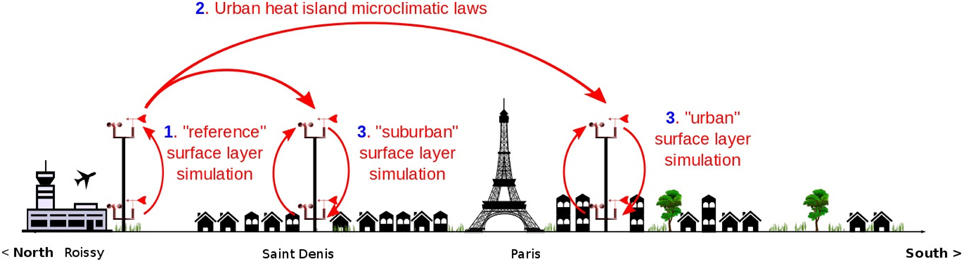
Figure 1. The three steps of the spatialized urban weather generator.

The domain chosen for this study is centered on the Paris city center, and has an extension of 100 km by 100 km. The grid mesh size is 2 km by 2 km (Figure 2). The domain size is chosen in order to be able to simulate the UHI over the city of Paris and its suburbs.

FIGURE 2

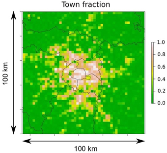
Figure 2. Domain of the simulation, represented by the town fraction. The domain size is 100 km by 100 km and the grid mesh 2 km by 2 km.

2.2. Meteorological Parameters Calculation by the Spatialized Integral Boundary Layer Model

2.2.1. Methodology

Above each grid mesh of the domain, a simplified integral boundary layer model is implemented. The energetic evolution of each boundary layer is calculated (see Section 2.2.2). The heat flux below the boundary layer is taken into account, thus inducing the local effect of the urbanization on the temperature and hence on the UHI. The influence of the nearest boundary layers is taken into account with the advection by the wind, thus allowing to represent the effect of the urbanization at the whole city scale on the UHI.

The CAT model only allows for calculating the temperature at a specific point, with a parametrization depending of this point. It is not adapted for a spatial vision of the UHI at the city scale. The urban weather generator uses a boundary layer model too but at the city scale. The energy budget is obtained by agreggating the whole city heat flux on a box of the size of the whole city. The UWG does not take into account local effects of the UHI. Moreover, the boundary layer height is always the same in the UWG. In this paper, a statistical model of the boundary layer height, depending of the built fraction, the wind speed, precipitation and cloud cover is implemented.

2.2.2. Heat Conservation in Boundary Layer Box Model

For each grid mesh, the boundary layer is considered as a box with a height z_i and a surface S corresponding to the grid mesh size. The energy budget is:

$\begin{array}{cc}\frac{dE}{dt}=H.S& (1)\end{array}$

with E the energy of the box advected and H the sensible heat flux at the bottom of the box calculated by the surface model. The temporal energetic variation of the integral boundary layer depends on the volume and temperature variation of the box (see Figure 3). During the day, the boundary layer height (BLH) is supposed to be spatially uniform (Stull, 1988; Lemonsu and Masson, 2002) and constant for each box and the energy budget is:

$\begin{array}{cc}T(t+dt)=T_{up}(t)+\frac{Hdt}{\rho c_p{z}_i}& (2)\end{array}$

with T_up(t) the upstream temperature that is advected on the grid mesh at time t + dt (see Section 2.2.3 for lagrangian advection details) and T(t + dt) the resulting temperature. The energy budget is computed at constant pressure. The effects of air expansion or compression on the boundary layer height are neglected. If T(t + dt) is less than the countryside temperature T_c, which is the temperature prescribed after the first step at 30 m at the operational weather station location, T(t + dt) is set at the value of T_c. With this law, which will be applied during the night too, it is assumed that the countryside temperature of the 2D temperature field will follow the forcing air temperature.

FIGURE 3

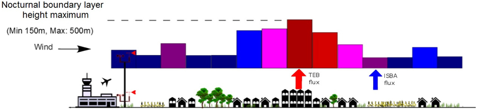
Figure 3. Energy budget for each grid mesh with a 2D lagrangian advection model.

During the night, the upstream box and the grid mesh box may not have the same height (see the boundary layer height prescription subsection). Two cases have to be considered and are described in Figure 4. If the upstream box is higher than the grid mesh box (z_i < z_iup), we consider that the air over the height of the grid mesh box is escaping (a). The energy budget is made only on the volume of the grid mesh (b). If the grid mesh box is higher than the upstream box (z_i > z_iup), we have to consider a larger volume for the upstream box. The missing part of the upstream box should have the same volume as the grid mesh box. Its temperature is considered to be at the countryside temperature (a'). The upstream temperature is in this case modified as:

$\begin{array}{cc}{T}_{up}^{\prime }(t)=T_{up}(t)(\frac{z_{iup}}{z_i})+T_c(t)(1-\frac{z_{iup}}{z_i})& (3)\end{array}$

FIGURE 4

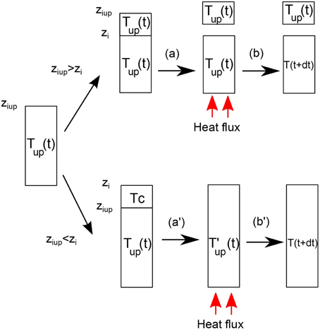
Figure 4. Description of the boundary layer model.

Finally, the nighttime energy budget is:

$\begin{array}{cc}T(t+dt)=T_{up}(t)(\frac{min(z_{iup},z_i)}{z_i})+T_c(t)(1-\frac{min(z_{iup},z_i)}{z_i})+\frac{Hdt}{\rho c_p{z}_i}& (4)\end{array}$

with z_iup the upstream BLH.

After sunrise, the increase of the BLH has to be reproduced in order to attenuate the nighttime urban heat island. This is achieved by supposing a mixing with the air above the nocturnal boundary layer. That air originates from the countryside boundary layer, and then is supposed to be at the countryside temperature. The mixing is performed with a time constant τ = 1800 s, representing the characteristic time for the boundary layer growth. The energy budget, initially drive by Equation (2) for daytime, becomes for the 2 h after sunrise :

$\begin{array}{cc}T(t+dt)=\frac{dt}{\tau }{T}_c(t)+(1-\frac{dt}{\tau })T_{up}(t)+\frac{Hdt}{\rho c_p{z}_i}& (5)\end{array}$

2.2.3. 2D-Advection Scheme

Contrary to the UWG, a lagrangian advection model is used to account for the wind effect. An eulerian advection model has been tested too but the lagrangian model has a better numerical stability with the same results. The upstream temperature T_up(t) is the temperature at the distance L = V_wind.dt from the center of the grid mesh. It is calculated with a bilinear interpolation with the temperatures of the four nearest grid mesh to the position of the upstream box (see Figure 5). If a grid mesh is located outside of the domain, the countryside temperature T_c is applied.

FIGURE 5

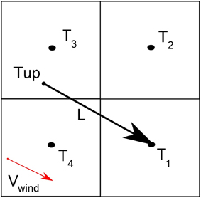
Figure 5. Lagrangian advection model. The upstream temperature T_up is calculated with a bilinear interpolation of T₁, T₂, T₃ and T₄.

The wind speed depends on the roughness length of the grid mesh (Grimmond and Oke, 1999). Considering a roughness length of 1 m in the city and 10 cm in the countryside, with a logarithmic law for the wind, a ratio $r_{wind}=\frac{V_{city}}{V_{country}}=0.6$ is obtained. This ratio is applied with a linear law on town fraction f_town between 0.3 and 0.7:

$\begin{array}{cc}\{\begin{array}{l}{r}_{wind}=1for{f}_{town}<0.3\\ r_{wind}=0.6for{f}_{town}>0.7\\ r_{wind}=-f_{town}+1.3elsewhere\end{array}& (6)\end{array}$

2.2.4. Urban Breeze

The wind in the model is the superposition of the synoptic wind and of the urban breeze. The synoptic wind is the direction and the speed of the wind calculated at the operational measurement weather station at 30 m and is applied at each grid mesh. To the synoptic wind, an urban breeze is added with the formulation of Hidalgo et al. (2010). The urban breeze maximum is:

$\begin{array}{cc}V{b}_{max}=\frac{g}{T_c}\frac{z_{i}max(H_{urb}-H_{coun},0)}{c_p\rho }& (7)\end{array}$

with H_urb the total town heat flux integrated all over the town fraction, H_coun, the recalculated country heat flux fitting the forcing air temperature evolution (see Section 2.2.6 for details), c_p the heat capacity at constant pressure, g the acceleration due to gravity, z_i the boundary layer height, calculated as z_imax in Section 2.2.5. In order to spatialize the urban breeze, we consider that the urban breeze direction is oriented to the city center. The urban breeze norm depends on the distance Xdist of the grid mesh center to the city center as defined in the following equations:

$\begin{array}{cc}\{\begin{array}{l}Vb=V{b}_{max}forXdist<0.25Ra\\ Vb=0forXdist>0.5Ra\\ Vb=V{b}_{max}\frac{Xdist}{0.5Ra}-2V{b}_{max}elsewhere\end{array}& (8)\end{array}$

with Ra the characteristic diameter of the city studied.

2.2.5. Boundary Layer Height Prescription

During the day, the boundary layer is the same on each grid mesh and is fixed at 1000 m. During the night, it appears with a 1 year MesoNH simulation (see Section 3.1 for details) that the BLH depends on the built fraction f_bld of the grid mesh. The nocturnal BLH maximum z_imax is obtained in the city center, where the built fraction is maximal and it appears that the BLH in the countryside is on average a quarter of the maximal BLH. Thus, the BLH is at night calculated as:

$\begin{array}{cc}{z}_i=\frac{z_{imax}}{4}+\frac{3f_{bld}{z}_{imax}}{4max(f_{bld})}& (9)\end{array}$

z_imax depends on the synoptic conditions (wind speed, cloud cover and precipitation), given by the forcing files. In the boundary layer model, z_imax depends on the wind speed. A statistical relation for the dependence of the boundary layer height has been extracted from a 1 year MesoNH simulation over Paris. This simulation will be used as a reference simulation for the validation of the SUWG but here it is used in order to prescribe the boundary layer height for the energy budget. A linear regression on the nocturnal boundary layer height in the city center of Paris (where the built fraction is maximal) at 3:00 UTC (in order to be at night all year long) in function the wind speed V_s gives a coefficient of correlation of 0.67 and the following relationship:

$\begin{array}{cc}{z}_{imax}=max(46V_s+53,150)& (10)\end{array}$

Moreover, if the cloud fraction is higher than 75% or if it rains or snows during the night, z_imax is set to 500 m, from the beginning of the precipitation to the end of the night. This statistical relation is very important in the SUWG because it will contribute to reproduce the seasonal variations of the UHI. Note that only the boundary layer height is prescribed statistically in the SUWG. The major part of the SUWG (the energy budget and the wind advection) is physically-based, so that the SUWG could reproduce the results of a meteorological mesoscale model.

2.2.6. Surface Fluxes Simulation

In the SUWG, the surface heat flux H is the weighted sum of the urban heat flux prescribed by TEB model H_teb and the country heat flux H_c:

$\begin{array}{cc}H=f{H}_{teb}+(1-f)H_c& (11)\end{array}$

with f the town fraction of the grid mesh. The urban flux heats locally the boundary layer. Then this heating is spatially distributed at the city-scale with the 2D-advection model. Thus, the UHI is higher in the city center than in a little town in the suburbs which could have locally the same urbanization. This outlines and models the role of the upstream urbanization for the UHI (Zhang et al., 2011). The UHI therefore affects the surface fluxes and the surface fluxes affects the UHI.

The countryside flux H_c is:

$\begin{array}{cc}{H}_c=H_{coun}+H_{isba}-max(H_{isba})& (12)\end{array}$

H_c represents the effect of the surface heating/cooling on the air temperature through surface energy fluxes, but not only. Indeed, the air temperature does not evolve solely due to the surface fluxes. Another main driver of the air temperature is the synoptic evolution of the air masses. Here, one has to ensure that our energy budget equation, in the countryside, follows the observed air temperature evolution. Consequently the heat flux entering in the box energy budget (for the countryside), is primarily constructed from the observed countryside temperature, with the first right-hand-side term H_coun defined as:

$\begin{array}{cc}{H}_{coun}=\frac{(T_c-T_{old})\rho c_p{z}_i}{dt}& (13)\end{array}$

with ρ the air density, c_p the heat capacity at constant pressure of the air, dt the time step, T_c the countryside temperature at the new time step, T_old the temperature at the previous time step and z_i the boundary layer height. This flux allows to take into account all effects affecting the countryside air temperature, including the synoptic conditions. Note that the synoptic conditions will also impact the urban air temperature, since the countryside air will be advected above the city.

However, we also wish to represent, when possible, the local effects due to different rural landscapes, such as forests or crops, that produce different heat fluxes and then potentially different temperature pattern within the simulation domain. In order to do this, we add in Equation (12) to H_coun a variability term computed by the ISBA surface model, that is able to simulate the variation of the surface heat fluxes.

2.2.7. Limits of the Methodology

One of the limits of the methodology is the attribution of all the measured parameters of the operational weather station at each grid mesh. It could be a problem for precipitation for example. During a night or a day for precipitation can be very local. Considering a single operational station as representative of the synoptic conditions is a strong hypothesis. How to reduce the error caused by this hypothesis will be discussed in the next part.

3. Results

3.1. Model Intercomparison

The reference simulation is computed with a full atmospheric model, MesoNH used for the research project CO2-MegaParis (Lac et al., 2013). MesoNH integrates effects of radiation, turbulence, clouds and shallow convection on the atmosphere. The atmosphere is divided in 46 levels vertically (the resolution is minimum near the surface and 2 km at the top of the domain above 20 km). As for the SUWG, the surface model of MesoNH is SURFEX, including TEB and ISBA. The simulation is a 1 year simulation (from 1 August 2010 to 31 July 2011) with a 2 km horizontal resolution over Paris and its suburbs. The reference simulation and the simulation with the SUWG are computed on the same grid. Each day of the reference simulation is simulated by a single run, initialized and coupled with Meteo France forecast model. In order to compare the UHI effect only, the synoptic effect is removed from the reference simulation with a method described in Annex 2 in Supplementary Materials.

To analyze the impact of the location of the rural boundary layer atmospheric data, that is used in step 1 to afterwards force the spatialized 2D integral boundary layer model (step 2), four operational weather stations have been chosen in four different places in Paris rural suburbs: Toussus-Le-Noble airport (TOU), in the south-west, Roissy airport (ROI) in the north-east, Orly airport (ORL) in the south-east and Pontoise airport (PON) in the north-east.

Six simulations are computed over a year: one with data from each stations (TOU, ROI, ORL, and PON), one is performed with data resulting from the average data of the four stations (MEAN) and the last one is a simulation with the average data but without taking account the SUWG (NoSUWG): the two dimensional forcing of the SURFEX model is made with homogeneous forcing files with an unique countryside temperature imposed over the whole domain.

In order to study the UHI at 2 m on the domain, the temperature at 2 m, computed by the surface model SURFEX, step 3 of the SUWG, with the forcing data resulting from step 2 of the SUWG, is considered. The UHI at 2 m in Paris is defined as the average of the temperature of the grid mesh points inside Paris from which the countryside temperature is subtracted. The countryside temperature is defined as the average of the grid mesh points with a 0% town fraction located at 30 km and more of the center of Paris. For the validation, the UHI at 2 m at 3:00 UTC in Paris is compared in each simulation with the reference simulation.

3.1.1. Results Over 1 Year

The scores of the simulations over a year are presented in Table 1 and Figure 6. Without the SUWG (simulation NoSUWG), the UHI computed is too weak for the highest values of UHI. With the UWG, the UHI is too high for every seasons, because of the fixed values of the boundary layer height. The mean bias error is negative and the largest in magnitude of all simulations. This shows the necessity to simulate the city-scale component of the UHI, as with the SUWG. Three simulations (TOU, PON, and ORL) have a too high mean bias error (MBE), i.e., more than 0.2 K. This is due to some days where the simulation gives UHI larger than 6 K when the reference is smaller than 5 K. These days, the synoptic conditions are not homogeneous. The weather at these stations is not representative of the weather at the domain scale. The ROI simulation gives too small values. The location of the forcing point is then important. Consequently we run a simulation with the average of all the forcing files (MEAN simulation). The best scores are obtained by this simulation with a mean bias error (MBE) of −0.04 K and a root mean square error (RMSE) of 0.83 K. The extreme values of the other simulations are corrected: these values were due to meteorological data which were not representative of the synoptic conditions. In the following sections of the article, one will consider only the MEAN simulation.

TABLE 1

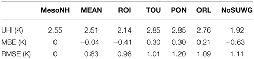
Table 1. Statistical evaluation of the predicted urban heat island at 2 m in Paris in comparison with a reference simulation MesoNH.

FIGURE 6

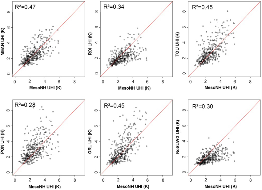
Figure 6. Comparison between simulation with the SUWG and MesoNH for the Paris UHI at 2 m at 3:00 UTC over a year for each forcing points and without the SUWG (NoSUWG).

3.1.2. Seasonal Results

In order to validate the SUWG, the seasonal results are plotted in Figures 7, 8 and the scores are presented in Table 2. For each season, the MBE and the RMSE are satisfactory. The summer has the lowest UHI this year because of terrible weather conditions on Paris area and this is well reproduced by the generator. The choices for the boundary layer height depending on the precipitation, wind speed and cloud cover fraction are relevant. The spatial extension of the UHI is well reproduced for each season.

FIGURE 7

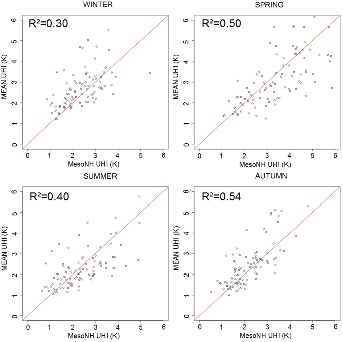
Figure 7. Comparison by season of the UHI at 2 m at 3:00 a.m. UTC in Paris computed by the SUWG forced with an average of data files from four different airports around Paris and a full atmospheric model MesoNH simulation.

FIGURE 8

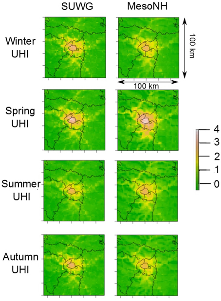
Figure 8. Comparison by season of the UHI at 2 m computed by the SUWG forced with an average of data files from four different airports around Paris and a full atmospheric model MesoNH simulation.

TABLE 2

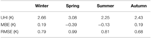
Table 2. Statistical evaluation of the predicted urban heat island at 2 m in Paris wit with the SUWG in comparison with a reference simulation MesoNH with the MEAN simulation for each season.

3.1.3. Comparison with the UWG

A simulation with the UWG and the average data from the four airports has been performed. The MBE and the RMSE between the UWG and MesoNH are respectively 0.35 K and 1.01 K. These values are higher than the values given by the SUWG. The main default of the UWG is its fixed values of the boundary layer height, which gives too high values of UHI in all seasons. The MBE between the UWG and MesoNH is higher than 0.2 K for each season (0.24 K in winter, 0.36 K in spring and summer and 0.44 K in autumn).

3.1.4. Daily Results

Day by day, the shape of the UHI is well reproduced if the wind at the reference station is representative of the synoptic conditions. Such a representative day, the 29th May is illustrated in the Figure 9. In both simulation the wind comes from the west. The spatial extension to the east of the UHI is the same with the SUWG and MesoNH. The advection model and the boundary layer height model are well parametrized. However, this also shows one of the weakness of the model. If the wind at the operational weather station is not representative of the synoptic conditions, the spatial extension of the UHI could be wrong.

FIGURE 9

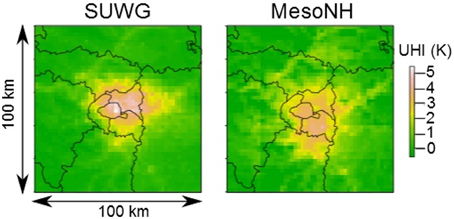
Figure 9. Comparison of the UHI at 2 m in Paris on the 29th of May computed by the SUWG with an average of data files from four different airports around Paris and a full atmospheric model MesoNH simulation.

3.1.5. Results for High UHI

Statistics have been performed on night with a UHI larger than 4K (39 nights during the year of simulation). The MBE between the UWG and MesoNH is −0.5 K and the RMSE 1.3 K for an average MesoNH UHI of 4.73 K. By comparison, without the UWG, the MBE, and the RMSE are respectively 2.2 K and 2.4 K. The SUWG reproduces well the high UHI episodes and is necessary to reproduce these episodes. Heat waves impact studies on cities and its inhabitants can therefore be modeled by the SUWG.

3.2. Comparison with Data

In order to validate the SUWG against operational data, in addition to the full atmospheric model, 31 operational measurement stations in the Paris area are used: 28 in the countryside (in blue dots), two in the near suburb of Paris (S1 in Courbevoie in and S2 in Saint-Maur-des-Fosses in red) and one in Paris (Montsouris park, P in red), see Figure 10.

FIGURE 10

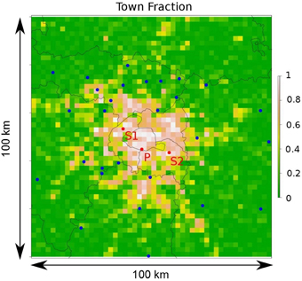
Figure 10. Localization of the operation weather station for the model validation. The blue dots represent the station required to calculate the countryside temperature. The red dots are the station needed for the validation of the UHI in the city.

Here, the countryside temperature is defined as the mean temperature of the 28 countryside stations. For the models (SUWG and MesoNH), the countryside temperature is the mean temperature of the 28 grid meshes containing the stations and the temperature for Paris and the suburb is the temperature of the grid mesh containing the stations. Note that for this validation, the synoptic signal has not been removed from the MesoNH simulation as in Section 3.1. The results are presented in Table 3 and Figure 11. The mean bias error and the root mean square error are similar between the SUWG and the full atmospheric model for the temperature inside the city and in its suburbs. The full atmospheric model has a better RMSE and R² in both case, but the scores of the SUWG are comparable to MesoNH. One reason for the too high MBE and low R² for both simulations is that the stations are located in parks, which are colder places than the built areas and not representative of the grid mesh in which they are located.

TABLE 3

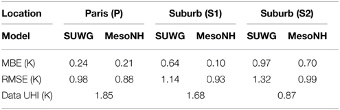
Table 3. Comparison of the scores of the nighttime urban heat island at 2 m in Paris and its suburbs given by the models (MesoNH and SUWG) with the data from measurement points (Mean Bias Error (MBE) (Model–Data) and Root Mean Square Error (RMSE) in K).

FIGURE 11

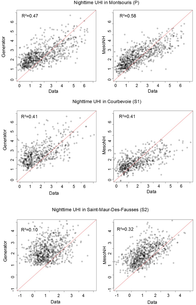
Figure 11. Comparison of the UHI at 2 m in Paris during the night (0:00 and 3:00 A.M. UTC) over a year of the data of three operational weather stations with simulations computed by the SUWG forced with an average of data files from four different airports around Paris and a full atmospheric model MesoNH simulation.

In Figure 12, the evolution of the temperature at the (P) station is represented in November and in May. This confirms that the generator gives an accurate representation of the temperature and the urban heat island in May when the amplitudes of temperature are important and in November when the diurnal cycle is less important.

FIGURE 12

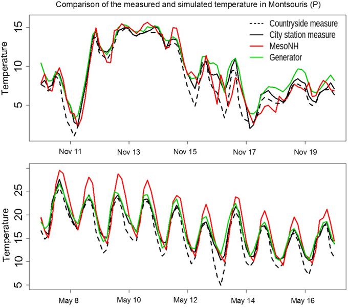
Figure 12. Temporal evolution of the temperature measured in the countryside (in black dashed lines), in the city at the Montsouris station (in black), simulated by the generator (in green) and by MesoNH (in red) in November and May.

4. Discussion

A new urban weather generator has been developed from the model developed by Bueno et al. (2013). The spatialized urban weather generator works with only one forcing point, coming from meteorological weather station outside of the city. However, it has been shown that for better simulations and a better representativeness of the synoptic conditions, an average of different stations around the area studied gives better results. First, the data from the operational weather stations is extrapolated at 30 m above the canopy layer. Then, the UHI is calculated on a grid above the mean height of the buildings by a simple boundary layer model. The boundary layer height is prescribed by a statistical model depending on the meteorological conditions and the built fraction of each grid mesh. Then an energy budget is solved in each boundary layer box with the heat flux provided by a surface model (here SURFEX, including ISBA, and TEB model) and a two dimensional lagrangian advection model. This methodology allows to simulate the intimate link between UHI and the surface fluxes of the urban area. Finally the meteorological parameters calculated at 30 m force the surface model, in order to obtain for example temperature at 2 m. The SUWG is therefore adapted for building energy consumption studies or pedestrian comfort studies. The generator has been validated against a 1 year simulation over the Paris area with the full atmospheric model MesoNH and against data of three measurement points in Paris and its near suburbs. The comparison between the SUWG and MesoNH provides accurate results and better score than the previous version, the UWG. However, the comparison of both models with the data from operational weather stations provides modest results. This is due to the location of the operational weather stations in Paris, which are often located in parks and are not representative of the 4 km² grid mesh. The SUWG model results have to be compared with data from a station representative of an urban temperature. The model has been also validated on each season. Consequently long term or seasonal urban studies can be performed with the SUWG. The interaction between the surface model and the boundary layer model will allow for studying for urban planning scenarios because the UHI calculated above the mean level of the building depends on the description of the surface. The SUWG has only been studied on one city (Paris), surrounded by plains. We recommend further SUWG model evaluation for cities beyond the Paris agglomeration. Moreover, a lot of mega-cities are coastal cities or surrounded by mountains. The SUWG has to be adapted in order to take into account the sea breeze or effects of orography.

Conflict of Interest Statement

The authors declare that the research was conducted in the absence of any commercial or financial relationships that could be construed as a potential conflict of interest.

Supplementary Material

The Supplementary Material for this article can be found online at: https://www.frontiersin.org/article/10.3389/feart.2015.00027/abstract

References

Belcher, S., Hacker, J., and Powell, D. (2005). Constructing design weather data for future climates. Build. Serv. Eng. Res. Technol. 26, 49–61. doi: 10.1191/0143624405bt112oa

CrossRef Full Text | Google Scholar

Bueno, B., Hidalgo, J., Pigeon, G., Norford, L., and Masson, V. (2013). Calculation of air temperatures above the urban canopy layer from measurements at a rural operational weather station. J. Appl. Meteorol. Climatol. 52, 472–483. doi: 10.1175/JAMC-D-12-083.1

CrossRef Full Text | Google Scholar

Bueno, B., Pigeon, G., Norford, L., and Zibouche, K. (2011). Development and evaluation of a building energy model integrated in the teb scheme. Geosci. Model Dev. Discuss. 4, 2973–3011. doi: 10.5194/gmdd-4-2973-2011

CrossRef Full Text | Google Scholar

Chang, C. H., and Goh, K. C. (1999). The relationship between height to width ratios and the heat island intensity at 22: 00 h for singapore. Int. J. Climatol. 19, 1011–1023. doi: 10.1002/(SICI)1097-0088(199907)19:9<1011::AID-JOC411>3.0.CO;2-U

CrossRef Full Text | Google Scholar

De Munck, C., Lemonsu, A., Bouzouidja, R., Masson, V., and Claverie, R. (2013). The greenroof module (v7.3) for modelling green roof hydrological and energetic performances within teb. Geosci. Model Dev. Discuss. 6, 1127–1172. doi: 10.5194/gmdd-6-1127-2013

CrossRef Full Text | Google Scholar

Erell, E., and Williamson, T. (2006). Simulating air temperature in an urban street canyon in all weather conditions using measured data at a reference meteorological station. Int. J. Climatol. 26, 1671–1694. doi: 10.1002/joc.1328

CrossRef Full Text | Google Scholar

Fortuniak, K. (2003). “An application of the urban energy balance scheme for a statistical modeling of the uhi intensity,” in Proceedings of the 5th International Conference on Urban Climate, Vol. 1 (Łódź), 59–62.

Grimmond, C., and Oke, T. R. (1999). Aerodynamic properties of urban areas derived from analysis of surface form. J. Appl. Meteorol. 38, 1262–1292. doi: 10.1175/1520-0450(1999)038<1262:APOUAD>2.0.CO;2

CrossRef Full Text | Google Scholar

Grimmond, C., and Oke, T. R. (2002). Turbulent heat fluxes in urban areas: observations and a local-scale urban meteorological parameterization scheme (lumps). J. Appl. Meteorol. 41, 792–810. doi: 10.1175/1520-0450(2002)041<0792:THFIUA>2.0.CO;2

CrossRef Full Text | Google Scholar

Gromke, C., Buccolieri, R., Di Sabatino, S., and Ruck, B. (2008). Dispersion study in a street canyon with tree planting by means of wind tunnel and numerical investigations–evaluation of cfd data with experimental data. Atmos. Environ. 42, 8640–8650. doi: 10.1016/j.atmosenv.2008.08.019

CrossRef Full Text | Google Scholar

Hidalgo, J., Masson, V., and Gimeno, L. (2010). Scaling the daytime urban heat island and urban-breeze circulation. J. Appl. Meteorol. Climatol. 49, 889–901. doi: 10.1175/2009JAMC2195.1

CrossRef Full Text | Google Scholar

Kershaw, T., Sanderson, M., Coley, D., and Eames, M. (2010). Estimation of the urban heat island for uk climate change projections. Buildi. Serv. Eng. Res. Technol. 31, 251–263. doi: 10.1177/0143624410365033

CrossRef Full Text | Google Scholar

Laaidi, M., Zeghnoun, A., Dousset, B., Bretin, P., Vandentorren, S., Giraudet, E., et al. (2012). The impact of heat islands on mortality in paris during the august 2003 heat wave. Environ. Health Perspect. 120, 254. doi: 10.1289/ehp.1103532

PubMed Abstract | CrossRef Full Text | Google Scholar

Lac, C., Donnelly, R., Masson, V., Pal, S., Riette, S., Donier, S., et al. (2013). Co 2 dispersion modelling over paris region within the co 2-megaparis project. Atmos. Chem. Phys. 13, 4941–4961. doi: 10.5194/acp-13-4941-2013

CrossRef Full Text | Google Scholar

Lemonsu, A., and Masson, V. (2002). Simulation of a summer urban breeze over paris. Boundary-Layer Meteorol. 104, 463–490. doi: 10.1023/A:1016509614936

CrossRef Full Text | Google Scholar

Lemonsu, A., Masson, V., Shashua-Bar, L., Erell, E., and Pearlmutter, D. (2012). Inclusion of vegetation in the town energy balance model for modelling urban green areas. Geosci. Model Dev. 5, 1377–1393. doi: 10.5194/gmd-5-1377-2012

CrossRef Full Text | Google Scholar

Martilli, A., Clappier, A., and Rotach, M. W. (2002). An urban surface exchange parameterisation for mesoscale models. Boundary-Layer Meteorol. 104, 261–304. doi: 10.1023/A:1016099921195

CrossRef Full Text | Google Scholar

Masson, V. (2000). A physically-based scheme for the urban energy budget in atmospheric models. Boundary-Layer Meteorol. 94, 357–397. doi: 10.1023/A:1002463829265

CrossRef Full Text | Google Scholar

Masson, V., Bonhomme, M., Salagnac, J.-L., Briottet, X., and Lemonsu, A. (2014). Solar panels reduce both global warming and urban heat island. Atmos. Sci. 2:14. doi: 10.3389/fenvs.2014.00014

CrossRef Full Text | Google Scholar

Masson, V., Le Moigne, P., Martin, E., Faroux, S., Alias, A., Alkama, R., et al. (2013). The surfexv7. 2 land and ocean surface platform for coupled or offline simulation of earth surface variables and fluxes. Geosci. Model Dev. 6, 929–960. doi: 10.5194/gmd-6-929-2013

CrossRef Full Text | Google Scholar

Moonen, P., Defraeye, T., Dorer, V., Blocken, B., and Carmeliet, J. (2012). Urban physics: effect of the micro-climate on comfort, health and energy demand. Front. Archit. Res. 1, 197–228. doi: 10.1016/j.foar.2012.05.002

CrossRef Full Text | Google Scholar

Noilhan, J., and Planton, S. (1989). A simple parameterization of land surface processes for meteorological models. Mon. Weather Rev. 117, 536–549. doi: 10.1175/1520-0493(1989)117<0536:ASPOLS>2.0.CO;2

CrossRef Full Text | Google Scholar

Oke, T. R. (1973). City size and the urban heat island. Atmos. Environ. 7, 769–779. doi: 10.1016/0004-6981(73)90140-6

CrossRef Full Text | Google Scholar

Park, H.-S. (1986). Features of the heat island in seoul and its surrounding cities. Atmos. Environ. 20, 1859–1866. doi: 10.1016/0004-6981(86)90326-4

CrossRef Full Text | Google Scholar

Prata, A. (1996). A new long-wave formula for estimating downward clear-sky radiation at the surface. Q. J. R. Meteorol. Soc. 122, 1127–1151. doi: 10.1002/qj.49712253306

CrossRef Full Text | Google Scholar

Remund, J. (2008). Quality of meteonorm version 6.0. Europe 6.

Google Scholar

Ren, Z., Wang, X., Chen, D., Wang, C., and Thatcher, M. (2012). Constructing weather data for building simulation considering urban heat island. Build. Serv. Eng. Res. Technol. 35, 69–82. doi: 10.1177/0143624412467194

CrossRef Full Text | Google Scholar

Stull, R. B. (1988). An Introduction to Boundary Layer Meteorology, Vol. 13. Springer Science & Business Media.

Google Scholar

Takahashi, K., Yoshida, H., Tanaka, Y., Aotake, N., and Wang, F. (2004). Measurement of thermal environment in kyoto city and its prediction by cfd simulation. Energy Build. 36, 771–779. doi: 10.1016/j.enbuild.2004.01.033

CrossRef Full Text | Google Scholar

Toparlar, Y., Blocken, B., Vos, P., van Heijst, G., Janssen, W., van Hooff, T., et al. (2015). Cfd simulation and validation of urban microclimate: a case study for bergpolder zuid, rotterdam. Build. Environ. 83, 79–90. doi: 10.1016/j.buildenv.2014.08.004

CrossRef Full Text | Google Scholar

Wilcox, S., and Marion, W. (2008). Users Manual for TMY3 Data Sets. National Renewable Energy Laboratory Golden, CO.

Google Scholar

Zhang, D.-L., Shou, Y.-X., Dickerson, R. R., and Chen, F. (2011). Impact of upstream urbanization on the urban heat island effects along the washington-baltimore corridor. J. Appl. Meteorol. Climatol. 50, 2012–2029. doi: 10.1175/JAMC-D-10-05008.1

CrossRef Full Text | Google Scholar