A new model for global glacier change and sea-level rise

1. Introduction

The ongoing and future retreat of glaciers around the globe is of major concern in light of direct implications for sea level, water resources, natural hazards and the human perception of mountains as a recreational environment (IPCC, 2013). Although glaciers outside the two ice sheets in Greenland and Antarctica contain less than 1% of all land ice, they are presently major contributors to sea-level rise (Kaser et al., 2006; Meier et al., 2007; Gardner et al., 2013). Glaciers react sensitively to changes in climate forcing and are expected to significantly recede over the next decades due to past and anticipated future atmospheric warming (Raper and Braithwaite, 2006; Radić and Hock, 2011; Marzeion et al., 2012; Marzeion et al., 2014).

While numerous studies have projected the twenty-first century evolution of individual glaciers, global-scale modeling of the roughly 200,000 glaciers worldwide remains challenging. This is mainly due to a scarcity of accurate data for model initialization and calibration, as well as difficulties in correcting for biases in climate input data in complex mountainous terrain. During the last 10 years only six global-scale models have been reported in the literature (see Radić and Hock, 2014, for a review). Forced by 8 to 15 Global Circulation Models (GCMs) and different emission scenarios, multi-model means of projected glacier mass loss by 2100 vary between 102 and 242 mm sea-level equivalent (SLE). These highly simplified models either directly calculate the transient surface mass balance using the degree-day method (Radić and Hock, 2011; Marzeion et al., 2012; Hirabayashi et al., 2013; Bliss et al., 2014; Radić et al., 2014), adopt a sensitivity approach (Slangen et al., 2012) or perturb equilibrium line altitudes (ELAs) according to temperature anomalies (Raper and Braithwaite, 2006). Giesen and Oerlemans (2013) calibrated a distributed energy-balance model to 89 glaciers in different climatic regions and upscaled the results to all glaciers globally. Only the models by Marzeion et al. (2012) and Radić et al. (2014) calculate the evolution of each individual glacier worldwide in response to transient temperature and precipitation scenarios.

Although the previous models provide first-order approximations of future glacier mass loss, they suffer from a number of shortcomings. Lacking global-scale ice thickness data, models have relied on scaling relations (often volume-area or volume-length scaling) to account for the dynamic response to modeled mass change, hence strongly simplifying the geometric adjustments caused by glacier dynamics. These approaches account for variations in glacier length but in a highly simplistic fashion, and also neglect changes in surface elevation. However, accurately modeling the glacier's geometric adjustment is crucial for capturing elevation-mass-balance feedbacks (e.g., Oerlemans et al., 1998; Huss et al., 2012; Trüssel et al., 2015).

Furthermore, none of the applied global glacier models account for frontal ablation of marine-terminating glaciers (dominated by mass loss due to calving and submarine melt). Roughly 30% of the world's glacier area presently drains into the ocean (Gardner et al., 2013) but only a few large-scale estimates of frontal ablation of glaciers outside the ice sheets exist (e.g., Błaszczyk et al., 2009; McNabb et al., 2015). It is evident that frontal ablation can be an important component of the glacier mass budget and is susceptible to significant changes within short time periods (Meier and Post, 1987; Osmanoglu et al., 2014). In addition, in many regions the refreezing of meltwater and rain in a glacier's firn layer is an important mass balance component, which may experience substantial changes in a warming climate (Pfeffer et al., 1991). However, previous global glacier models either do not incorporate this effect or parameterize it using simple empirical relations.

Improved process-based models suitable for worldwide application are thus urgently needed to reduce the uncertainties in projecting the sea-level contributions due to glacier mass loss. Although many challenges remain, several new large-scale data sets have emerged in recent years (e.g., Huss and Farinotti, 2012; Gardner et al., 2013; Pfeffer et al., 2014) that allow more sophisticated models to be developed for global glacier projections.

Here, we present a novel model for calculating the evolution of glaciers at the global scale. The model simulates the surface mass balance for each elevation band of every single glacier of the globally complete Randolph Glacier Inventory (RGI, Pfeffer et al., 2014) using a temperature-index model. Refreezing of meltwater and rain is calculated based on modeled snow and firn temperatures. Frontal ablation at tide-water glacier termini is computed using a simple model for calving (Oerlemans and Nick, 2005). Changes in glacier extent and surface elevation are modeled based on parameterized typical elevation change curves along glacier centerlines and initial ice thickness distribution for all glaciers derived from the methods by Huss and Farinotti (2012).

The model is driven with monthly temperature and precipitation projections from 14 Global Circulation Models (GCMs) forced by three emission scenarios to provide an updated assessment of global and regional glacier contribution to sea-level rise over the twenty-first century. We focus on the partitioning of the mass budget into its major components of mass gain and loss, and perform a range of sensitivity experiments to investigate the robustness of our results.

2. Data

2.1. Glacier Area, Hypsometry and Thickness

The RGI provides a globally complete set of outlines for all glaciers outside the two ice sheets Greenland and Antarctica (Pfeffer et al., 2014). Here, we use the RGIv4.0 (Arendt et al., 2014) for which information on the acquisition dates of 90% of the inventoried glaciers has been included. We report results for the 19 primary RGI regions (Supplementary Figure 1) based on Radić and Hock (2010).

Surface hypsometry for each glacier is derived from intersecting the outlines with Digital Elevation Models (DEMs). Between 55°S and 60°N we use the Shuttle Radar Topography Mission (SRTM) DEM (Jarvis et al., 2008), and in high latitudes the Advanced Space-borne Thermal Emission and Reflection Radiometer (ASTER) GDEMv2.0 (Tachikawa et al., 2011). For glaciers in the periphery of Greenland, surface topography is extracted from the Greenland Ice Mapping Project (GIMP) DEM (Howat et al., 2014), and for the Antarctic and Subantarctic from the Radarsat Antarctic Mapping Project (RAMP) DEM (Liu et al., 2001). In this study, each glacier is discretized into surface elevation bands of 10 m.

For each glacier of the RGIv4.0 we calculate ice thicknesses for 10 m elevation bands following Huss and Farinotti (2012). Their approach is based on estimates of ice volume fluxes and the principles of flow dynamics, and yielded generally good agreement between calculated thicknesses and observations. Here, we also use point thickness information provided by Operation IceBridge (Allen et al., 2010/2015) for almost 1000 glaciers in the periphery of Greenland and Antarctica, as well as in the Canadian Arctic (Gärtner-Roer et al., 2014) to adjust calculated thicknesses. Point thicknesses were averaged over the glaciers' elevation bands and, where available, these averages replaced the modeled ice thicknesses. Smoothing was applied as necessary. Table 1 provides an updated estimate of glacier volume and sea-level equivalent for each of the 19 primary RGI regions.

TABLE 1

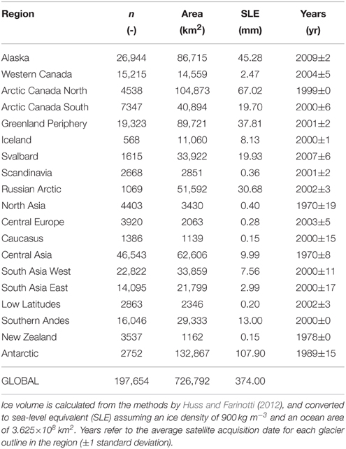
Table 1. Number of glaciers n and glacier area according to the Randolph Glacier Inventory (RGIv4.0) (Pfeffer et al., 2014).

For each elevation band, we also calculate slope, aspect, length and width (following Huss and Farinotti, 2012) from the above data sets for model input. Slope and aspect are needed for computing potential short-wave incoming radiation for a simplified energy-balance model used as an alternative approach in our sensitivity analysis (Section 6.6). Length and width are required for the frontal ablation model.

2.2. Glacier Mass Balance

2.2.1. Regional-scale Estimates for RGI Regions

For model calibration (Section 4.1) we use the consensus estimates of glacier mass changes for all RGI regions over the period 2003 to 2009 by Gardner et al. (2013), which are based on a combination of data from the Gravity Recovery and Climate Experiment (GRACE), the Ice, Cloud, and land Elevation Satellite (ICESat) and direct observations. This data set represents the most complete information on current glacier mass changes at large scales but does not resolve spatial variations within the regions, year-to-year variability, or seasonal components.

2.2.2. Annual and Seasonal Balance Time Series

For model validation we rely on surface mass-balance observations from in situ measurements on individual glaciers provided by the World Glacier Monitoring Service (WGMS, 2012). We use (i) glacier-wide annual balances for n = 198 glaciers, (ii) glacier-wide winter and summer balances (n = 132), (iii) annual and seasonal balance profiles (n = 124), and (iv) 2344 annual or seasonal point balances for 41 glaciers. To link the observations to the corresponding RGI glaciers an automated matching procedure is applied based on glacier coordinates and area. As the exact dates of the measurements are unknown for about two thirds of the entries of WGMS (2012) we assume annual mass balances to cover the hydrological year (1 October to 30 September) and the winter balance to refer to the period 1 October to 30 April. For the southern hemisphere dates are shifted by 6 months.

For model validation we also use 434 geodetic balances referring to individual glaciers or glacierized regions spanning over time intervals of 2–30 years (Cogley, 2009). Mass balance data are available for all RGI regions but the majority of observations refer to mid-latitude regions and generally small glaciers.

2.2.3. Frontal Ablation

To calibrate our frontal ablation model we use published regional-scale estimates of average frontal ablation rates. Estimates for entire RGI regions are available for Alaska (15.1 Gt a⁻¹, McNabb et al., 2015), Arctic Canada North (2.6 Gt a⁻¹, Van Wychen et al., 2014), Arctic Canada South (0.3 Gt a⁻¹, Gardner et al., 2011), Svalbard (6.7 Gt a⁻¹, Błaszczyk et al., 2009), the Russian Arctic (6.3 Gt a⁻¹, Glazovsky and Macheret, 2006; Moholdt et al., 2012), and the Southern Andes (17.5 Gt a⁻¹, Schaefer et al., 2015). In most cases these numbers are based on satellite-derived surface flow speeds at flux gates combined with estimates of ice thickness. No regional information on frontal ablation is available for the glaciers around Greenland and Antarctica, but for the latter region we consider estimates from the ice caps on King George Island and Livingston Island (Osmanoglu et al., 2013; Osmanoglu et al., 2014). For model validation we use mean frontal ablation rates derived for 27 individual tide-water glaciers in Alaska over the period 1985–2013 by McNabb et al. (2015).

2.3. Climate Data

The model is forced with monthly mean near-surface (2 m) air temperature and total precipitation using gridded climate products. For each glacier the data of the grid cell closest to its center coordinate is used.

2.3.1. ERA-interim Re-analysis

For model calibration we use the ERA-interim re-analysis of the European Centre for Medium Range Weather Forecasts (ECMWF) covering the period 1979 to present with a resolution of 0.5° × 0.5° globally (Dee et al., 2011). In addition, we also use air temperatures at eight pressure levels between 1000 and 500 hPa and their corresponding geopotential height to calculate monthly lapse rates in the free atmosphere for each grid cell. Daily 2 m air temperature series are used to calculate temperature variability for each month, which in turn is used to calculate degree-day sums (Section 3.1.2).

2.3.2. GCM Projections

Time series of monthly 2 m air temperature and precipitation for 14 GCMs from the Coupled Model Intercomparison Project Phase 5 (CMIP5) (Taylor et al., 2012) are used for the projections. All GCMs have a global coverage with a spatial resolution of between 1.1° × 1.1° to 2.8° × 2.8° (Supplementary Table 1). Data were downloaded for both historical runs (hindcast) and projections until 2099/2100. For some GCMs several ensemble members based on initialization with different atmospheric states are available. Here, we present the results referring to member r1i1p1 but for comparison we tested the effect of using different ensemble realizations (Section 6.1).

For each GCM the projections are driven by three different emission scenarios, the so-called Representative Concentration Pathways (RCP2.6, RCP4.5, and RCP8.5, IPCC, 2013). The RCPs are based on a range of projections of future population growth, technological development and societal responses (Meinshausen et al., 2011). Whereas, the RCP4.5 is an intermediate scenario with an additional radiative forcing of approximately 4.5 W m⁻² by the end of the twenty-first century, RCP8.5 is a high-emission scenario assuming rapid economical growth and only limited efforts to reduce emissions. For RCP2.6 emissions are expected to be drastically reduced toward the end of the century, resulting in radiative forcing of about +2.6 W m⁻² relative to pre-industrial levels (Meinshausen et al., 2011). Two GCMs (GFDL-CM3, INMCM4) do not provide results for RCP2.6.

2.3.3. Bias Correction

For each glacier a continuous monthly series of air temperature and precipitation 1980–2100 is generated based on the time series of the ERA-interim or GCM grid cell closest to the glacier. To correct for systematic biases between the two datasets we compare the mean monthly temperature and precipitation over the period 1980–2010. Additive (temperature) and multiplicative (precipitation) monthly biases are calculated. For the projection period, these biases—assumed to remain constant in time—are superimposed on the GCM series.

We further adjust the GCM air temperature data to account for differences in year-to-year variability between the re-analysis and the GCM time series. For each month m = [1, .., 12] the standard deviation of temperatures over 1980–2010 is calculated for both the re-analysis (σ_{ERA, m}) and the GCM series (σ_{GCM, m}). We then define the bias in temperature variability as Φ_m = σ_{ERA, m}∕σ_{GCM, m}. For each month m and year t of the projection period we correct interannual variability of GCM air temperatures T_{m, t} as

$\begin{array}{ll}{T}_{\mathit{\text{m,t, corrected}}}=\overline{T_{m,25}}+(T_{m,t}-\overline{T_{m,25}})·{\Phi }_m,& \left(1\right)\hfill \end{array}$

where $\overline{T_{m,25}}$ is the average temperature in a 25-year period around t. Accounting for the bias in interannual temperature variability is important to ensure validity of calibrated melt model parameters for the GCM-driven projections. Even with the same average temperature, a shift in variability between the hindcast and the forecast period can significantly alter the calibrated factors of empirical melt models (Hock, 2003; Farinotti, 2013). Our procedure corrects this shift while still allowing for future changes in temperature variability as given by the GCMs.

3. Global Glacier Model—GloGEM

We develop a new process-based model to calculate mass balance and associated geometric changes for each of the world's 200,000 glaciers. The model is henceforth referred to as GloGEM (Global Glacier Evolution Model). GloGEM computes all major components of the glacier mass budget. The climatic mass balance (i.e., the balance of snow accumulation, snow and ice melt, and refreezing) is calculated for every elevation band of each individual glacier with monthly resolution. For marine-terminating glaciers frontal ablation is computed at the end of each mass-balance year and added to the climatic balance to yield total annual mass change. The dynamic response of each glacier to mass changes is simulated based on an empirical relation describing thickness change as a function of normalized elevation range. The thickness, surface elevation and glacier extent are adjusted at the end of each mass-balance year. We do not account for the basal mass balance and the effect of supraglacial debris coverage on melt rates, which can be important in some regions. The main model components are described below.

GloGEM is calibrated and validated for the period 1980 to 2012 using ERA-interim data. It is then run with the downscaled GCM data until 2100 but the start year is individually chosen for each region to coincide with the average year which the RGI refers to (Table 1). This allows the model to account for glacier area changes between the RGI time stamp and the start of the RCP-forced GCM series (2013). We prefer using the historical GCM data instead of ERA-interim to avoid discontinuities at the transition between ERA-interim and GCM data. Mass-balance changes are then evaluated for all regions for the period 2010–2100.

Figure 1 shows an example of model output for a land-terminating and a marine-terminating glacier, illustrating the complex interplay between changes in area-elevation distribution, terminus retreat, frontal ablation and seasonal mass balance components. Supplementary Table 2 provides a list of all model parameters.

FIGURE 1

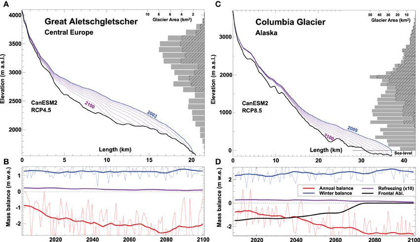
Figure 1. Modeled retreat of (A) Great Aletschgletscher (land-terminating), Central Europe, and (C) Columbia Glacier (tide-water glacier), Alaska, according to the CanESM2 GCM and RCP4.5/RCP8.5. Calculated glacier surfaces are shown in 10-year intervals. Area-elevation distribution in 100 m bins is shown for today (gray) and 2100 (hatched). (B,D) Temporal evolution of mass balance components. Yearly values of annual and winter surface balance are shown as thin lines. Thick lines refer to 11-year running means. Note that refreezing is enlarged by a factor 10.

3.1. Climatic Mass Balance

3.1.1. Accumulation

Accumulation is computed from precipitation by applying a temperature threshold T_s∕l = 1.5°C to differentiate between solid and liquid precipitation. All precipitation at temperatures T_s∕l ≤ T_s∕l − 1°C is assumed to fall as snow, while precipitation at T_s∕l ≥ T_s∕l + 1°C is assumed to be rain, with linear interpolation of the snow/rain ratio within this range. Precipitation in each elevation band i and month m is calculated by

$\begin{array}{ll}{P}_{i,m}=P_{\text{cell},\mathit{\text{m}}}·c_{\text{prec}}·(1+(z_i-z_{\text{ref}})·dP∕dz),& \left(2\right)\hfill \end{array}$

where P_{cell, m} (m) is monthly precipitation from the nearest grid cell of the gridded climate data and c_prec (no units) is a factor accounting for a potential bias in P. dP∕dz (m⁻¹) is a linear gradient relative to a reference elevation z_ref, here corresponding to that of the re-analysis grid cell. Since the DEM that underlies the re-analysis data only coarsely resolves the glacierized mountainous topography, the reference elevation z_ref falls below the glacier's lowest elevation for most glaciers. dP∕dz is set to a value of 1–2.5% per 100 m depending on the region as approximated from snow accumulation data (WGMS, 2012). For glaciers with an elevation range of >1000 m, precipitation is reduced with an exponential function over the uppermost 25% of the glacier's elevation bands to account for typically reduced air moisture content and increased wind erosion at higher elevation (e.g., Benn and Lehmkuhl, 2000), but P_{i, m} is constrained not to drop below 87.5% of maximum accumulation elsewhere on the glacier for that month.

3.1.2. Snow and Ice Melt

Snow and ice melt is calculated by the classical degree-day model (Hock, 2003) that relates melt a_{i, m} for each elevation band i and month m to positive degree-day sums. These sums can become inaccurate when monthly temperatures are close to the melting point. Therefore, we convert the monthly ERA-interim time series into daily series by superimposing a random variability that corresponds, for each month, to the standard deviation of daily ERA-interim temperatures over the period 1980–2010. Thus, the monthly temperature means are preserved but daily temperatures fluctuate. That way we account for melt in months with sub-freezing mean temperatures but occurrences of positive daily temperatures. Monthly melt is then computed as

$\begin{array}{ll}{a}_{i,m}=f_{\text{snow}∕\text{ice}}·{\displaystyle \sum _{d=1}^{d=D}}{T}_{i,d}^{+},& \left(3\right)\hfill \end{array}$

where f_snow∕ice (mm d⁻¹ K⁻¹) are the degree-day factors for snow or ice, and $T_{i,d}^{+}$ is daily positive mean air temperature, and D is the number of days per month. For firn surfaces we use the average of f_snow and f_ice. Air temperatures are extrapolated to all glacier elevation bands using a set of twelve constant monthly temperature lapse rates (Section 2.3).

3.1.3. Refreezing

Refreezing of rain and melt water is calculated for each elevation band from modeled snow and firn temperatures based on heat conduction:

$\begin{array}{ll}\frac{\partial T_{i,m}}{\partial t}=\frac{1}{c_h·\rho (z)}\frac{\partial }{\partial z}\left(\kappa \frac{\partial T_{i,m}}{\partial z}\right),& \left(4\right)\hfill \end{array}$

where c_h = 1.89 × 10⁶ J K⁻¹ kg⁻¹ is the heat capacity of ice, κ = 2.33 J s⁻¹ K⁻¹ m⁻¹ the conductivity and ρ(z) the density at depth z. The model is discretized in ten vertical 1 m layers; refreezing at more than 10 m below the surface is not considered. A constant density profile for snow and firn with an exponential increase in density with depth from 300 to 650 kg m⁻³ from the uppermost to the lowermost layer at 10 m is assumed for each elevation band and all glaciers, and for simplicity, remains constant with time. The heat conduction equation is solved explicitly in ten time steps per month to ensure numerical stability. Temperature T_{i, m} (in °C) of the uppermost layer is assumed to equal monthly mean air temperature. Equation (4) is only applied over winter (here defined by all months with total melt ≤2 mm w.e). The resulting englacial temperature profile of the last month satisfying this condition determines the maximum possible amount of refreezing r_{max, i} for the current mass-balance year, which is calculated as

$\begin{array}{ll}{r}_{\text{max},\text{i}}=\frac{-1}{L_f}{\displaystyle {\int }_0^z}\rho (z)c_h{T}_{i,m}(z)dz,& \left(5\right)\hfill \end{array}$

with L_f the latent heat of fusion. Outside the firn area (i.e., where bare ice underlies the winter snow pack) Equation (5) is integrated only over the thickness of the current snow cover. Actual refreezing r_{i, m} for each elevation band and each summer month is then determined from the sum of modeled melt and rain water assuming each month's melt/rain to refreeze until r_{max, i} is exhausted. The temperature profile at the beginning of each year's winter season is initialized with T(z) = 0°C in case total refreezing of the preceding year equals r_{max, i} (i.e., the cold content has been entirely eliminated). In all other cases the temperature profile is initialized with T(z) found at the end of the previous winter.

3.1.4. Surface Type

Surface type (snow/firn/ice) is needed for determining the degree-day factor (Equation 3) and for the refreezing model. In the first year of the modeling we initialize the end-of-summer surface type by prescribing firn above the median glacier elevation and bare ice below. We then update the surface type for each elevation band and month depending on the climatic mass balance. If the cumulative balance since the start of the mass-balance year is positive, surface type snow is assigned. If the cumulative balance is negative (i.e., all snow of the current mass-balance year has melted) either bare ice or firn is exposed. We assume the surface type to be firn if the elevation band's average annual balance over the preceding 5 years $\overline{B_{t-5}}$ has been positive. If $\overline{B_{t-5}}<0$ the surface type is ice. This simple approach accounts for spatio-temporal variations in firn area and related mass-balance feedbacks without the implementation of a full firn densification model.

3.2. Frontal Ablation

To account for frontal ablation of marine-terminating glaciers we employ a modified version of the approach proposed by Oerlemans and Nick (2005). The height of the calving front H_f is calculated as

$\begin{array}{ll}{H}_f=\text{max}(a_{\text{f}}{L}^{1∕2};\delta d),& \left(6\right)\hfill \end{array}$

where a_f = 0.7 m^1∕2 is a constant, L (m) is glacier length, δ is the ratio of water density to ice density, and d (m) is the water depth at the glacier terminus obtained from surface elevation and ice thickness. Annual frontal ablation F is computed as a function of H_f, d and width w of the calving front as

$\begin{array}{ll}F=\text{max}(0;kd{H}_{\text{f}})·w,& \left(7\right)\hfill \end{array}$

where k is a parameter (set to 2 a⁻¹ by Oerlemans and Nick, 2005).

Here we assume k to be linearly dependent on the average slope β_t (deg) of the glacier terminus (defined by the elevation bands between 0 and 100 m a.s.l.):

$\begin{array}{ll}k=k_0·{\beta }_{\text{t}}.& \left(8\right)\hfill \end{array}$

k₀ (deg⁻¹ a⁻¹) is assumed constant for all glaciers within each primary RGI region but values may differ among regions. Thus, region-specific characteristics can be taken into account. We tune the poorly constrained parameter k₀ for each of the 9 RGI regions that contain marine-terminating glaciers to maximize the agreement between calculated and observed regional-scale estimates of frontal ablation (Section 2.2). Additional frontal ablation due to glacier retreat is computed in the glacier geometry change module (Section 3.3).

3.3. Glacier Geometry Change

Glacier geometry including area, thickness and surface elevation of each band is updated in annual time steps using the mass-conserving retreat parameterization developed by Huss et al. (2010). In case of negative mass balance, the calculated annual glacier-wide mass change is redistributed across all elevation bands according to a non-dimensional empirical function that assumes no elevation change at the glacier's highest elevation and maximum elevation changes at the glacier terminus as typically observed on retreating or advancing glaciers (Jóhannesson et al., 1989; Arendt et al., 2002; Das et al., 2014). Normalized surface elevation change Δh is calculated as a function of the each band's elevation difference h_n to the lowest band normalized with the glacier's total elevation range by

$\begin{array}{ll}\Delta h={(h_{\text{n}}+a)}^{\gamma }+b·(h_{\text{n}}+a)+c,& \left(9\right)\hfill \end{array}$

where the coefficients a, b, c and γ (no units) are taken from Huss et al. (2010) and specified for three glacier size classes (0–5 km², 5–20 km², >20 km²). Integration of the surface elevation change over all elevation bands N must equal the total annual change in glacier mass ΔM:

$\begin{array}{ll}\Delta M={\rho }_{\text{ice}}·{\displaystyle \sum _{i=0}^{i=N}}{A}_i·f_{\text{s}}·\Delta h_i,& \left(10\right)\hfill \end{array}$

where A_i is the area of each elevation band i. The factor f_s scales the magnitude of the dimensionless ice thickness change pattern (Equation 9) and is chosen for each year such that Equation (10) is satisfied. The mean thickness H (m) of each elevation band is then updated according to

$\begin{array}{ll}{H}_{i,t+1}=H_{i,t}+f_{\text{s}}·\Delta h_i.& \left(11\right)\hfill \end{array}$

For elevation bands with H_{i, t+1} < 0, ice thickness is set to zero thus accounting for glacier retreat.

In addition, the width and area of each elevation band is adjusted assuming a parabolic cross-sectional shape of the glacier bed. The area A_{i, t+1} of elevation band i in year t is updated depending on the new ice thickness H_{i, t+1}, the initial area A_{i, t = 0} and initial thickness H_{i, t = 0} of the band as

$\begin{array}{ll}{A}_{i,t+1}=A_{i,0}·{\left(\frac{H_{i,t+1}}{H_{i,0}}\right)}^{0.5}.& \left(12\right)\hfill \end{array}$

This step requires caution as it may lead to mass “loss” or “gain” due to changing elevation band area. We account for this effect by correcting the resulting thickness and surface elevation in each band so that mass conservation is enforced. Sensitivity tests using either a rectangular or a triangular cross-sectional shape for all glaciers instead of a parabolic indicated that projected mass loss by 2100 may increase/decrease by 1–4%.

We extend the parameterization originally developed for glacier retreat to account for glacier advance. In case of positive glacier-wide mass balances, ice thickness is adjusted according to Equations (9–11). When the thickness increase exceeds a threshold set to +5 m a⁻¹ for at least one band, we assume glacier advance and move the excess ice volume of all elevation bands above this threshold downglacier, thus adding new band(s). The number of elevation bands added is determined by the excess volume, and the area and thickness of the added bands. The area of each added band is assumed to equal the average elevation-band area over h_term defined as the bands contained in the lowermost 20% of the glacier's elevation range. The thickness corresponds to that of the lowermost band from the previous time step. For the first new band we define A₀ and H₀ as the average of these variables over h_term. A₀ and H₀ are needed in subsequent years when the area and thickness of all bands, including the added ones, are adjusted according to Equation (12). We gradually increase A₀ and H₀ with each newly added band thus making each added elevation band wider than the previous one in order to avoid too rapid advances in case of prolonged positive mass balances. Our simplified advance scheme suffices for our purposes given that glacier retreat dominates in all regions.

We apply our parameterization for glacier geometry change to both land- and marine-terminating glaciers. For the latter, elevation bands with a surface below the floatation level are cut off (Trüssel et al., 2015), and the corresponding volume loss is added to the frontal ablation component computed by Equation (7).

3.4. Computing Sea-level Equivalent

We convert calculated glacier mass loss into sea-level equivalent SLE_ΔM by assuming an ice density of 900 kg m⁻³ and an ocean area of 3.625 × 10⁸ km² (Cogley et al., 2011). Here, we also account for the effect that ice presently located below sea level at marine-terminating glacier fronts already displaces sea water, and therefore has only a minor effect on sea-level change if melted. Although only a small fraction of the total glacier volume is presently grounded below sea level, this effect systematically reduces the contribution of glacier melt to sea-level rise (Haeberli and Linsbauer, 2013). For each year and each elevation band with grounded ice that is entirely lost, we compute the sea-level equivalent SLE_eff by

$\begin{array}{ll}SL{E}_{\text{eff},i}={\displaystyle \sum _{i=0}^{i=N}}{w}_i(h_i·\frac{{\rho }_{\text{ice}}}{{\rho }_{\text{water}}}-d_i),& \left(13\right)\hfill \end{array}$

where w_i is the width and h_i the thickness of elevation band i, ρ_ice and ρ_water the density of ice and water, N the number of elevation bands, with ice below sea level and d_i the mean depth of the ocean water in which the melted ice stood. For net mass loss in all other elevation bands SLE_{eff, i} equals SLE_{ΔM, i}. The same procedure is applied to lake-terminating glaciers, but only if the bed topography of the retreating front is below sea level. We assume that the lost ice volume is replaced by lake water and, hence, does not contribute to sea-level rise. This will also be the case for lakes forming at elevations above sea level. However, our datasets do not allow us to reliably detect those cases in an automated fashion.

Here, the sea-level equivalent due to glacier mass loss corrected for the effects of lost ice below sea level is referred to as SLE_eff to distinguish it clearly from SLE_ΔM derived only from glacier mass change and ocean area as typically done in previous studies (e.g., Marzeion et al., 2012; Radić et al., 2014). However, we note that more accurate estimates of actual sea-level rise from glacier melt must also consider processes such as flow of water into deep aquifers or endorheic basins, shoreline migration, changes in ocean area and isostatic adjustments to land and ocean surfaces.

4. Calibration and Validation

4.1. Model Calibration

4.1.1. Background

One of the biggest challenges of global glacier models is their calibration. Calibration is required as neither the downscaled meteorological variables describe the site-specific conditions accurately enough, nor is the glacier model able to resolve the complex processes for each of the 200,000 glaciers precisely. Most global glacier models have used in situ mass balance records as the main calibration data source (Radić and Hock, 2011; Giesen and Oerlemans, 2013). In some studies, model parameters were further fine-tuned to match estimates of regional mass changes derived from extrapolation of glacier observations (Radić et al., 2014). However, calibrating a global model to in situ mass balance data from individual glaciers is problematic. Direct observations are often restricted to rather small glaciers, and the regions with the largest ice cover are strongly undersampled.

We consider the mass balance estimates for all RGI regions for the period 2003–2009 presented by Gardner et al. (2013) as the most credible and comprehensive information on the global glacier mass budget presently available and utilize these data for model calibration. Mass balance observations from individual glaciers are used for model validation.

In order to calibrate a regional model to regional-scale mass-balance observations a common approach (e.g., Radić et al., 2014) is to tune parameters so that the sum of the modeled mass changes of all individual glaciers matches the region-wide observed mass change over the same period:

$\begin{array}{ll}\sum (\Delta M_g·A_g):=\Delta M_{\text{reg}}·\sum A_g,& \left(14\right)\hfill \end{array}$

where ΔM_g is the modeled specific glacier-wide mass change of each glacier g in m water equivalent (w.e.) and A_g is glacier area. ΔM_reg is the observed regional mass change in the same units. In this case, model parameters are assumed constant for all glaciers or may vary according to prescribed transfer functions (Radić et al., 2014). Modeled specific mass balances will differ from glacier to glacier due to spatially varying climate forcing and different area-altitude distributions.

Here we take a different approach. Each individual glacier's specific mass balance is forced to match the average regional specific balance during the same multi-year time period:

$\begin{array}{ll}\Delta M_g:=\Delta M_{\text{reg}}.& \left(15\right)\hfill \end{array}$

Hence, each glacier has a unique set of tuned model parameters. It is known that neighboring glaciers can show significantly different mass balances despite similar regional climate (e.g., Arendt et al., 2002; Moholdt et al., 2010). However, this approach ensures that each glacier's mass balance is constrained to a physically reasonable range, in contrast to the former approach where individual glaciers can have highly unrealistic balances although the modeled and observed regional balances match.

This is illustrated in Figure 2B where we applied both approaches to a subset of glaciers in Central Europe for comparison. As expected, for the latter approach the average balance rate of each glacier remains within the targeted range of –1.06±0.1 m w.e. a⁻¹ for the entire RGI region. In contrast, for the former approach (Equation 14) average balance rates vary considerably among the glaciers as typically seen within a glacierized region, but the standard deviation of 1.74 m w.e. a⁻¹ is substantially higher than indicated by direct observations. For more than 1000 glaciers in Switzerland, Fischer et al. (2015) report a standard deviation σ = 0.24 m w.e. a⁻¹ for geodetic mass balance over the period 1980–2010. Average in situ mass balances (WGMS, 2012) for all glaciers in the European Alps reveal σ = 0.34 m w.e. a⁻¹ for 1980–2010, and σ = 0.61 m w.e. a⁻¹ for 2003–2009.

FIGURE 2

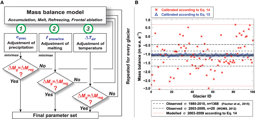
Figure 2. (A) Visualization of the calibration scheme. For each glacier the calibration steps 1, 2, and 3 are passed through sequentially until a final parameter set is found based on Equation (15). (B) Comparison of two possible methods (Equations 14, 15) to calibrate the model. Symbols refer to glacier-wide specific mass balance rates averaged over the period 2003 to 2009 for 100 randomly selected glaciers within the RGI region Central Europe. The solid horizontal line indicates the regional mass balance ΔM_reg± the allowed range (shaded) if Equation (15) is applied. Dashed and dash-dotted lines show observed standard deviations σ of average balance rates of n glaciers from two studies. Both methods yield nearly identical ΔM_reg but balance rates for the same glaciers differ strongly between the two calibration methods.

4.1.2. Climatic Mass Balance

In this study, we adopt the latter approach (Equation 15) and apply a three-step calibration procedure (Figure 2A) to determine the model parameters c_prec (Equation 2), f_snow and f_ice (Equation 3). The model is run over the calibration period 2003–2009 with initial estimates for the parameters c_prec = 1.5, f_snow = 3 mm d⁻¹ K⁻¹, f_ice = 6 mm d⁻¹ K⁻¹ based on literature values (e.g., Hock, 2003; Braithwaite, 2008). The module for glacier geometry change is disabled for the 6-year calibration period. If the calculated glacier-wide specific mass balance agrees with regional specific balance within a threshold set to ±0.1 m w.e. a⁻¹, the meteorological forcing series is considered to describe the climatic conditions for this glacier well, and no further changes to the parameter values are applied. If deviations are greater, c_prec is varied within reasonable bounds (0.8–2.0) until agreement is achieved (calibration step 1). We choose the bias in precipitation as primary calibration parameter as it is expected to be most poorly captured by the re-analysis data and to show large small-scale variability among nearby glaciers, e.g., due to wind drift and/or avalanches (e.g., Machguth et al., 2006). If no agreement is found within the tested range, c_prec is set to the value that resulted in the smallest deviation from ΔM_reg, and f_snow is varied between 1.75 and 4.5 mm d⁻¹ K⁻¹. f_ice is adjusted so that the ratio f_ice∕f_snow = 2 is preserved (step 2). If the target mass balance cannot be reproduced within these parameter ranges we assume that there is a systematic error in the temperature forcing data. Thus, in a final third step, we systematically shift the air temperature series by ΔT until agreement between the glacier's specific mass balance and the observed regional balance is achieved (step 3).

Overall, for one third of the glaciers agreement was found within calibration step 1, for one third within step 2 and for one third within step 3 (Supplementary Table 3). For most high-latitude regions (e.g., Arctic Canada, Russian Arctic), convergence was generally reached at step 3. For 2% of all glaciers the calibration procedure (Figure 2A) did not converge. For these mostly small glaciers we assigned regional average parameters.

4.1.3. Frontal Ablation

The frontal ablation model is tuned by varying the parameter k₀ (Equation 8) so that modeled regional frontal ablation rates are in agreement with observation-based estimates that are available over various time periods (see Supplementary Table 8). The tidewater glaciers are not calibrated individually. The glacier dynamics module is de-activated for calibration, i.e., glacier geometry is assumed constant to avoid non-linear run-away effects due to inaccuracies in modeled glacier terminus geometry. Hence, the modeled frontal ablation rates do not vary with time during calibration. For glaciers around Greenland and Antarctica k₀ is chosen based on values found for regions with similar glacier characteristics (Supplementary Table 4). The parameter k₀ appears to depend on regional precipitation totals, which is likely related to differences glacier flow dynamics that are not explicitly modeled in our approach.

4.2. Model Validation

The calibrated model is run for all glaciers over the validation period 1980–2012 using ERA-interim re-analysis data. Over this period we do not account for glacier geometry changes as the RGI only provides one temporal snapshot that mostly refers to the last decade (Table 1). Model results are validated against observations of glacier-wide annual balances, glacier-wide winter and summer balances, annual and seasonal balance profiles, seasonal point balances, geodetic balances and frontal ablation (refer to Section 2.2). By using the combined model for mass balance and geometry change we also utilize observed area changes from repeated glacier inventories for validation. The region-wide mass balances (Gardner et al., 2013) used for model calibration are independent from the validation data except for a few regions where direct mass balance observations over the period 2003–2009 were extrapolated to infer the regional mass change.

4.2.1. Annual and Seasonal Mass Balances

In general, we find good agreement between modeled and observed glacier-wide annual mass balances. The Root-Mean-Square Error (RMSE) is 0.73 m w.e. (n = 3148, Figure 3A), and the bias is close to zero. In a few regions, the absolute bias is larger reaching up to 0.5 m w.e. (Supplementary Table 4). Biases are expected to increase as the sample size decreases, as individual glaciers might not be representative of the regional balances used to calibrate the model. Modeled and observed balances for glacier elevation bands also agree well (Figure 3C). This indicates that the model is able to approximate the distribution of annual mass balance over the glaciers' elevation range in different climatic regimes without being calibrated to these data.

FIGURE 3

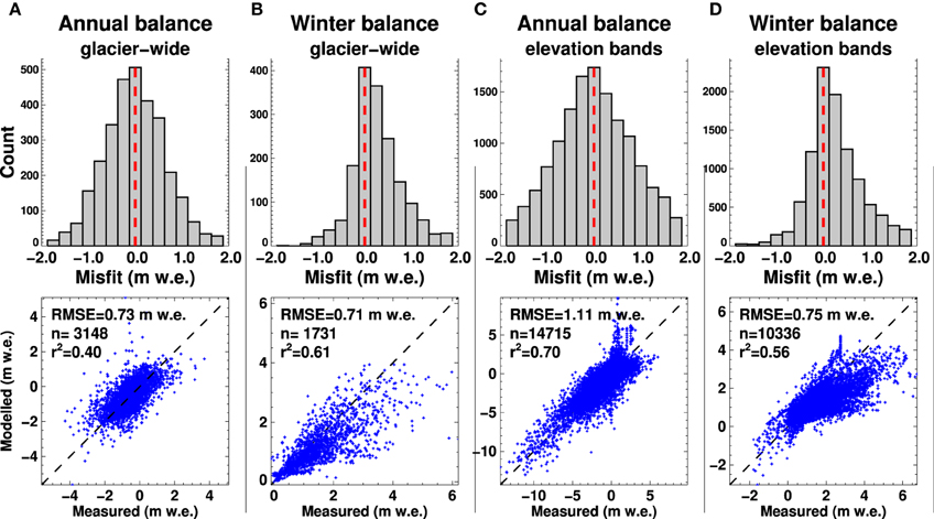
Figure 3. Model validation results using mass balance observations between 1980 and 2012 (WGMS, 2012): Frequency of misfits in bins of 0.25 m w.e. (observed minus modeled, upper panels) and scattergrams (lower panels) of modeled vs measured glacier-wide (A) annual balances, (B) winter balances, and (C) annual and (D) winter balances for individual elevation bands. Dashed red lines mark the zero misfit; the root-mean-square error (RMSE), the number of samples n, and the linear correlation coefficient r² are given in the lower panels.

The winter balances are less well reproduced with a tendency for the model to underestimate them in some regions (Figures 3B,D). Part of this bias might be due to differences in observation period length (stratigraphic vs fixed-date system, Cogley et al., 2011). Also, the seasonal components of mass change cannot be constrained by our calibration procedure since it tunes parameters to observed regional total balances rather than seasonally differentiated observations.

We also validate the model against seasonal point mass balances since these are unaffected by uncertainties in glacier-wide balance arising from extrapolating point measurements over the entire glacier surface. Model performance is satisfying for point balances from about 40 glaciers in different climatic regions with r²-values ranging from 0.4 to 0.9 (Supplementary Table 5).

4.2.2. Geodetic Mass Balance

We find good agreement between modeled and observed geodetic balances indicating that GloGEM is able to resolve regional differences in mass balance rates. Figure 4 shows that the misfit is less than 0.5 m w.e. a⁻¹ for 66% of the observations, or for 84% of the total area covered. For the remaining cases there is a tendency for the model to overestimate mass balance. This is particularly pronounced for small glaciers, whereas the bias for large glaciers is relatively small.

FIGURE 4

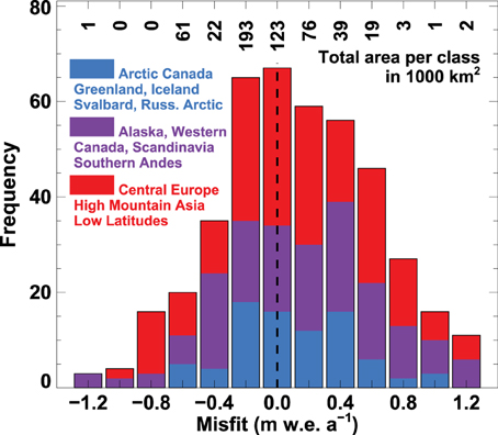
Figure 4. Model validation against 434 geodetic balances (Cogley, 2009): Frequency distribution of the misfit (observed minus modeled balance) in bins of 0.2 m w.e. a⁻¹. Results are distinguished for three large-scale regions dominated by ice caps (blue), polar mountain glaciers (purple) and mid-latitude glaciers (red). The total glacierized area covered by the observed geodetic balances is given for each bin in 1000 km². 2% of the misfits are beyond the plotted range.

4.2.3. Area Changes

We validate our model for adjusting glacier geometry by comparing modeled and observed area change rates from different regions with various climates and glacier types. The glacier model was run for each of the regions over the period covered by repeated inventories and geometry was annually updated. For most cases a satisfying agreement of observed and calculated glacier area change rate is found (r² = 0.66, n = 12). Also differences among the regions were adequately reproduced by the model (Supplementary Table 6).

4.2.4. Frontal Ablation

Regressing modeled and observed frontal ablation rates for the 27 Alaskan glaciers analyzed by McNabb et al. (2015) results in a correlation of r² = 0.73 (0.88) when including (excluding) Columbia Glacier whose unstable retreat during the validation period is difficult to capture by our simple model. For the three largest tide-water glaciers, the errors in simulated frontal ablation rates are +2% (Hubbard), −55% (Columbia) and +25% (Yahtse).

5. Results

5.1. Hindcast 1980–2012

The calibrated model was run for the period 1980–2012 using ERA-interim re-analysis data. For all glaciers globally we find specific mass balance rates decreasing from roughly –0.1 m w.e. a⁻¹ before the mid-1990s to about –0.5 m w.e. a⁻¹ over the last 5–6 years (Figure 5) corresponding to an overall glacier mass loss of 12.3 mm SLE_ΔM since 1980. The variability in mass balance among the individual regions is considerable. Whereas, an only slightly negative balance is found for glaciers in High Mountain Asia, a strongly fluctuating signal is revealed for Alaska, and rapidly increasing mass loss is modeled for the European Alps.

FIGURE 5

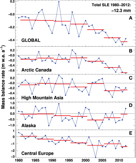
Figure 5. Modeled specific mass balance rates (including climatic balance and frontal ablation) based on ERA-interim data for (A) all glaciers globally, and (B–E) selected regions. Note that the scales differ among the panels. The horizontal bars show pentadal averages.

5.2. Glacier Volume Projections 2010–2100

Global glacier volume is projected to decrease by 25±6% for RCP2.6, 33±8% for RCP4.5, and 48±9% for RCP8.5 (multi-model mean ±1 standard deviation σ) by the end of the century. Substantial glacier volume reduction is found in all regions (Figure 6A). The global signal is dominated by the high-latitude glaciers where glacierized area is largest. The RCP4.5 multi-model mean indicates glacier volume losses of between –20% (Arctic Canada North, Antarctic and Subantarctic) and –90% (Central Europe, Low Latitudes). However, the spread among the individual GCMs for identical emission scenarios is substantial (Figure 6A), in particular for Svalbard, the Russian Arctic and Iceland. For Svalbard, projected volume changes vary between –12 and –91% (RCP4.5) indicating that the disagreement of future temperature and precipitation scenarios is considerable among the GCMs (Supplementary Figures 2–4). At the global scale, the HadGEM2-ES GCM results in the largest mass loss and INMCM4 in the smallest by the end of the century. The results from the CNRM-CM5 model are close to the multi-model mean (Supplementary Table 7).

FIGURE 6

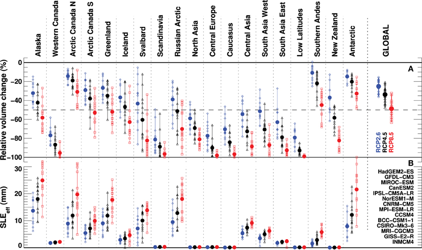
Figure 6. (A) Relative change in regional ice volume and (B) contribution to sea-level rise (SLE_eff) between 2010 and 2100 specified for all 14 GCMs (symbols) and RCP2.6 (blue), RCP4.5 (black), and RCP8.5 (red). The multi-model means are shown as filled circles. GCMs are listed in the order of modeled global SLE_eff (Figure 7).

5.3. Sea-level Equivalent Projections

Multi-model means of SLE_ΔM from all glaciers for 2010–2100 are 91±26 mm (RCP2.6), 123±30 mm (RCP4.5) and 178±33 mm (RCP8.5, Figure 7). In contrast to previous global glacier studies we account for the effect of glacier mass loss not contributing to sea-level rise if the lost ice volume is located below sea level (Equation 13). Until 2100 this effect reduces the projected glacier contribution by 11–14% (multi-model means for the three RCPs) and thus represents a non-negligible component. More than half of the reduction can be attributed to glaciers of the Antarctic and Subantarctic. We find a multi-model mean effective sea-level contribution (SLE_eff) of 79±24 mm (RCP2.6), 108±28 mm (RCP4.5) and 157±31 mm (RCP8.5, Figure 7, Table 2).

FIGURE 7

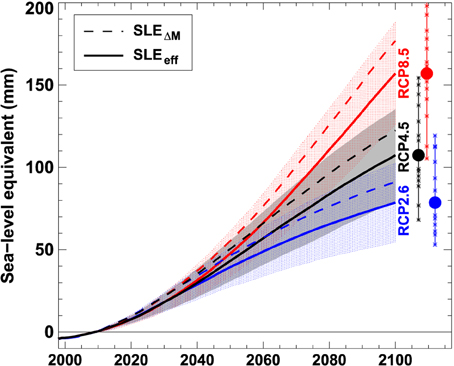
Figure 7. Multi-model means of projected cumulative global sea-level equivalent from glacier net mass loss relative to 2010 neglecting (SLE_ΔM) and accounting (SLE_eff) for the effect of ice displacing ocean water using three RCPs. The shading indicates ±1σ for SLE_eff from the 14 GCMs. Crosses show SLE_eff by 2100 for each GCM run; filled circles refer to multi-model means.

TABLE 2

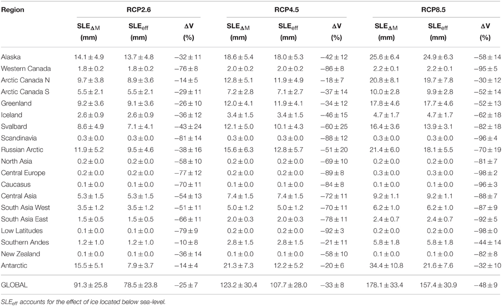
Table 2. Regionally differentiated glacier mass loss in sea-level equivalent (SLE_ΔM and SLE_eff), and glacier volume change ΔV for the period 2010–2100 (multi-model mean ±1σ).

The most important contributors to sea-level rise are the Canadian Arctic, Alaska, the Russian Arctic, Svalbard, and the periphery of Greenland and Antarctica (Figure 6B, Table 2, Supplementary Figures 5–10, Supplementary Table 9, Data Sheet 1). The timing and the magnitude of maximum rates of sea-level rise contribution from glaciers differ among the scenarios. For RCP4.5, the largest rates reaching 1.4 mm a⁻¹ (multi-model mean) are found around 2060. In contrast, peak rates occur around 2045 for RCP2.6 (1.1 mm a⁻¹), while they increase until about 2090 for RCP8.5 reaching 2.4 mm a⁻¹.

Bahr and Radić (2012) have emphasized the relevance of small glaciers to total ice volume and potential sea-level change. We have evaluated the mass loss of all glaciers according to size classes in order to determine the importance of small glaciers to global glacier wastage. Glaciers presently smaller than 1 km² make up for only 0.7% of total ice volume but account for 6.7% of SLE_eff during the period 2015–2025 (Figure 8) indicating that very small glaciers are a non-negligible component of global glacier change, at least in the near future. Over the next decade 28% of the sea-level contribution originates from glaciers smaller than 10 km² today. The relative importance of large glaciers (>100 km²) gradually increases toward the end of the twentyfirst century. This is explained by their growing imbalance with progressing warming, and because many smaller glaciers completely disappear by 2100. With future ice wastage it is likely that large glaciers will disintegrate thus resulting in the formation of new small glaciers. Our model does however not account for this process.

FIGURE 8

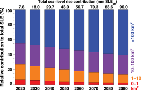
Figure 8. Relative sea-level rise contribution (SLE_eff) of individual glacier size classes averaged over 10-year periods. All results refer to the multi-model mean of RCP4.5.

5.4. ELA/AAR Projections

Regionally averaged glacier ELAs are projected to rise by ~100 to 500 m in the high and mid-latitudes and by ~100 to 800 m in low-latitude regions between 2010 and 2100, depending on the emission scenario (Figure 9). While the ELA change shows a nearly linear rise throughout the projection period for RCP8.5, the rate of ELA rise decreases substantially beyond the middle of the century for RCP4.5 and levels off / reverses for RCP2.6. At the same time accumulation area ratios (AARs) show a tendency to increase for the latter two scenarios, indicating that many glaciers approach a new equilibrium during that period. For RCP8.5, steadily increasing ELAs and AARs dropping below 20% for all regions result in a strong imbalance of the remaining glaciers and, hence, large committed mass losses (Figure 9).

FIGURE 9

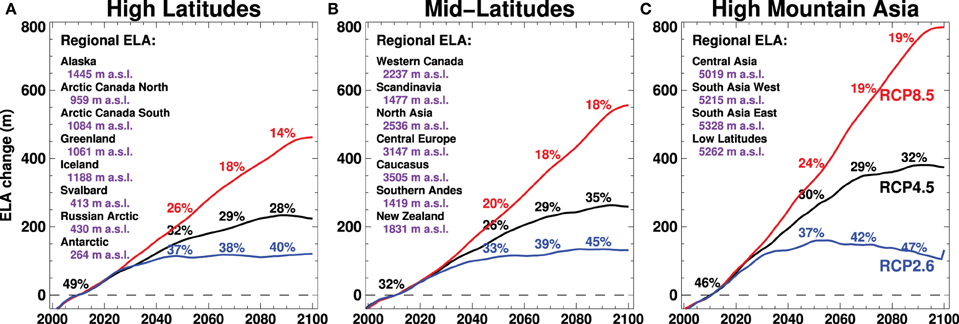
Figure 9. Changes in regional equilibrium line altitudes (ELAs) relative to 2010 for (A) high, (B) mid-, and (C) low latitudes and three emission scenarios. Accumulation area ratios (in %) are given as 20-year averages around 2010, 2050, 2070, and 2090. All values after 2010 are multi-model means. ELAs and AARs are averaged (weighted by glacier area) over all glaciers in the RGI regions listed in each panel. Average ELAs are given for each region for the year 2010.

5.5. Mass Balance Components

Resolving the components of mass loss is important for understanding the drivers of glacier change. Between 1980 and 2000 we find a mean global accumulation rate (snow accumulation plus refreezing) of 803 Gt a⁻¹ (1.10 m w.e. a⁻¹) and an ablation rate (melt plus frontal ablation) of –882 Gt a⁻¹ (–1.21 m w.e. a⁻¹) (Figure 10). Frontal ablation accounts for 10% of total ablation indicating that mass loss is clearly dominated by surface melt. Modeled refreezing represents 3.6% of total accumulation. 91% of ablation is compensated by accumulation suggesting a relatively small imbalance during that period.

FIGURE 10

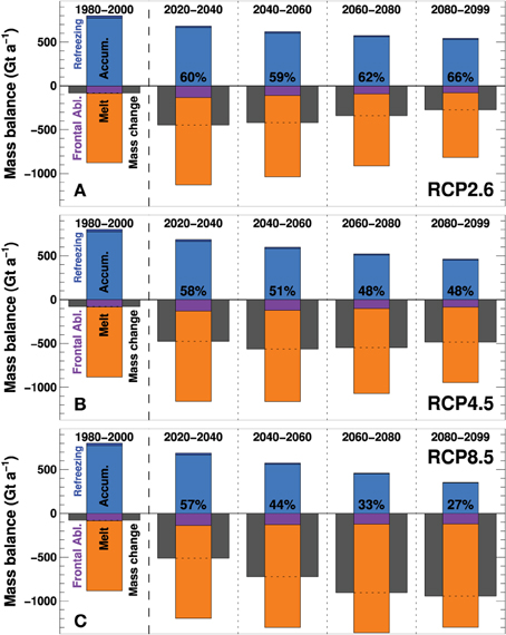
Figure 10. Modeled components of the global glacier mass budget for (A) RCP2.6, (B) RCP4.5, and (C) RCP8.5. Bars show 20-year averages of accumulation, refreezing, melt, frontal ablation, and mass change rates (dark gray). Future periods show multi-model means of all GCMs. Percentages refer to the fraction of ablation that is compensated by mass gain.

For all emission scenarios accumulation rates decrease throughout the century largely due to declining glacier areas (Figure 10). Melt rates increase between the periods 1980–2000 and 2020–2040 but then decrease for RCP2.6 and RCP4.5. Projections driven by RCP8.5 show steadily increasing melt rates until 2060–2080. Also frontal ablation rates increase over the next decades but then are gradually reduced as marine-terminating glaciers retreat onto land (Supplementary Table 8). The differences in frontal ablation rates among the emission scenarios are much less pronounced compared to accumulation or melt rates (Figure 10). The resulting mass imbalances substantially increase at the beginning of the projection period but then change only little for RCP4.5, while being intensified for RCP8.5 despite shrinking glacier areas. For RCP2.6 the net mass change becomes steadily less negative. Refreezing slightly decreases throughout the century (Supplementary Figure 11). By 2030, only 60% of total ablation is compensated by accumulation, irrespective of the emission scenario. Whereas, this fraction stabilizes at around 66% and 48% for RCP2.6 and RCP4.5, respectively, GloGEM indicates a continuously growing imbalance for RCP8.5.

Regional differences in the partitioning of the mass budget and the temporal evolution of its components are illustrated in Figure 11. In contrast to Figure 10, results are shown in specific units, i.e., they are independent of glacier area, and therefore directly comparable in terms of climatic interpretation. All regions show little change in specific accumulation rates despite a tendency of projected precipitation to increase over the twenty-first century (Supplementary Figure 4). Changes in net mass loss are hence largely controlled by the trends in melt rate which greatly vary among the RGI regions. Svalbard and the Russian Arctic show an exceptional acceleration in specific melt rates resulting in highly negative mass balances by the end of the century. In contrast, regions with small initial ice volume (e.g., Central Europe, Low Latitudes) tend toward less negative specific balances indicating that many glaciers have retreated to higher (colder) elevations or have completely disappeared. The Southern Andes are characterized by highest rates of mass turn-over (i.e., maximal accumulation and ablation), and Arctic Canada North by the smallest. The Antarctic and Subantarctic, Svalbard and the Russian Arctic show the largest relative contributions of frontal ablation to total mass loss, reaching >40% by 2030 for glaciers around Antarctica (Supplementary Figure 12). Frontal ablation of individual glaciers shows considerable temporal variations as the snout can either retreat into deeper or more shallow water (Figure 1C). In the regional and global average, some of these effects, however, cancel out.

FIGURE 11

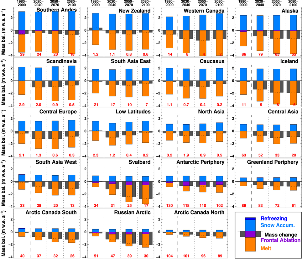
Figure 11. Modeled components of the regional glacier mass budget. Bars show 20-year averages of snow accumulation, refreezing, melt and frontal ablation, and net mass change rates. Future periods show multi-model means of all GCMs forced by RCP4.5. Numbers in red refer to total glacier area in 1000 km². Regions are ordered according to accumulation rates as an indicator of climatic setting (maritime vs continental glaciers).

6. Sensitivity and Uncertainty Analysis

Our results are subject to uncertainties arising from errors in input data, the climate projections, approximations in the model and the calibration procedure. Propagating all potential errors is beyond the scope of this study. Therefore, we perform a comprehensive sensitivity analysis to investigate the most critical uncertainty components. We address the uncertainty due to (i) the choice of the GCM ensemble member, (ii) initial ice volume, (iii) model calibration, and (iv) the type of model formulation to calculate glacier geometry change, frontal ablation and surface melt. Several experiments are performed for each category, and results are compared to those above (henceforth referred to as reference run). Due to computational constraints the experiments are only conducted for four selected regions with different physiographic and climatic settings (Svalbard, Alaska, Central Europe, South Asia West), two GCMs (CanESM2, MPI-ESM-LR) and RCP4.5.

6.1. Choice of GCM Ensemble Member

The large uncertainty in projected glacier wastage due to the choice of the GCM is evident from Figure 6. Here we investigate the impact of using several ensemble runs of the same GCM referring to different equally valid realizations of the GCM with varying initial states of the atmosphere. We run GloGEM with five ensembles for CanESM2 and three for MPI-ESM-LR.

Substantial differences in glacier response among the ensemble members for the same GCMs are found (Figure 12A). The differences from the reference do not show any consistent sign among the regions and the GCMs tested. Whereas, the deviation from the r1i1p1 ensemble run by the end of the century is generally smaller than 10% for Central Europe and South Asia West, two ensembles of MPI-ESM-LR result in almost 40% smaller net mass loss for Alaska. For Svalbard systematically larger net mass losses are predicted for CanESM2 compared to the reference simulation. Although differences may cancel out on a global scale, these results indicate that regional glacier projections can be highly sensitive to the choice of the ensemble member of a GCM.

FIGURE 12

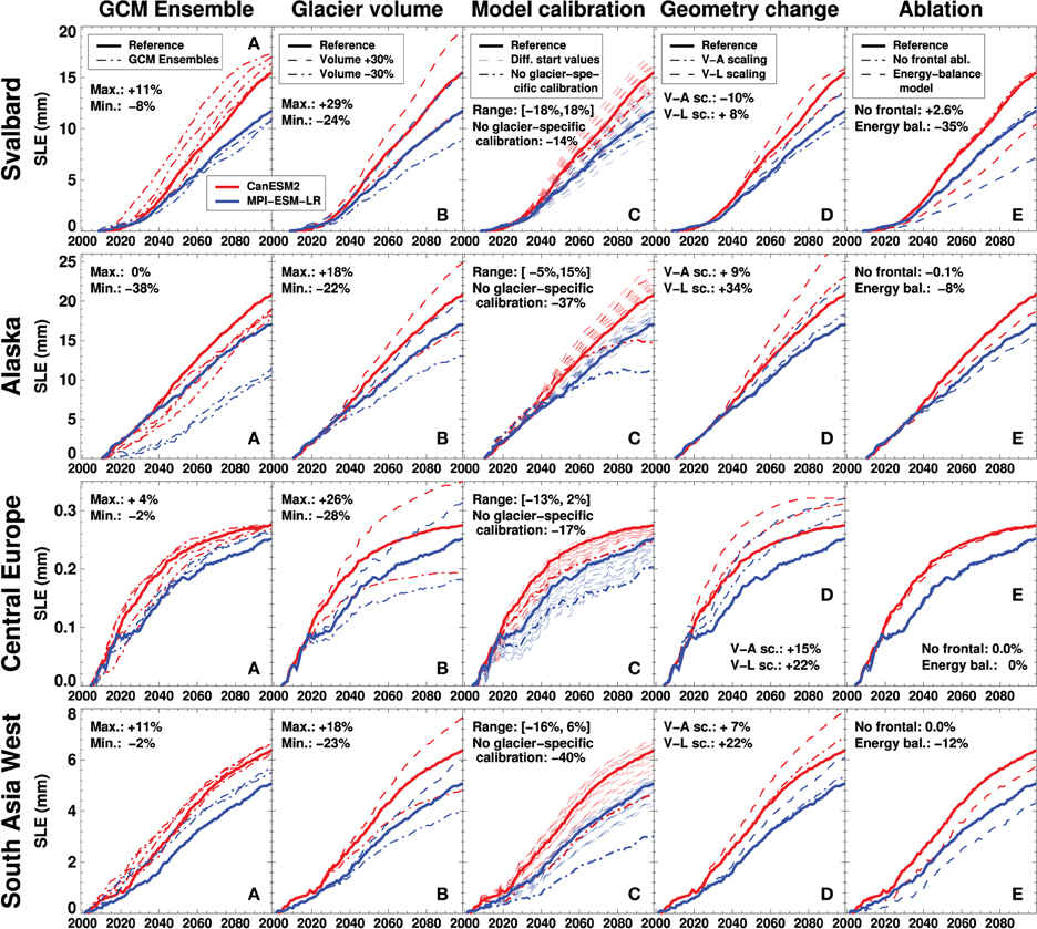
Figure 12. Uncertainty assessment of modeled sea-level equivalent (SLE_ΔM) for Svalbard, Alaska, Central Europe and South Asia West using two GCMs (CanESM2, MPI-ESM-LR) forced by RCP4.5. Sensitivity of SLE to (A) the choice of the GCM ensemble member, (B) variations in initial glacier volume, (C) the technique used to calibrate the model, (D) the approach to calculate glacier geometry change, and (E) the model for frontal ablation and snow/ice melt. Percentages refer to differences between sensitivity experiments and reference runs.

6.2. Initial Ice Thickness

Previous global glacier volume estimates range between ~350 mm and 600 mm SLE (Radić and Hock, 2010; Grinsted, 2013) indicating a large uncertainty in initial ice thickness. We assess the effect of initial ice volume on projected glacier mass change by varying the thickness by ±30% for each glacier and elevation band.

The experiments indicate that calculated glacier mass loss is highly sensitive to initial ice volume (Figure 12B). A 30% increase in initial volume results in 18–29% greater SLE_ΔM by 2100 compared to the reference simulation for the four investigated regions and both GCMs. A volume reduction by the same amount leads to lower SLE_ΔM by roughly the same percentage. Systematic uncertainties in today's ice volume thus translate almost linearly into a bias in calculated sea-level rise contribution.

6.3. Calibration Procedure

We apply two variants of the calibration procedure (Section 4.1): (1) We skip calibration steps 1 and 2, and calibrate the model for step 3 only (Figure 2A). 16 fixed parameter sets based on all combinations of c_prec = [0.8,1.2,1.6,2.0] and f_snow = [1.75,2.7,3.6,4.5] mm d⁻¹ K⁻¹ are prescribed. This approach allows us to estimate the uncertainty arising from choosing initial values for these model parameters. (2) We calibrate the model on the regional mass balance as above but do not force each glacier to agree with this value (Equation 14 instead of Equation 15).

For the former experiment deviations from the reference run are within ±18% (Figure 12C). As the sign of these deviations does not show any consistent pattern among regions, their effect possibly cancels out over a large sample of glaciers and GCMs. In contrast, the impact of calibrating the glacier model only to the regional average mass balance with identical model parameters for each glacier in a region, results in systematically smaller mass losses by –14 to –40% (Figure 12C).

6.4. Modeling Glacier Geometry Change

Previous global projections have relied on volume-area scaling (Slangen et al., 2012; Giesen and Oerlemans, 2013) or volume-length scaling (Marzeion et al., 2012; Radić et al., 2014) to account for glacier retreat or advance. For comparison, we implement both approaches into our model. After calculating an updated glacier ice volume V_t+1 using the mass balance model, a new glacier area A_t+1 is obtained every year as

$\begin{array}{ll}{A}_{t+1}={(V_{t+1}∕c_{\text{A}})}^{(1∕\gamma )},& \left(16\right)\hfill \end{array}$

with γ = 1.375 (1.25) and c_A = 0.0340 (0.0538) km^3−2γ as constants for mountain glaciers (ice caps) (Marzeion et al., 2012). We distribute the area change across all elevation bands by reducing each elevation band's area by the area change in percent relative to the previous year's area. Thus, the area-elevation distribution changes proportionally over the initial elevation range, but glacier length remains unchanged. Analogously, when volume-length scaling is employed, glacier length L_t+1 is calculated as

$\begin{array}{ll}{L}_{t+1}={(V_{t+1}∕c_{\text{L}})}^{(1∕q)},& \left(17\right)\hfill \end{array}$

with q = 2.2 (2.5) and c_L = 0.0180 (0.2252) km^3−q for glaciers (ice caps). This method accounts for the retreat of the glacier to higher elevations but does not include information on the actual ice thickness distribution and, hence, is unable to describe the mass balance-elevation feedback properly. In most experiments, simulated glacier mass loss is higher with the scaling approaches (by 7–34%). Mass loss is larger for length-scaling compared to volume-area scaling for all regions (Figure 12D).

6.5. Neglecting Frontal Ablation

To assess the impact of explicitly modeling mass loss by frontal ablation we disable the corresponding module and re-calibrate the model to regional mass balances according to Figure 2A. The model is then run until 2100 without accounting for frontal ablation.

Excluding frontal ablation has a relatively small impact (0.1–2.5%) on calculated region-wide ice volume change (Figure 12E) although this component accounts for 5–20% of overall ablation for the investigated regions (Alaska, Svalbard). For Svalbard, modeled glacier mass loss even increases if frontal ablation is disregarded. This counterintuitive result can be explained by a compensation of the frontal ablation component with higher surface melt. As our model has been calibrated to match the regional mass change, melt parameters will be higher, corresponding to an increased glacier sensitivity to temperature change.

6.6. Modeling Glacier Melt

Most glacier models operating at the global scale are based on the degree-day approach (e.g., Radić and Hock, 2011; Marzeion et al., 2012). However, several studies have indicated that temperature-index models might be oversensitive to temperature change (Pellicciotti et al., 2005; Gabbi et al., 2014) which would result in an overestimate of future glacier melt. In order to test the sensitivity of global glacier projections to the approach to model snow and ice melt we also implement a simplified energy-balance model into GloGEM and apply it to all regions using all GCMs and emission scenarios.

Energy available for melt E (elevation band i, month m) is computed by

$\begin{array}{ll}{E}_{i,m}=G_{i,m}·(1-{\alpha }_{\text{snow}∕\text{firn}∕\text{ice}})+C_0+C_1·T_{i,m},& \left(18\right)\hfill \end{array}$

where G_{i, m} is the global (i.e., shortwave incoming solar) radiation, α the albedo of snow, firn or ice, C₀ and C₁ are parameters related to the turbulent fluxes and the long-wave radiation balance, and T_{i, m} is the air temperature (Oerlemans, 2001). If E_{i, m} > 0, the melt energy is converted to melt a_{i, m} using the latent heat of fusion. G_{i, m} is calculated by

$\begin{array}{ll}{G}_{i,m}=(\overline{G_{\text{ERA},m}}∕I_{\text{hor},m})·I_{i,m},& \left(19\right)\hfill \end{array}$

where I_{i, m} is the potential clear-sky solar radiation at the glacier surface obtained from solar geometry and each elevation band's aspect and slope (Hock, 1999), $\overline{G_{\text{ERA},m}}$ is ERA-interim global radiation averaged for each month over the period 1980–2010, and I_{hor, m} is the monthly potential solar radiation at the same grid cell assuming a flat surface. Note that I_{hor, m} does not change from year to year. The ratio $(\overline{G_{\text{ERA},m}}∕I_{\text{hor},m})$ accounts for site-specific variations in cloudiness over the year. We apply the same 12 monthly values also for future projections due to the large uncertainties in the GCMs to realistically predict changes in cloudiness (Williams and Tselioudis, 2007).

We calibrate the model for each region according to the approach described above (Figure 2A). Instead of f_snow we tune the parameter C₁ (Equation 18). Validation against direct mass balance measurements indicated a slightly higher RMSE than obtained for the degree-day model, especially regarding the elevation distribution of mass balance (Supplementary Figure 13, Supplementary Table 10). Hence, we do not find an increase in model performance with the more physical approach.

Depending on the emission scenario, calculated SLE_eff is (Supplementary Table 11) reduced by 16–22% (multi-model means of the three RCPs) for the energy-balance model in comparison to the degree-day model (Table 3). The relative reduction is largest for RCP8.5 and smallest for RCP2.6. The most important differences are found for high-latitude regions.

TABLE 3

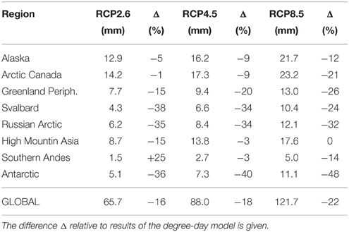
Table 3. Regional estimates of SLE_eff by 2100 for selected regions calculated with the energy balance model.

7. Discussion

7.1. Comparison to Previous Global Estimates

Four independent studies included in IPCC (2013) have calculated global glacier contribution to twenty-first century sea-level rise. Results are directly comparable to ours as (in most cases) the same climate models and glacier inventory data were used. Differences can thus be attributed to model structure and calibration procedures.

Compared to the sea-level rise estimates from glacier wastage reported in the three studies using the same emission scenarios (Marzeion et al., 2012; Slangen et al., 2012; Radić et al., 2014), our multi-model mean estimates of twenty-first century SLE_eff are 15–38% smaller for identical RCPs (Figure 13). Relative reductions are largest for RCP2.6 and smallest for RCP8.5. We note that the uncertainty ranges of all studies overlap. However, our results are systematically lower, also when the results of the various studies are compared for individual GCMs rather than just the multi-model mean.

FIGURE 13

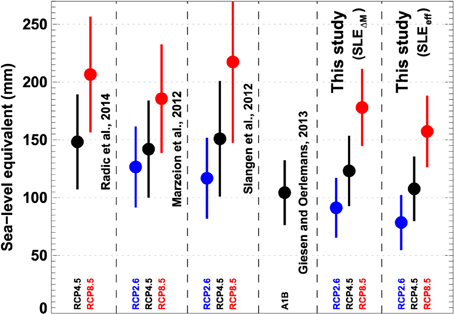
Figure 13. Comparison of modeled twenty-first century sea-level equivalent from glacier mass loss based on previous assessments included in IPCC (2013) with results from this study. Circles refer to multi-model means from 8 to 15 GCMs and bars indicate ±1σ. Previous results are recomputed to refer to the period 2010–2100 -by assuming their average rates to be constant in time. Results of this study are given both as SLE_ΔM and SLE_eff while the results from previous studies denote SLE_ΔM.

In contrast to earlier assessments (which represent SLE_ΔM), we account for ice volume presently below sea level not contributing to sea-level rise when melted. This effect explains about one third of the disagreement. The remainder may be attributed to different calibration procedures and model physics, for example, the description of glacier geometry change. Our sensitivity experiments indicated that volume-area-length scaling generally results in larger glacier net mass loss compared to our approach (Figure 12D), thus providing a possible explanation for our generally lower estimates. We find similar sea-level rise contributions as Giesen and Oerlemans (2013) although results are difficult to compare due to different emission scenarios (Figure 13).

7.2. Model Performance

Model validation indicated a generally good performance of GloGEM for the period 1980–2012 (Section 4.2). Here, we compare our future projections to other studies in the literature that have calculated twenty-first century glacier change for individual glaciers or regions using more sophisticated coupled models for surface mass balance and ice dynamics.

Jouvet et al. (2011) calculated the evolution of Great Aletschgletscher (80 km²), European Alps, using a higher-order ice flow model and regional climate scenarios. Their ice volume change of −88% for 1999–2100 compares well to −80% found with our model (multi-model mean, RCP4.5). For BaltoroGlacier (600 km²), Karakoram, Immerzeel et al. (2012) projected a volume change of −88% over the twenty-first century based on a coupled mass-balance ice-flow model compared to ∓64% from our model. Clarke et al. (2015) found a region-wide volume change of −70% for Western Canada (26,700 km² glacier area) using a physics-based model for ice dynamics driven with a surface mass balance model. For the same domain and GCMs our model yields a similar volume change of −78%. For the Greenland Periphery (90,000 km²) Machguth et al. (2013) projected mass losses of 2000–3900 Gt between 2000 and 2098 using different regional climate models. They applied an energybalance model coupled to a glacier retreat scheme to subregions and subsequently extrapolated results to all glaciers. For the same period we find a cumulative mass loss of −4560 Gt (multi-model mean, RCP4.5).

Despite a very small sample, and differences in input and climate data, the generally good agreement of our results with those from considerably more sophisticated models provides additional confidence that our simplified global model is able to yield projections within the uncertainty range of more complex approaches both for individual glaciers and regions.

7.3. Model Structure

7.3.1. Frontal Ablation

GloGEM is the first global glacier model that includes a frontal ablation module thus allowing us to partition the mass budget into all relevant components. Results must be considered with caution due to the strongly simplified model formulation. Also, the frontal ablation model is highly sensitive to bed topography close to the terminus, and direct observations are scarce to constrain the derivation of ice thickness according to Huss and Farinotti (2012). We expect large uncertainties especially in the Antarctic and Subantarctic where about half of total modeled frontal ablation occurs. More observations of ice thickness are needed to reduce these uncertainties. Nevertheless, our model allows us, for the first time, to approximate the contribution of frontal ablation in global-scale glacier projections.

7.3.2. Adjustment of Geometry

Instead of volume-area or length scaling, as generally used in past global glacier projections, we developed a model that is able to simulate retreat and advance, and annually adjusts glacier surface geometry according to typically observed elevation change patterns. Thus, the model accounts for the mass-balance elevation feedback over the entire glacier. However, just as for the scaling methods, the approach prescribes an immediate geometric response. The model also assumes no elevation change at the highest band, and therefore is not able to fully account for the feedbacks of an ice cap or icefield that experiences progressive thinning at the top (e.g., Trüssel et al., 2015).

7.3.3. Refreezing

In contrast to previous studies relying on simple empirical relations, GloGEM computes refreezing based on modeled temperature profiles. The model does not account for the full range of processes involved but it allows us to approximate the spatio-temporal evolution of refreezing in various climatic settings.

7.3.4. Melt Model

The simplified energy-balance model (Oerlemans, 2001) did not perform better than the simple degree-day model when validated against all available mass-balance observations. This may indicate that energy fluxes other than the short-wave radiation balance may not be represented properly by the formulation that lumps these fluxes into a simple linear temperature dependence. In addition, errors in the global radiation input data and our assumption of constant monthly cloudiness may contribute to reduced model performance.

7.3.5. Calibration Procedure

In the absence of mass-balance observations for all individual glaciers we tune each single glacier of every primary RGI region so that the mean region-wide specific balance rate over the calibration period is reproduced (Equation 15) rather than deriving a uniform set of parameters for each (sub)region (Equation 14) as done in previous studies. Our approach thus assumes each glacier within the same region to have the same average specific mass balance over the calibration period, which is clearly unrealistic. However, the latter approach (Equation 14) leads to unrealistically high spatial variability (Figure 2B) and extremely rapid retreat or advance of individual glaciers due to non-linear effects between surface mass balance and glacier geometry change. Hence, both approaches are not ideal, either over- or underestimating the spatial variability of glacier-wide balance rates within a region. In the optimal case, each glacier was calibrated to observations, however, such data are currently not available at the global scale. While neglecting spatial variability, our approach guarantees that none of the glaciers has specific balance rates beyond plausible limits. In our sensitivity experiment we find that in some regions the alternative approach (Equation 14) leads to substantially less glacier net mass loss by 2100 (Figure 12C). In addition, modeled interannual variability of glacier-wide mass balance (as expressed by the standard deviation) is within 1% of observed variability, if our approach (Equation 15) is adopted, but it is overestimated by about 20% with Equation (14). Both findings indicate possible unrealistic behavior of a considerable portion of glaciers for the latter case including rapid advances and mass gains in response to non-linear feedback mechanisms. As the coverage of geodetic balances will increase, our approach can be refined by tuning parameters for individual subregions or individual glaciers rather than entire primary RGI regions thus accounting for subregion-scale mass balance variability.

Our three-step calibration procedure (Figure 2A) implies that the final parameter set is not unique as it relies on a priori choices of some parameter values. However, exploring the entire parameter space for all glaciers is impossible due to computational constraints. In order to investigate the effect of our calibration procedure on the final calibrated parameter set, we performed a systematic grid search of all parameter combinations within plausible ranges but with relatively large increments (refer to sensitivity experiment in Section 6.3). The resulting future projections scattered randomly around those based on our reference calibration and did not diverge by more than 18% of total mass loss (Figure 12C). For a region with comprehensive direct mass balance observations (Central Europe) we also evaluated the model performance of all alternative parameter combinations for the validation period. We found that our reference parameter set (following the strategy in Figure 2A) performed better than all other tested parameter combinations with respect to root-mean-square error, bias and correlation coefficient for glacier-wide annual and seasonal balance, as well as seasonal mass balance distribution with elevation.

7.4. Regional Differences in Mass Change

Differences in the mass-balance response to twenty-first century climate change among the individual regions are considerable (Figure 6A). In some regions the rate of specific net mass loss steadily increases, whereas, in other regions it stabilizes or the negative trend is even reversed (Figure 11). These variations can largely be explained by differences in initial surface hypsometry which make the glaciers more or less susceptible to similar changes in ELA. The area-elevation distribution controls whether a glacier is able to stabilize by retreating to higher elevations, or is doomed to disappear as the equilibrium line rises in response to a warming climate (Figure 14). For example, in Svalbard and Central Europe, the ELA is projected to rise above the elevations where most initial glacier area is located, and the AAR drops, resulting in a strong imbalance. For Alaska and High Mountain Asia, in contrast, a large fraction of total area remains above the rising ELA. Consequently, glaciers are more likely to reach a new equilibrium.

FIGURE 14

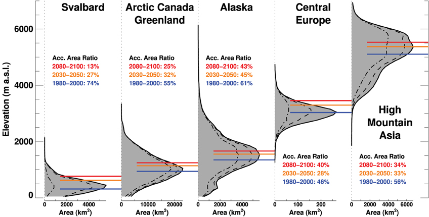
Figure 14. Glacier hypsometry (in 100 m elevation bins) for selected regions at present (shaded), and modeled for 2050 (dashed) and 2100 (dash-dotted) using CNRM-CM5 forced by RCP4.5. The ELA is indicated with solid lines and the corresponding accumulation area ratio is given as a mean for three 20-year periods. ELAs and AARs are area-weighted averages over all glaciers per region.

8. Conclusions

We developed a novel model (GloGEM) for calculating the twenty-first century response of all 200,000 glaciers on Earth outside the ice sheets. The model is forced by monthly temperature and precipitation from 14 GCMs and three emission scenarios. In contrast to previous global-scale glacier models, GloGEM includes mass loss due to frontal ablation of marine-terminating glaciers. Instead of volume-area-length scaling we use an approach that allows glaciers to retreat and advance while also adjusting the surface elevation across the entire glacier. For the first time, we account for the effect of grounded ice below sea level when converting net mass loss to sea-level equivalent. We find a sea-level contribution (multi-model means from 14 GCMs ±1 standard deviation) of SLE_eff of 79±24 mm (RCP2.6), 108±28 mm (RCP4.5) and 157±31 mm (RCP8.5) between 2010 and 2100 which is somewhat lower than found in previous studies. Corresponding volume changes are –25±7%, –33±8%, and –48±9%.

The high-latitude regions (>60°N/S) are the dominant contributors (~78% of total SLE). Sea-level contributions from mid- and low-latitude regions are small or negligible although those regions lose a larger fraction of their current volume by 2100 (>90% for some scenarios and regions). This may have major implications for local and regional water availability. The global glacier mass budget is dominated by snow accumulation and melt; refreezing is a minor component in all regions. Mass losses by frontal ablation of marine-terminating glaciers account for roughly 10% of total ablation globally indicating that this component should be accounted for, although melt clearly dominates ablation in all regions. We find that the glacier contribution to sea-level rise is reduced by about 10% when accounting for the effect of glacier ice grounded below sea level that does not contribute to sea-level rise since it already displaces ocean water.

Calculating snow and ice melt with a simplified energy-balance model instead of a degree-day model yields 16–22% lower estimates of glacier mass loss indicating a smaller sensitivity to temperature change. Despite a more physical approach, model performance slightly decreased in comparison to a classical degree-day model. More research is required to explore ways to implement more physically-based melt formulations into global-scale glacier models.

Consistent with previous studies the diverging climate scenarios among the GCMs cause large uncertainties in our projections. In Svalbard, the range of mass change ranges from negligible to 90% volume loss by 2100 for the same emission scenario. Our sensitivity experiments indicate that the initial ice volume and the model calibration are major sources of uncertainty. More ice thickness data and (sub)regional-scale mass-balance observations are needed to reduce these uncertainties. Nevertheless, the model allows us to approximate possible responses of the world's glaciers to future climate change.

Author Contributions

MH gathered and prepared all data, performed all calculations, and made all figures. He developed the model and modeling procedure with input from RH. MH and RH contributed to the discussion of results, and shared the writing of the paper.

Funding

RH received funding from NASA grants NNX11AO23G and NNX11AF41G.

Conflict of Interest Statement

The authors declare that the research was conducted in the absence of any commercial or financial relationships that could be construed as a potential conflict of interest.

Acknowledgments

This study would not have been possible without several publicly available data sets. We acknowledge the RGI consortium for providing global glacier inventory data, CMIP5 for GCM scenarios, and the ECMWF for the ERA-interim re-analysis data. We thank the World Glacier Monitoring Service and G. Cogley for mass balance data. MH developed part of the code during a month-long visit at the Geophysical Institute of the University of Alaska, Fairbanks.

Supplementary Material

The Supplementary Material for this article can be found online at: https://www.frontiersin.org/article/10.3389/feart.2015.00054

References

Allen, C., Leuschen, C., Gogineni, P., Rodriguez-Morales, F., and Paden, J. (2010/2015). IceBridge MCoRDS L2 Ice Thickness. Boulder, CO: NASA National Snow Ice Data Center Distributed Active Archive Center. doi: 10.5067/GDQ0CUCVTE2Q

CrossRef Full Text

Arendt, A., Bliss, A., Bolch, T., Cogley, J., Gardner, A., Hagen, J.-O., et al. (2014). Randolph Glacier Inventory Ű- A Dataset of Global Glacier Outlines: Version 4.0, Boulder, CO: Digital Media.

Arendt, A. A., Echelmeyer, K. A., Harrison, W. D., Lingle, C. S., and Valentine, V. B. (2002). Rapid wastage of Alaska Glaciers and their contribution to rising sea level. Science 297, 382–386. doi: 10.1126/science.1072497

PubMed Abstract | CrossRef Full Text | Google Scholar

Bahr, D. B., and Radić, V. (2012). Significant contribution to total mass from very small glaciers. Cryosphere 6, 763–770. doi: 10.5194/tc-6-763-2012

CrossRef Full Text | Google Scholar

Benn, D., and Lehmkuhl, F. (2000). Mass balance and equilibrium-line altitudes of glaciers in high-mountain environments. Q. Int. 65, 15–29. doi: 10.1016/S1040-6182(99)00034-8

CrossRef Full Text | Google Scholar

Błaszczyk, M., Jania, J., and Hagen, J.-O. (2009). Tidewater glaciers of Svalbard: recent changes and estimates of calving fluxes. Polish Polar Res. 30, 85–142.

Google Scholar

Bliss, A., Hock, R., and Radić, V. (2014). Global response of glacier runoff to twenty-first century climate change. J. Geophys. Res. 119, 717–730. doi: 10.1002/2013JF002931

CrossRef Full Text | Google Scholar

Braithwaite, R. J. (2008). Temperature and precipitation climate at the equilibrium-line altitude of glaciers expressed by the degree-day factor for melting snow. J. Glaciol. 54, 437–444. doi: 10.3189/002214308785836968

CrossRef Full Text | Google Scholar

Clarke, G. K. C., Jarosch, A. H., Anslow, F. S., Radić, V., and Menounos, B. (2015). Projected deglaciation of western Canada in the twenty-first century. Nat. Geosci. 8, 372–377. doi: 10.1038/ngeo2407

CrossRef Full Text | Google Scholar

Cogley, J. G. (2009). Geodetic and direct mass balance measurements: comparison and joint analysis. Ann. Glaciol. 50, 96–100. doi: 10.3189/172756409787769744

CrossRef Full Text | Google Scholar

Cogley, J. G., Hock, R., Rasmussen, L. A., Arendt, A. A., Bauder, A., Braithwaite, R. J., et al. (2011). Glossary of Glacier Mass Balance and Related Terms, IHP-VII Technical Documents in Hydrology No. 86. Paris: UNESCO-IHP. IACS Contribution No. 2.

Das, I., Hock, R., Berthier, E., and Lingle, C. S. (2014). 21st-century increase in glacier mass loss in the Wrangell Mountains, Alaska, USA, from airborne laser altimetry and satellite stereo imagery. J. Glaciol. 60, 283–293. doi: 10.3189/2014JoG13J119

CrossRef Full Text | Google Scholar

Dee, D. P., Uppala, S. M., Simmons, A. J., Berrisford, P., Poli, P., Kobayashi, S., et al. (2011). The ERA-Interim reanalysis: configuration and performance of the data assimilation system. Q. J. R. Meteorol. Soc. 137, 553–597. doi: 10.1002/qj.828

CrossRef Full Text | Google Scholar

Farinotti, D. (2013). On the effect of short-term climate variability on mountain glaciers: insights from a case study. J. Glaciol. 59, 992–1006. doi: 10.3189/2013JoG13J080

CrossRef Full Text | Google Scholar

Fischer, M., Huss, M., and Hoelzle, M. (2015). Surface elevation and mass changes of all Swiss glaciers 1980–2010. Cryosphere 9, 525–540. doi: 10.5194/tc-9-525-2015

CrossRef Full Text | Google Scholar

Gabbi, J., Carenzo, M., Pellicciotti, F., Bauder, A., and Funk, M. (2014). A comparison of empirical and physically based glacier surface melt models for long-term simulations of glacier response. J. Glaciol. 60, 1140–1154. doi: 10.3189/2014JoG14J011

CrossRef Full Text | Google Scholar

Gardner, A. S., Moholdt, G., Cogley, J. G., Wouters, B., Arendt, A. A., Wahr, J., et al. (2013). A reconciled estimate of glacier contributions to sea level rise: 2003 to 2009. Science 340, 852–857. doi: 10.1126/science.1234532

PubMed Abstract | CrossRef Full Text | Google Scholar

Gardner, A. S., Moholdt, G., Wouters, B., Wolken, G. J., Burgess, D. O., Sharp, M. J., et al. (2011). Sharply increased mass loss from glaciers and ice caps in the Canadian Arctic Archipelago. Nature 473, 357–360. doi: 10.1038/nature10089

PubMed Abstract | CrossRef Full Text | Google Scholar

Gärtner-Roer, I., Naegeli, K., Huss, M., Knecht, T., Machguth, H., and Zemp, M. (2014). A database of worldwide glacier thickness observations. Global Planet. Change 122, 330–344. doi: 10.1016/j.gloplacha.2014.09.003

CrossRef Full Text | Google Scholar

Giesen, R. H., and Oerlemans, J. (2013). Climate-model induced differences in the 21st century global and regional glacier contributions to sea-level rise. Clim. Dyn. 41, 3283–3300. doi: 10.1007/s00382-013-1743-7

CrossRef Full Text | Google Scholar

Glazovsky, A., and Macheret, Y. (2006). “Eurasian arctic,” in Glaciation in North and Central Eurasia in Present Time, ed V. M. Kotlyakov (Moscow: Nauka), 97–114.

Grinsted, A. (2013). An estimate of global glacier volume. Cryosphere 7, 141–151. doi: 10.5194/tc-7-141-2013

CrossRef Full Text | Google Scholar

Haeberli, W., and Linsbauer, A. (2013). Brief communication ”Global glacier volumes and sea level - small but systematic effects of ice below the surface of the ocean and of new local lakes on land”. Cryosphere 7, 817–821. doi: 10.5194/tc-7-817-2013

CrossRef Full Text | Google Scholar

Hirabayashi, Y., Zang, Y., Watanabe, S., Koirala, S., and Kanae, S. (2013). Projection of glacier mass changes under a high-emission climate scenario using the global glacier model HYOGA2. Hydrol. Res. Lett. 7, 6–11. doi: 10.3178/hrl.7.6

CrossRef Full Text | Google Scholar

Hock, R. (1999). A distributed temperature-index ice- and snowmelt model including potential direct solar radiation. J. Glaciol. 45, 101–111.

Google Scholar

Hock, R. (2003). Temperature index melt modelling in mountain areas. J. Hydrol. 282, 104–115. doi: 10.1016/S0022-1694(03)00257-9

CrossRef Full Text | Google Scholar

Howat, I. M., Negrete, A., and Smith, B. E. (2014). The Greenland Ice Mapping Project (GIMP) land classification and surface elevation datasets. Cryosphere 8, 1509–1518. doi: 10.5194/tc-8-1509-2014

CrossRef Full Text | Google Scholar

Huss, M., and Farinotti, D. (2012). Distributed ice thickness and volume of all glaciers around the globe. J. Geophys. Res. 117:F04010. doi: 10.1029/2012JF002523

CrossRef Full Text | Google Scholar

Huss, M., Hock, R., Bauder, A., and Funk, M. (2012). Conventional versus reference-surface mass balance. J. Glaciol. 58, 278–286. doi: 10.3189/2012JoG11J216

CrossRef Full Text | Google Scholar

Huss, M., Jouvet, G., Farinotti, D., and Bauder, A. (2010). Future high-mountain hydrology: a new parameterization of glacier retreat. Hydrol. Earth Syst. Sci. 14, 815–829. doi: 10.5194/hess-14-815-2010

CrossRef Full Text | Google Scholar

Immerzeel, W., Beek, L., Konz, M., Shrestha, A., and Bierkens, M. (2012). Hydrological response to climate change in a glacierized catchment in the Himalayas. Clim. Change 110, 721–736. doi: 10.1007/s10584-011-0143-4

PubMed Abstract | CrossRef Full Text | Google Scholar

IPCC (2013). Climate Change 2013. The Pysical Science Basis. Working Group I Contribution to the Fifth Assessment Report of the Intergovernmental Panel on Climate Change. Technical Report, WMO/UNEP. Cambridge University Press.

Jarvis, J., Reuter, H., Nelson, A., and Guevara, E. (2008). Hole-filled SRTM for the Globe Version 4, Available from the CGIAR-CSI SRTM 90 m Database.

Jóhannesson, T., Raymond, C., and Waddington, E. (1989). Time-scale for adjustment of glaciers to changes in mass balance. J. Glaciol. 35, 355–369.

Google Scholar

Jouvet, G., Huss, M., Funk, M., and Blatter, H. (2011). Modelling the retreat of Grosser Aletschgletscher, Switzerland, in a changing climate. J. Glaciol. 57, 1033–1045. doi: 10.3189/002214311798843359

CrossRef Full Text | Google Scholar

Kaser, G., Cogley, J. G., Dyurgerov, M. B., Meier, M. F., and Ohmura, A. (2006). Mass balance of glaciers and ice caps: consensus estimates for 1961-2004. Geophys. Res. Lett. 33:L19501. doi: 10.1029/2006GL027511

CrossRef Full Text | Google Scholar

Liu, H., Jezek, K. C., Li, B., and Zhao, Z. (2001). RADARSAT Antarctic Mapping Project Digital Elevation Model. Boulder, CO: National Snow and Ice Data Center (National Snow and Ice Data Center, Digital Media).

Google Scholar

Machguth, H., Eisen, O., Paul, F., and Hoelzle, M. (2006). Strong spatial variability of snow accumulation observed with helicopter-borne GPR on two adjacent Alpine glaciers. Geophys. Res. Lett. 33:13503. doi: 10.1029/2006GL026576

CrossRef Full Text | Google Scholar

Machguth, H., Rastner, P., Bolch, T., Mölg, N., Sandberg Sørensen, L., et al. (2013). The future sea-level rise contribution of Greenland's glaciers and ice caps. Environ. Res. Lett. 8:025005. doi: 10.1088/17489326/8/2/025005

CrossRef Full Text | Google Scholar

Marzeion, B., Jarosch, A. H., and Gregory, J. M. (2014). Feedbacks and mechanisms affecting the global sensitivity of glaciers to climate change. Cryosphere 8, 59–71. doi: 10.5194/tc-8-59-2014

CrossRef Full Text | Google Scholar

Marzeion, B., Jarosch, A. H., and Hofer, M. (2012). Past and future sea-level change from the surface mass balance of glaciers. Cryosphere 6, 1295–1322. doi: 10.5194/tc-6-1295-2012

CrossRef Full Text | Google Scholar

McNabb, R. W., Hock, R., and Huss, M. (2015). Variations in Alaska tidewater glacier frontal ablation, 1985–2013. J. Geophys. Res. 120, 120–136. doi: 10.1002/2014JF003276

CrossRef Full Text | Google Scholar

Meier, M. F., Dyurgerov, M. B., Rick, U. K., O'Neel, S., Pfeffer, W. T., Anderson, R. S., et al. (2007). Glaciers dominate Eustatic Sea-Level Rise in the 21st century. Science 317, 1064–1067. doi: 10.1126/science.1143906

PubMed Abstract | CrossRef Full Text | Google Scholar

Meier, M. F., and Post, A. (1987). Fast tidewater glaciers. J. Geophys. Res. Solid Earth 92, 9051–9058. doi: 10.1029/JB092iB09p09051

CrossRef Full Text | Google Scholar

Meinshausen, M., Smith, S. J., Calvin, K., Daniel, J. S., Kainuma, M. L. T., Lamarque, J.-F., et al. (2011). The RCP greenhouse gas concentrations and their extensions from 1765 to 2300. Climat. Change 109, 213–241. doi: 10.1007/s10584-011-0156-z

CrossRef Full Text | Google Scholar

Moholdt, G., Nuth, C., Hagen, J. O., and Kohler, J. (2010). Recent elevation changes of Svalbard glaciers derived from ICESat laser altimetry. Remote Sens. Environ. 114, 2756–2767. doi: 10.1016/j.rse.2010.06.008

CrossRef Full Text | Google Scholar

Moholdt, G., Wouters, B., and Gardner, A. S. (2012). Recent mass changes of glaciers in the Russian High Arctic. Geophys. Res. Lett. 39, 10502. doi: 10.1029/2012GL051466

CrossRef Full Text | Google Scholar

Oerlemans, J. (2001). Glaciers and Climate Change. Rotterdam: A. A. Balkema Publishers.

Google Scholar

Oerlemans, J., Anderson, B., Hubbard, A., Huybrechts, P., Jóhannesson, T., and Knap, W. (1998). Modelling the response of glaciers to climate warming. Clim. Dyn. 14, 267–274. doi: 10.1007/s003820050222

CrossRef Full Text | Google Scholar

Oerlemans, J., and Nick, F. M. (2005). A minimal model of a tidewater glacier. Ann. Glaciol. 42, 1–6. doi: 10.3189/172756405781813023

CrossRef Full Text | Google Scholar

Osmanoglu, B., Braun, M., Hock, R., and Navarro, F. J. (2013). Surface velocity and ice discharge of the ice cap on King George Island, Antarctica. Ann. Glaciol. 54, 111–119. doi: 10.3189/2013AoG63A517

CrossRef Full Text | Google Scholar

Osmanoglu, B., Navarro, F. J., Hock, R., Braun, M., and Corcuera, M. I. (2014). Surface velocity and mass balance of livingston island ice cap, antarctica. Cryosphere 8, 1807–1823. doi: 10.5194/tc-8-1807-2014

CrossRef Full Text | Google Scholar

Pellicciotti, F., Brock, B., Strasser, U., Burlando, P., Funk, M., and Corripio, J. (2005). An enhanced temperature-index glacier melt model including the shortwave radiation balance: development and testing for Haut Glacier d'Arolla, Switzerland. J. Glaciol. 51, 573–587. doi: 10.3189/172756505781829124

CrossRef Full Text | Google Scholar

Pfeffer, W. T., Arendt, A. A., Bliss, A., Bolch, T., Cogley, J. G., Gardner, A. S., et al. (2014). The Randolph Glacier Inventory: a globally complete inventory of glaciers. J. Glaciol. 60, 537–552. doi: 10.3189/2014JoG13J176

CrossRef Full Text | Google Scholar

Pfeffer, W. T., Meier, M. F., and Illangasekare, T. H. (1991). Retention of Greenland runoff by refreezing: implications for projected future sea level change. J. Geophys. Res. 96, 22117. doi: 10.1029/91JC02502

CrossRef Full Text | Google Scholar

Radić, V., Bliss, A., Beedlow, A. C., Hock, R., Miles, E., and Cogley, J. G. (2014). Regional and global projections of twenty-first century glacier mass changes in response to climate scenarios from global climate models. Clim. Dyn. 42, 37–58. doi: 10.1007/s00382-013-1719-7

CrossRef Full Text | Google Scholar

Radić, V., and Hock, R. (2010). Regional and global volumes of glaciers derived from statistical upscaling of glacier inventory data. J. Geophys. Res. 115, 1010. doi: 10.1029/2009JF001373

CrossRef Full Text | Google Scholar

Radić, V., and Hock, R. (2011). Regionally differentiated contribution of mountain glaciers and ice caps to future sea-level rise. Nat. Geosci. 4, 91–94. doi: 10.1038/ngeo1052

CrossRef Full Text | Google Scholar

Radić, V., and Hock, R. (2014). Glaciers in the Earth's Hydrological Cycle: Assessments of glacier mass and runoff changes on global and regional scales. Surv. Geophys. 35, 813–837. doi: 10.1007/s10712-013-9262-y

CrossRef Full Text | Google Scholar

Raper, S. C. B., and Braithwaite, R. J. (2006). Low sea level rise projections from mountain glaciers and icecaps under global warming. Nature 439, 311–313. doi: 10.1038/nature04448

PubMed Abstract | CrossRef Full Text | Google Scholar

Schaefer, M., Machguth, H., Falvey, M., Casassa, G., and Rignot, E. (2015). Quantifying mass balance processes on the southern patagonia icefield. Cryosphere 9, 25–35. doi: 10.5194/tc-9-25-2015

CrossRef Full Text | Google Scholar

Slangen, A. B. A., Katsman, C. A., van de Wal, R. S. W., Vermeersen, L. L. A., and Riva, R. E. M. (2012). Towards regional projections of twenty-first century sea-level change based on IPCC SRES scenarios. Clim. Dynam. 38, 1191–1209. doi: 10.1007/s00382-011-1057-6

CrossRef Full Text | Google Scholar

Tachikawa, T., Hato, M., Kaku, M., and Iwasaki, A. (2011). “Characteristics of ASTER GDEM version 2,” in Geoscience and Remote Sensing Symposium (IGARSS) (Vancouver, BC: IEEE), 3657–3660. doi: 10.1109/igarss.2011.6050017

CrossRef Full Text

Taylor, K. E., Stouffer, R. J., and Meehl, G. A. (2012). An overview of CMIP5 and the experiment design. Bull. Am. Meteorol. Soc. 93, 485–498. doi: 10.1175/BAMS-D-11-00094.1

CrossRef Full Text | Google Scholar

Trüssel, B. L., Truffer, M., Hock, R., Motyka, R. J., Huss, M., and Zhang, J. (2015). Runaway thinning of the low-elevation Yakutat Glacier, Alaska, and its sensitivity to climate change. J. Glaciol. 61, 65–75. doi: 10.3189/2015JoG14J125

CrossRef Full Text | Google Scholar

Van Wychen, W., Burgess, D. O., Gray, L., Copland, L., Sharp, M., Dowdeswell, J. A., et al. (2014). Glacier velocities and dynamic ice discharge from the Queen Elizabeth Islands, Nunavut, Canada. Geophys. Res. Lett. 41, 484–490. doi: 10.1002/2013GL058558

CrossRef Full Text | Google Scholar

WGMS (2012). Fluctuations of Glaciers, 2005–2010, Vol. X. Technical report, ICSU(WDS)/ IUGG(IACS)/ UNEP/UNESCO/ WMO, World Glacier Monitoring Service, Zurich.

Williams, K. D., and Tselioudis, G. (2007). GCM intercomparison of global cloud regimes: present-day evaluation and climate change response. Clim. Dyn. 29, 231–250. doi: 10.1007/s00382-007-0232-2

CrossRef Full Text | Google Scholar