Toward Monitoring Surface and Subsurface Lakes on the Greenland Ice Sheet Using Sentinel-1 SAR and Landsat-8 OLI Imagery

Introduction

The rate of mass loss of the Greenland Ice Sheet (GrIS) has accelerated in recent decades and is increasingly dominated by surface meltwater runoff (Rignot et al., 2011; Vaughan et al., 2013; Csatho et al., 2014; Enderlin et al., 2014). In the ablation and lower accumulation areas, meltwater forms slush zones, supraglacial streams, and supraglacial lakes, which may be located on the surface (surface lakes) or just below it (subsurface lakes). Surface lakes are important as their albedo is lower than that of the surrounding ice, so they enhance energy absorption and meltwater production (Lüthje et al., 2006; Tedesco and Steiner, 2011; Tedesco et al., 2012). They are also significant as they affect the location, timing, volume, and rate of meltwater delivery to the bed, which impacts ice dynamics in different ways depending on whether the lakes drain rapidly, slowly, or do not drain at all and simply freeze at the end of the melt season (Joughin et al., 2013; Selmes et al., 2013; Tedesco et al., 2013).

Rapid lake drainages occur by “hydrofracture” through the ice (Das et al., 2008; Krawczynski et al., 2009; Doyle et al., 2013; Stevens et al., 2015), injecting large water pulses to the bed over a short time period, and substantially enhancing water pressures and ice-sheet movement in the short term (Joughin et al., 2008; Tedesco et al., 2013; Dow et al., 2015; Banwell et al., 2016). Slow lake drainages occur through lake overtopping and the incision of channels by slush removal and ice melt, which may then route water to moulins or crevasses downstream; they deliver smaller water volumes to the bed over longer periods of time, producing moderately high water pressures and increases in ice motion in the short term (Selmes et al., 2013; Tedesco et al., 2013; Dow et al., 2015; Banwell et al., 2016). Lake drainage events are important in opening up moulins, which act as connections between the surface and bed, allowing continued delivery of water through the summer to the subglacial drainage system, facilitating its seasonal evolution and impacting basal water pressures and ice motion over the longer term (Bartholomew et al., 2010; Sole et al., 2013; Tedstone et al., 2013). Increasing amounts of meltwater at higher elevations in the future may allow more lakes to form and drain in those locations, which may lead to an increased hydraulic efficiency of the subglacial drainage system through the formation of channels; however, this is unknown (Mayaud et al., 2014; Leeson et al., 2015).

In addition to their direct effects on ablation and water delivery to the bed, surface lakes are important in the overall water budget of the GrIS as they store water, which may freeze at the end of the summer (Echelmeyer et al., 1991; Rennermalm et al., 2013; Selmes et al., 2013). Subsurface lakes can also store water, although their role in this regard is not well known as they have been observed in just one known previous study, which found lakes containing liquid water through several consecutive winters at an average depth of ~2.0 m below the surface (Koenig et al., 2015).

Previous studies investigating surface lakes have primarily used the optical and infrared wavelengths of MODIS (Box and Ski, 2007; Selmes et al., 2011; Morriss et al., 2013; Fitzpatrick et al., 2014; Williamson et al., 2017), or Landsat (McMillan et al., 2007; Arnold et al., 2014; Banwell et al., 2014; Moussavi et al., 2016; Pope et al., 2016). MODIS has a high temporal resolution (daily) whereas the Landsat satellites have a high spatial resolution [30 m for Landsat-8 Operational Land Imagery (OLI)]. However, both the low spatial resolution of MODIS (250 or 500 m) and low temporal resolution of Landsat-8 OLI (at best a four-day repeat, although frequently up to 16 days) makes them poorly suited to the investigation of small lakes that may change rapidly. Furthermore, such sensors are unable to image through cloud or in darkness, restricting the number of useful scenes that can be used (Selmes et al., 2013; Williamson et al., 2017).

Radar imagery can overcome some of the limitations of optical and infrared imagery as it can detect the Earth's surface under any light or cloud conditions. It also penetrates snow and firn and can therefore be used to identify buried subsurface lakes. Synthetic Aperture Radar (SAR) sensors aboard satellites such as TerraSAR-X and ENVISAT tend to compromise either the temporal resolution or swath coverage, and the application of these sensors to supraglacial hydrological investigations has been limited and not focussed on lake detection (Bindschadler and Vornberger, 1992; Johansson and Brown, 2012; Joughin et al., 2013; Luckman et al., 2014). The airborne Operation IceBridge Snow Radar (~2–6.5 GHz) has detected buried lakes (Koenig et al., 2015) although the limited spatial and temporal coverage of the data restricts the mapping of their area and changes through time.

The Sentinel-1 SAR sensors have the potential to improve the knowledge and understanding of GrIS lakes and their dynamics by overcoming many of the weaknesses of the other sensors. The C-band (~5.4 GHz) SAR can image through clouds. The high spatial resolution (25 or 40 m for high- and medium-resolution, respectively) is comparable to Landsat-8 (30 m) and superior to MODIS (250 or 500 m). The greater temporal resolution (12-day repeat passes for both Sentinel-1A and -1B, giving a combined six-day repeat) compared to Landsat-8 (16-day repeat) enables the filling and draining of small lakes (smaller than can be seen using MODIS) to be detected with high temporal precision. They can image in darkness, allowing the detection of lakes and lake behavior late into the melt season and through the winter. Finally, the radar waves penetrate the surface snow and firn layers, allowing the detection and analysis of subsurface water bodies.

Our study uses Sentinel-1 SAR together with Landsat-8 OLI imagery (hereafter Sentinel-1 and Landsat, respectively) from 2015 to identify the spatial and temporal extent of surface and subsurface lakes across part of the GrIS, and their temporal changes over the summer and into the early winter. The combination of Sentinel-1 and Landsat allows us to mosaic a time series of imagery that is approaching the temporal resolution provided by MODIS imagery alone. It is restricted to using Sentinel-1A SAR only as Sentinel-1B was not launched until 2016. Our main objectives are to:

1. Use Sentinel-1 imagery guided by Landsat imagery to develop a semi-automated lake-classification method, and determine which of the SAR polarizations provides the best approach;

2. Use the lake classification from (1) together with an existing Landsat lake classification method to automatically detect fast and slow surface lake drainage events from all of the available Sentinel-1 and Landsat images.

Our secondary objectives are to:

1. Manually identify surface lake freeze-through from Landsat and Sentinel-1 imagery;

2. Manually detect subsurface lake appearance and freeze-through from Sentinel-1 imagery.

Data and Methods

Study Region

The study region covers ~42,000 km² of West Greenland, which has an extensive and active supraglacial hydrological system, including a high concentration of supraglacial lakes (Lewis and Smith, 2009; Selmes et al., 2011; Figure 1). Previous remote sensing studies in the area have quantified supraglacial lake area and volume (e.g., Box and Ski, 2007; Georgiou et al., 2009; Williamson et al., 2017) and found that lakes have been forming and draining at higher elevations as melt rates have increased in recent years (Selmes et al., 2011; Howat et al., 2013; Fitzpatrick et al., 2014; Pope et al., 2016), particularly in very warm years, when lakes also drain earlier (Liang et al., 2012). The study region was chosen to match the total extent of the selected Landsat-8 scenes (paths 006, 007, 008, 009, and 010, and rows 011 and 012; Figure 1). Although not all of the images always covered the full study region, all scenes were included to give the best possible temporal resolution (Supplementary Tables 1, 2).

FIGURE 1

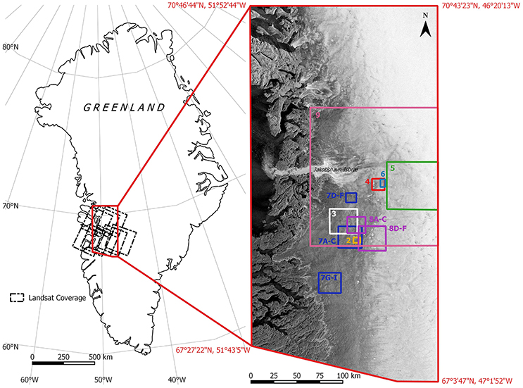
Figure 1. Location of the study region within Greenland, showing the coverage of the Landsat scenes used to define the boundary of the study region. The inset shows the areas used on subsequent figures that do not cover the full study region, mapped onto a Sentinel-1 image (HH polarization) from day 287 (2015).

Pre-processing

Landsat and Sentinel-1 SAR images were acquired between mid-June and late September 2015 to allow for the detection of summer lake extent and drainage. Additional Sentinel-1 images from October to November 2015 were used to extend the analysis beyond the summer. Figure 2 displays the processing steps for summer lake detection, from the acquisition of the raw imagery to the creation of a binary lake mask. A total of 13 atmospherically corrected Landsat surface reflectance images with <10% cloud cover from 20 June to 25 August were downloaded (Figure 2A; Supplementary Table 1). Scenes from the same day were mosaicked, and the bedrock and ocean were cropped using a mask created from the Greenland Ice Mapping Project (GIMP) Digital Elevation Model (DEM) (Howat et al., 2014).

FIGURE 2

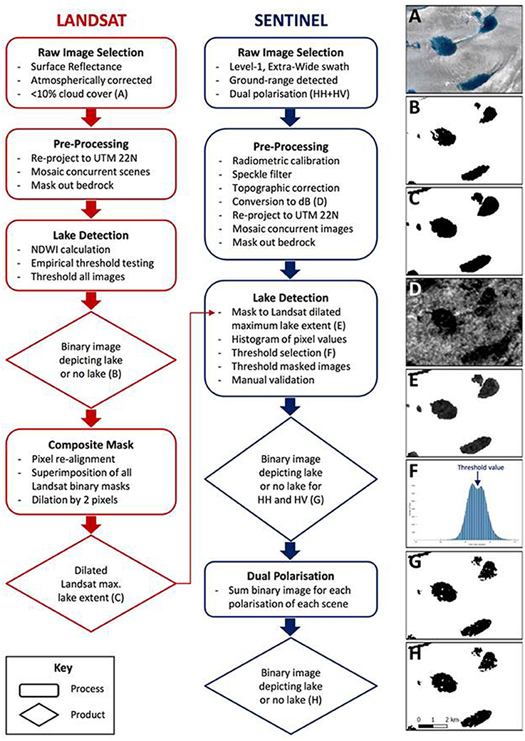
Figure 2. An illustrated flow diagram outlining the methodology followed for both the Landsat and the Sentinel-1 lake detections. Illustrated steps are labeled (A–H) within the diagram and all refer to the same areal extent (shown in Figure 1); the Landsat-8 false-color RGB image in (A) and pre-processed HV polarized image shown in (D) were acquired on day 189 (2015).

Sentinel-1 Level-1 images were used since they are georeferenced but minimally processed. The Extra-Wide swath (400 km with 5 sub-swaths) provided the best coverage without compromising the spatial resolution. At the start of the study period, only medium-resolution images were available due to the recent launch of the satellite, so throughout the summer period the highest possible resolution was selected (Supplementary Table 2). Dual-polarization images (HH and HV) were chosen in the Ground-Range Detected mode. A total of 28 summer images spanning 15 June to 30 September was obtained. We used the Sentinel Application Platform (SNAP) toolbox to carry out a radiometric calibration, a single product speckle filter and a topographical correction on each raw Sentinel-1 scene (Copernicus, 2016). This last process used a Range Doppler terrain correction operator, which corrected the terrain and image orientation using bilinear interpolation of the GETASSE30 DEM. The image backscatter values were converted to decibels (dB) using:

$\begin{array}{cc}Image \left(dB\right)=10 \times \text{log}(image)& (1)\end{array}$

(Figure 2D). The two polarizations (HH and HV) of each image were subsequently treated as separate images, rather than as a single scene with two bands. Concurrent images were mosaicked, and the bedrock and ocean were cropped using the GIMP DEM mask (Howat et al., 2014). For some of the Sentinel-1 scenes acquired on the same day, pre-processing resulted in a gap between the two mosaicked edges; the resultant spaces of under a pixel width between the two images were treated as “no data” values, and accounted for in subsequent processing.

Lake Detection

Surface lakes were detected in the Landsat imagery using the Normalized Difference Water Index (NDWI), a well-established band-math technique that classically uses a ratio involving the red (B4, 0.64–0.67 μm) and blue (B2, 0.45–0.51 μm) bands (Huggel et al., 2002; Xu, 2006; Doyle et al., 2013; Morriss et al., 2013; Yang and Smith, 2013; Moussavi et al., 2016):

$\begin{array}{cc}NDWI= \frac{B_2-B_4}{B_2+B_4}.& (2)\end{array}$

A threshold value of 0.5 was selected empirically as sufficient to define lakes without including surrounding water or slush areas. Sensitivity to this threshold was tested qualitatively by comparison with the original red-green-blue (RGB) false-color images. Higher thresholds produced smaller lake areas, but excluded shallow water that was obviously associated with lakes. Lower thresholds gave larger lake areas but included many pixels that looked like streams or isolated slush patches. The NDWI threshold of 0.5 was applied to all Landsat scenes to create a lake mask for each image (Figure 2B). All of the binary images were then superimposed to create a composite mask of Landsat-derived maximum lake area over the study period. This composite maximum lake area mask was then dilated by two pixels (i.e., 60 m; Figure 2C).

The dilated mask was applied to each Sentinel-1 scene to produce, for each image, the backscatter values of all pixels that either: (i) appear as surface lakes in the Landsat scenes at some stage of the summer; or (ii) immediately surround those pixels (Figure 2E). The histogram of each masked Sentinel-1 image was then examined and, where a bimodal distribution existed between the lower lake backscatter values and the higher surrounding slush or ice backscatter values, the lowest point between the peaks was selected as a backscatter threshold value to define lake area for that particular image (Figure 2F). The two-pixel buffer value was chosen empirically by application to several images. Sensitivity to the buffer value was tested qualitatively by viewing the resultant backscatter histograms. A smaller buffer obscured the bimodal distribution in some images, whereas a larger buffer did not improve the clarity of the bimodal histogram in any image. Applying a buffer was necessary due to slush surrounding some lakes having similar backscatter values to the lakes, thereby complicating the differentiation of slush and water (Bindschadler and Vornberger, 1992). Threshold values were picked manually from each histogram, and varied from −16 to −29 dB for the HH images, and −22 to −29 dB for the HV images (Supplementary Table 2). The masked Sentinel-1 images were thresholded by their unique saddle value to produce binary images akin to the thresholded Landsat images (Figure 2G). Of the original 28 Sentinel-1 images, 23 were suitable for further analysis, since if no bimodal histogram was present, the image was discarded. Finally, for each time period, the binary images of the two polarizations were superimposed to produce a total Sentinel-1-derived lake area (Figure 2H).

Sensitivity to the Sentinel-1 backscatter threshold values was evaluated for three dates during the summer: days 189, 212, and 237. For each image, its unique threshold value was shifted up and down in 1 dB increments to examine the effect of varying thresholds on total lake area (Supplementary Figures 1, 2). For all images, sensitivity is approximately linear over most of the range but the magnitude varies between the images. On day 212, the sensitivity is ~30 km² dB⁻¹; on day 189 and 237, it is approximately five times greater at 150 km² dB⁻¹ (Supplementary Figure 1). Compared to the chosen threshold value (Supplementary Figure 2B), lowering the threshold diminishes the number of pixels designated as lakes, so some lakes appear patchy (Supplementary Figure 2A). Raising the threshold value increases the number of pixels depicted as lakes, with more lakes identified and each covering a larger area up to the full extent of the mask (Supplementary Figures 2C,D).

On the three dates used for the threshold backscatter sensitivity analysis, there were contemporaneous images from both the Sentinel-1 and Landsat sensors with some areal overlap. For these dates, the lake areas detected from each type of imagery within the overlapping regions were compared, forming the basis of our evaluation of the Sentinel-1 classification scheme with respect to the Landsat NDWI technique, and enabling the most suitable Sentinel-1 polarization to be determined.

Lake Drainage

Surface lake drainages were easily distinguished from the Landsat imagery: Figures 3A–C show lakes that either disappear rapidly between two images (red and green circles), or more slowly over several consecutive images (yellow circles). These drainages were also detected in Sentinel-1 imagery. Areas of low backscatter created by lakes in one image change to values that are similar to the surrounding ice once the water has drained (Figures 3D–F, yellow circles). An intermediate stage was observed in some instances, where the low lake backscatter flips to very high backscatter values in the next image, before then changing to values that are similar to the surrounding ice (Figures 3D–F, red and green circles). This succession was also noted by Johansson and Brown (2012) using ENVISAT ASAR. We interpreted this sequence as a lake, then a rough heterogeneous surface consisting of patches of slush and ice left behind after the initial drainage producing the high backscatter values, and then a smoother, more homogeneous ice surface once the water within the slush drains and the snow melts. This sequence did not always feature in the imagery, however, so could not be used to inform our drainage detection.

FIGURE 3

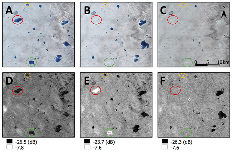
Figure 3. Example surface lake drainage events in Landsat RGB false-color imagery (A–C) and Sentinel-1 HH polarization (D–F); location within the study region is shown in Figure 1. Image (A) was acquired on day 189, (B) on day 196, (C) on day 212, (D) on day 188, (E) on day 190, and (F) on day 200 (all 2015). The yellow circles indicate a “standard” drainage event; the green and red circles highlight two lakes that drain with an intermediate stage observed in the Sentinel-1 imagery.

Our drainage detection methodology was used on three datasets: (i) only Landsat data; (ii) only Sentinel-1 data; and (iii) the combined Landsat–Sentinel-1 dataset, using images from 20 June to 30 September. These three separate analyses allowed us to assess the extra information about lake filling and draining that can be obtained using Sentinel-1 data instead of, or in addition to, Landsat data. Our lake drainage detections were derived using Williamson et al.'s (2017) Fully Automated Supraglacial lake Tracking (FAST) algorithm, which was originally developed for MODIS imagery. The FAST algorithm creates a maximum lake extent array from all available summer lake extents from the relevant imagery, and then tracks changes to the individual lake areas within these maximum extents over the sequence of imagery. For each lake, a rapid drainage event was identified if a lake lost >80% of its area within ≤96 h. Although some rapid lake drainage events are known to occur in under 24 h (Das et al., 2008), this four-day threshold is in line with definitions for rapid drainage events used in previous remote sensing studies: two days (Selmes et al., 2011, 2013); four days (Doyle et al., 2014; Fitzpatrick et al., 2014; Williamson et al., 2017); five days (Liang et al., 2012); and six days (Morriss et al., 2013). Slow drainage events were defined as when a lake lost >20% of its area over any time period, after any previously identified rapidly draining lakes were removed from the dataset.

Lakes >0.25 km in diameter (areas >0.0491 km² when approximated as perfect circles) have been found to hold a sufficient water volume to hydrofracture through subfreezing ice 1–1.5 km thick on the GrIS (Krawczynski et al., 2009). We therefore only track lake areas that reach 55 pixels (0.0495 km²) in size at least once in the season, since we can be confident that these lakes might be able to initiate hydrofracture (Krawczynski et al., 2009). The smallest lake size typically used in MODIS studies is 0.125 km² (i.e., two 250 m pixels) due to its lower spatial resolution (Selmes et al., 2011, 2013; Williamson et al., 2017). Our algorithm differentiates between “large” and “small” lakes to assess the difference in lake behavior by lake size. “Large” lakes are those ≥0.125 km² (i.e., those resolvable in MODIS); “small” lakes are <0.125 km². The “date of drainage” was defined as the midpoint between the dates of the two images over which the lake disappears (following Doyle et al., 2013). We also calculated an associated error on the lake drainage date as half of the number of days between these two images.

Lake Freeze-Through

The Landsat and Sentinel-1 imagery was used further to investigate the behavior of surface lakes at the end of the melt season. In the Landsat imagery, freeze-through was detected manually for each lake when it appeared optically similar to the surrounding ice surface (cf. Johansson et al., 2013; Selmes et al., 2013; Luckman et al., 2014). If a lake had not frozen at the end of the available imagery, a freeze-through date was not recorded. When new snowfall obscured freeze-through detection, the day on which the new snow obscured the lake was recorded. This occurred for lakes at higher elevations due to new snowfall observed on the 16 August.

In the Sentinel-1 imagery, freeze-through was also detected manually for each lake. Areas of low backscatter were apparent in the Sentinel-1 images after 16 August (Figure 4); these are interpreted as liquid water beneath a fresh, dry snow cover that is invisible to microwave wavelengths (König et al., 2001). SAR allows the time of freeze-through to be determined directly, as bubbles entrained within frozen lake ice increase the relative backscatter compared to liquid water (Hirose et al., 2008). The backscatter signal of unfrozen and frozen lakes is therefore sufficiently distinct to allow freeze-through identification (Johansson and Brown, 2012). We defined freeze-through as having occurred once the backscatter values within a lake basin were comparable to those of the surrounding glacial ice, similar to our method for detecting lake drainage. As the C-band penetration depth is limited to a few meters, we recognize that a lake may not have frozen through fully, but may have frozen through only to the depth of the SAR wave penetration.

FIGURE 4

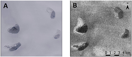
Figure 4. Example of surface lakes partially obscured by snow (location shown in Figure 1) in the Landsat RGB false color image on day 235 (2015) (A), but still detected as liquid water in the Sentinel-1 image (HV polarization) on day 232 (2015) (B).

In both the Landsat and Sentinel-1 imagery, freeze-through events were recorded for lakes that never drained, but also for lakes that partially drained earlier in the melt season; there are therefore lakes that appear in both the drainage and the freeze-through categories. The “date of freeze-through” and associated error were calculated in the same ways as for the lake drainage events defined above.

Subsurface Lakes

Late in the summer, small dark areas appear in the Sentinel-1 imagery at generally higher elevations than the surface lakes discussed so far (Figure 5B). In the Landsat scenes, these are either never visible (Figure 5A, red circles), or appear as large, ice-covered depressions with a small moat of water around their perimeter (Figure 5A, green circles). These areas of water would have been included in the surface lake detection process described in the Lake Detection section above. The dark areas in the Sentinel-1 imagery have similar backscatter values to the snow-covered unfrozen lakes (see Lake Freeze-Through section above), and are interpreted, therefore, as ponded subsurface liquid water. These features were delineated manually from the Sentinel-1 imagery only, as there were no contemporaneous Landsat images that would have allowed a similar detection procedure as for the surface lakes (see Lake Detection section above). The “date of appearance” and “date of disappearance” of each subsurface lake were determined manually as the midpoint between the images before and after the lake first appeared and was last present, respectively. The associated errors in these dates were calculated in the same way as for the surface lake drainages and freeze-through events defined above.

FIGURE 5

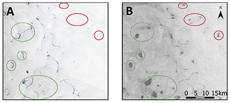
Figure 5. Example of subsurface lakes in a Landsat false-color image (A; day 212, 2015) and a later Sentinel-1 image (B; acquired on day 239, 2015, HH polarization). A later Landsat scene was not available in this location due to cloud cover. The location within the study region is shown in Figure 1. Green circles illustrate subsurface lakes that are partially visible in the Landsat image due to some peripheral melting; red circles demonstrate lakes that are never visible in the Landsat imagery.

Results

Lake Detection

Figure 6 shows the total lake areas detected in each Sentinel-1 image, depicting separately the areas detected by the HH polarization, the HV polarization, and both polarizations. Some of the image-to-image variation in lake area was due to the varying image coverages and to the error in the total lake area (error bars, Figure 6). The HV polarization typically classified a much greater lake area than the HH polarization. Furthermore, pixels classified using the HH polarization were usually also classified by the HV polarization, so the HH polarization generally added few additional lake pixels to the classification based solely on the HV polarization. There were exceptions; the greatest of these was on day 190, where the HH polarization identified more unique lake pixels than the HV polarization.

FIGURE 6

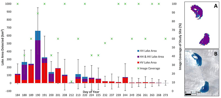
Figure 6. Total lake areas detected by the Sentinel-1 method (bars), colored by the areas classified by the HH polarization (blue), the HV polarization (red), or by both polarizations (purple, i.e., the overlapping region of the red and blue bars). The upper and lower error bars were calculated taking the average root mean square error over all of the images (Table 1) and then multiplying it by the number of lakes on an individual daily image. The area covered by each Sentinel-1 image (as a percentage of the full study region shown in Figure 1) is also plotted (stars) to help interpret the varying lake areas between the days. The insets display two lakes: (A) shows the polarization(s) from which each lake pixel was derived during the Sentinel-1 lake classification method (day 190, 2015); (B) shows the closest available Landsat false-color image (day 196, 2015) for comparison (location within the study region shown in Figure 1).

Table 1 compares the lake areas detected by Sentinel-1 and by Landsat for the three days when there were overlapping images. For each day, the total lake area classified by the Landsat NDWI scheme was closer to the area produced using the Sentinel-1 HV polarization than the HH polarization, with the best match given when the lake areas produced from both the HV and HH polarizations were combined (Table 1). This validates the final stage in our Sentinel-1 lake detection methodology: the use of both the HV and the HH polarization detections in combination for defining lakes from Sentinel-1 imagery (Figure 2H).

TABLE 1

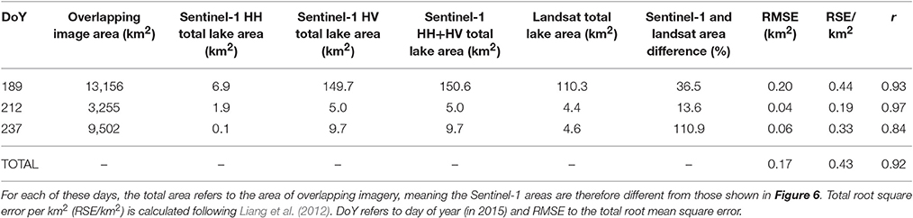
Table 1. Results from the Landsat and Sentinel-1 surface lake detection methods for the three days when there was overlapping imagery.

Examples of the Landsat and Sentinel-1 lake detections on the three days with contemporaneous images are shown in Figure 7. The Sentinel-1-detected lake shapes, sizes and areas were generally similar to those detected in the Landsat scenes: for example, on day 189 (Figures 7A–C) and day 237 (Figures 7G–I). However, the larger lakes depicted by our Sentinel-1 scheme on day 212 were more poorly defined than those detected by Landsat (Figures 7D–F), while the Sentinel-1-derived lakes on day 237 (Figure 7I) showed pixels designated as water that were not shown as water in the Landsat images (Figures 7G,H). Overall, the Sentinel-1 lake detection calculated a greater total lake area than the Landsat NDWI classification within the same region, and the percentage differences between the lake detections varied enormously from 13.6 to 110.9% (Table 1). The total root mean square error (0.17 km²) was comparable to values found in previous studies, but the total root square error per km² (0.43, as defined by Liang et al., 2012) was typically an order of magnitude larger, although the previous studies were comparing two types of optical imagery (Sundal et al., 2009; Selmes et al., 2011; Liang et al., 2012; Williamson et al., 2017). The Pearson's r-value in Table 1 (0.92) shows that the lake areas determined by each method were highly correlated. The mean individual lake areas across all lakes detected from both Landsat and Sentinel-1 images were 0.235 and 0.115 km², respectively.

FIGURE 7

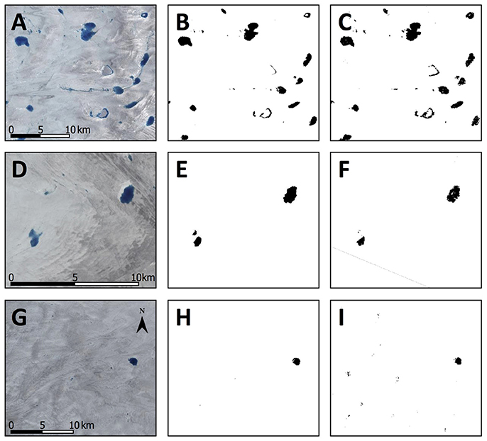
Figure 7. Examples of lake classifications, with Landsat RGB false-color images for reference (A,D,G), classified by the Landsat NDWI (B,E,H) and Sentinel-1 (C,F,I). Locations within the study region are shown in Figure 1. Subsets (A–C) were acquired on day 189 (2015); subsets (D–F) were acquired on day 212 (2015); subsets (G–I) were acquired on day 237 (2015).

An assessment of lake areas with elevation was made as a further component of our Landsat–Sentinel-1 comparison. We found no systematic bias in the lake area detections with respect to elevation for either dataset. Early in the melt season, Sentinel-1 tended to overestimate lake area at higher elevations and marginally underestimate areas at mid-elevations compared to Landsat, although the differences were small.

There were three instances where the Sentinel-1 scheme had difficulty depicting lake areas; examples are shown in Figure 8. First, there were times when lakes were visible in Landsat, appearing, as expected, with low backscatter values in the HV polarization, but appearing with very high backscatter values in the HH polarization (Figures 8A–C). Second, there were times when lakes visible in Landsat were invisible in the HH polarization, but were seen in the HV polarization (Figures 8D–F, red circles). Third, there were times when lakes absent in the Landsat imagery appeared as low backscatter in the Sentinel-1 images, comparable to values representing water, in both the HH and HV polarizations (Figures 8D–F, green circles).

FIGURE 8

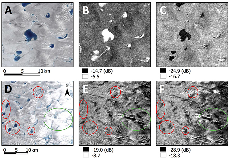
Figure 8. Examples of where the Sentinel-1 lake detection method could not accurately depict lakes; Landsat false-color images are shown from day 196 (2015) (A) and day 189 (2015) (D) for reference, with the Sentinel-1 HH polarization backscatter image (B,E) and the HV polarization image (C,F). Locations within the study region are shown in Figure 1. Subsets (B,C) were imaged on day 201 (2015); (E,F) on day 191 (2015). Subsets (A–C) display lakes that unexpectedly produce very high backscatter values in the HH polarization (B) but typical low backscatter values in the HV polarization (C). Subsets (D–F) display lakes (red circles) that are undetectable in the HH polarization (E) despite being visible in the Landsat (D) and HV polarization (F), as well as areas of very low backscatter (green circles) where no water is visible in the Landsat imagery.

Lake Drainage

The combined Landsat–Sentinel-1 image dataset had a mean temporal resolution of 3.1 days, compared to 4.7 and 8.6 days for the Sentinel-1 and Landsat datasets, respectively. Consequently, the combined image analysis detected a greater number of drainage events with smaller date uncertainties than the single image analyses (Table 2; Supplementary Figure 3). The overall uncertainty in the mean drainage date for the combined Landsat–Sentinel-1 analysis (±4.0 days) was half that for the Landsat analysis (±8.0 days; Table 2). Compared to the Sentinel-1 analysis, the Landsat analysis detected more drainage events (Table 2), despite the smaller number of scenes (12 vs. 22) and the typically smaller coverage of each Landsat mosaic compared to each Sentinel-1 mosaic: the mean area compared to the full study region was 46 vs. 74%, respectively (Supplementary Tables 1, 2). This highlights the potential bias in the single imagery datasets that have a poorer temporal resolution compared to the combined dataset.

TABLE 2

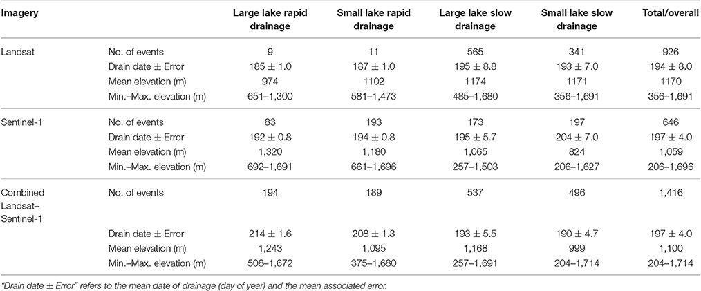
Table 2. Results from the drainage detection algorithm, for the three imagery analyses (Landsat only, Sentinel-1 only, and Landsat–Sentinel-1 combined).

The combined dataset allowed large and small lake areas to be tracked; the mean lake size was 0.089 km². Compared to the total lake population (1,749 lakes), 11% of lakes were large and drained rapidly, 11% were small and drained rapidly, 31% were large and drained slowly, and 28% were small and drained slowly. The mean drainage date from the combined image analysis and the Sentinel-1 analysis alone is 16 July (±4.0 days). The date for the Landsat analysis is slightly earlier (13 July; ±8.0 days) and is affected by the dataset containing fewer images and ending earlier in the season (Table 2, Supplementary Tables 1, 2). The mean drainage date of the combined analysis shows a noticeable difference according to the lake size: compared to large lake drainages, small lake drainages occur an average of six days earlier for rapid drainage events, and three days earlier for slower events (with an overall mean of 4.5 days earlier for both types of event).

The mean elevation of all draining lakes is comparable for the three analyses: 1,100 m for the combined analysis, 1,170 m for the Landsat analysis, and 1,059 m for the Sentinel-1 analysis (Table 2). Overall, drainage tends to occur later in the summer with increasing elevation (Supplementary Figure 3). The combined analysis also shows that small lake drainage events occur at lower elevations than large lake drainages (overall mean 159 m difference). Specifically, small rapid events were observed to occur an average of 148 m lower than large rapid events, and small slow events were 169 m lower than large slow events.

Lake Freeze-Through

A total of 621 lake freeze-through events was identified from the Landsat and Sentinel-1 imagery (Table 3). The Landsat-detected dates (Table 3; Supplementary Figure 4A) have a smaller range and larger errors (Supplementary Figure 4C) than the Sentinel-1-detected dates (Supplementary Figures 4B,D). The mean freeze-through date detected by Sentinel-1 (30 August) is over 2 weeks later than that seen in Landsat (12 August; Table 3). The mean elevation of freezing lakes is ~100 m higher than the mean elevation of lakes that drained (cf. Tables 2, 3), although there is no statistically significant correlation between lake freeze-through date and elevation for either set of imagery (Table 3).

TABLE 3

Table 3. Results from the surface lake freeze-through detections of the Sentinel-1 and the Landsat data. DoY refers to day of year (in 2015).

Subsurface Lakes

The mapped subsurface lakes show a similar distribution and density to the buried lakes identified by Koenig et al. (2015) using IceBridge Ice Sounding Radar (Figure 9). We interpret our subsurface lakes to be similar features to the Icebridge-detected buried lakes. There are differences between the two datasets, which is to be expected as the data were acquired in different years. Koenig et al. (2015) note that buried lakes often appear in particular locations for just a single year, though can recur, and they map buried lakes for 2009, 2010, and 2012 (Figure 9A). In contrast, the subsurface lakes mapped in this study are from 2015 only (Figure 9B).

FIGURE 9

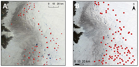
Figure 9. Comparison of the buried lake distribution mapped by Koenig et al. (2015, their Figure 3) using IceBridge Ice Sounding Radar (A), to a subset of the subsurface lakes mapped in the current study covering the same extent as the Koenig et al. (2015) study (B) (location within the study region shown in Figure 1). Koenig et al.'s (2015) diagram background is a MODIS image from August 2010; ours is a Landsat false-color image from day 212 (31 July) in 2015. Figure adapted from Koenig et al. (2015), available under a Creative Commons Attribution 3.0 License.

A total of 249 subsurface lakes was identified from the Sentinel-1 imagery (Supplementary Figure 5). The lakes tend to be at much higher elevations than the surface lakes described above, although some extend to the lower elevations where draining and freezing surface lakes occur. The mean elevation of the subsurface lakes (1,593 m; Table 4) is higher than that for the surface lakes that freeze through (1,270 m; Table 3). Eighteen of the subsurface lakes at the highest elevations (all above 1,725 m) were never visible in the Landsat imagery. The rest were partially visible in the Landsat data because of melting around their perimeters (e.g., Figure 5), which was detected as water by the NDWI classification.

TABLE 4

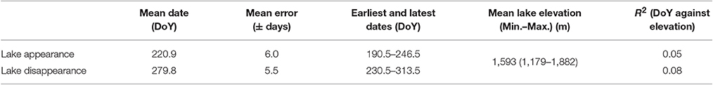
Table 4. Statistics from the subsurface lake appearance and disappearance detections from the Sentinel-1 data. DoY refers to day of year (in 2015).

The mean appearance date of the subsurface lakes is late in the ablation season (9 August), while the mean disappearance date is approaching the winter (7 October). As with surface lake freeze-through, there is no statistically significant correlation between the date of either subsurface lake appearance or disappearance with elevation (Table 4). The errors associated with the dates of subsurface lake appearance and disappearance increase at the highest elevations in the south of the study region (Supplementary Figures 5C,D) due to a restricted number of Sentinel-1 scenes over this area. This is also reflected in the mean error for the subsurface lake appearance and disappearance dates (±6.0 and ±5.5 days, respectively; Table 4), which is higher than the mean error of surface lake drainage dates (±4.0 days; Table 2) and freeze-through dates (±3.9 days; Table 3) from the Sentinel-1 dataset. The largest subsurface lake detected (15.9 km²) is more than double the size of the largest surface lake. Figure 10 shows the comparative sizes of surface and subsurface lakes for all of the identified lakes over the full study region.

FIGURE 10

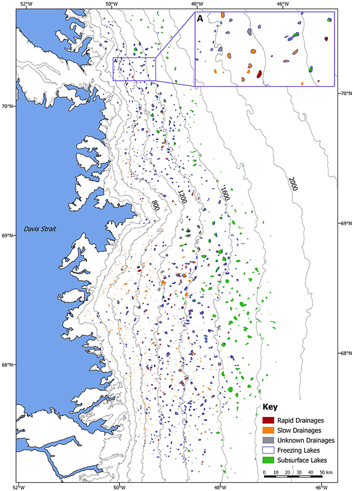
Figure 10. All types of supraglacial lakes (surface and subsurface) plotted over the full study region shown in Figure 1. Draining surface lakes are mapped using the combined Landsat–Sentinel-1 dataset; freezing surface lakes and subsurface lakes are mapped using the Sentinel-1 dataset only. Due to the overlap between the drainage and freeze-through datasets, grey, lakes with a blue border freeze-through only, whereas red and orange lakes with a blue border both drain and freeze-through during 2015. (A) Shows an enlarged subset of all lake types.

Discussion

Lake Detection

Sentinel-1's ability to image through clouds and in the dark, together with its higher temporal resolution than Landsat and higher spatial resolution than MODIS make it a valuable tool in the mapping of surface lakes on the GrIS. In our study, the mean lake size identified from Sentinel-1 (0.115 km²) was smaller than the minimum lake size used in most MODIS studies (0.125 km²). We were able to detect 2,297 lakes within the Sentinel-1 dataset over a study region of ~42,000 km². This compares to the detection of 1,120 lakes across the whole of west-southwest Greenland (an area approximately three times greater in size) by Selmes et al. (2011) using MODIS.

Sentinel-1 has a dual-polarization capability and it is important to understand how lakes appear in the two polarizations, and the implications of this for mapping lake areas. We identified three instances (the examples shown in Figure 8) where particular care is needed in detecting lakes from Sentinel-1 imagery. It is known that several factors affect radar backscatter, including seasonal timing of acquisition, look direction, incidence angle, surface and near-surface moisture, dielectric constant, and the structure/composition of the surface features (White et al., 2015). Furthermore, these properties can affect different radar polarizations in different ways. First, we interpret instances of widespread and consistently high and uniform backscatter across lakes in the HH polarization but not in the HV polarization (Figures 8A–C) as a product of wind-induced surface waves on the lake. In these circumstances, the HV polarization can better map open water because the backscatter is less dependent on surface roughness (Scheuchl et al., 2004) and is largely independent of incidence angle and wind direction (Vachon and Wolfe, 2011).

Second, we interpret instances of invisible lakes in the HH polarization but visible in the HV polarization (Figures 8D–F, red circles) in terms of a particular structure/composition of the ice-sheet surface. These instances typically occur in the upper ablation area, where wet snow and firn give a low dielectric contrast between the lakes and surrounding areas. Furthermore, topography is undulating in these areas, suggesting that the backscatter from the surface roughness features masks that associated with the presence of water (Töyrä and Pietroniro, 2005). Finally, this effect is more common in images with a low incidence angle, suggesting that these causes are exacerbated at shallow look angles. The HV backscatter response is largely unaffected due to its greater signal-to-noise ratio (Partington et al., 2010; Nagler et al., 2015, 2016). Third, we interpret instances of dispersed areas of very low backscatter, typical of that associated with lakes but where no lakes are visible (Figures 8D–F, green circles), in terms of subsurface water. These instances typically appear in the upper ablation area and lower accumulation area, where contemporaneous Landsat imagery suggests that there may be deep snow-filled surface depressions, and where the later imagery often depicts the presence of surface water.

Despite the instances where Sentinel-1 has difficulty detecting lakes, particularly in the HH polarization, our surface lake detection method performs well at determining total lake areas that are comparable to those derived by the Landsat NDWI classification (Figure 7). The overestimation of the total area derived by Sentinel-1 compared to Landsat (Table 1) is likely due to Sentinel-1 detecting shallower lake water in addition to the deeper water identified by the NDWI classification with its threshold value of 0.5. A lower NDWI threshold would have delineated more water and may have reduced this lake area difference.

The Sentinel-1 lake detection method could be improved in several ways. First, the application of the Landsat-derived composite lake mask with a fixed dilation value may have obscured the bimodal histogram distribution between water and ice backscatter, which led to the discarding of five of the Sentinel-1 images. This effect was greatest at the start and end of the melt season, where smaller lake areas were surrounded by a greater number of ice pixels within each Landsat-detected maximum lake area. Our small buffer of two pixels minimized this although, for future work, the use of a dynamic dilation proportional to lake size through the melt season would reduce the number of ice pixels and may perform better. Alternatively, it might be possible to determine a threshold value directly from the Sentinel-1 images that distinguishes water and slush, suppressing the need for the Landsat mask. Second, we were unable to independently validate the Sentinel-1 lake detection method against the Landsat NDWI due to the use of the Landsat lake detections as a mask in the Sentinel-1 procedure (Figure 2E). Including additional high-resolution imagery, such as Sentinel-2 or WorldView, or lake perimeters from field data, would allow an entirely independent validation of the Sentinel-1 lake detection method. This would subsequently provide greater confidence in the Sentinel-1-derived lake areas. Third, higher effective spatial resolution could be obtained for the Sentinel-1 imagery if a finer-resolution DEM were used in the pre-processing stages, potentially resulting in the Sentinel-1 imagery having superior spatial resolution to Landsat.

Lake Drainage

The very small number of rapid drainage events, and the large errors associated with the timing of the slow drainage dates for the Landsat analyses highlights the much lower temporal resolution of the Landsat images compared to the Sentinel-1 and combination datasets (Table 2). The very small error associated with the rapid drainage dates (±1.0 days; Table 2) is therefore an artifact of the small number of events that could be detected. Many of the slow drainages detected by the Landsat analysis may have been included erroneously, as snowfall events would have prevented the NDWI from detecting water; these may consequently have been marked as slow drainages, with this effect potentially also affecting the combination analysis due to its inclusion of Landsat data. By comparison, the Sentinel-1 dataset detected many more rapid drainage events, as well as identifying their drainage dates with higher certainty (Table 2). Sentinel-1 can image through fresh snow, providing a further advantage over Landsat in allowing accurate determination of slow lake drainage events at any point during the melt season. The number of rapid drainage events identified from the combined dataset was greater still, and the error associated with defining the drainage dates was consequently small. The low mean errors produced from the Sentinel-1 and combination analyses reflect their superior temporal resolution compared to the Landsat analysis, and therefore their greater suitability for assessing rapid changes to surface lakes.

The temporal resolution of the combined dataset (3.1 days as a seasonal average) is approaching that of MODIS's daily resolution and may even exceed MODIS's effective temporal resolution due to MODIS's inability to image through cloud. Our rapid lake drainage results are comparable to those from previous work based on MODIS. Of our total lake population, 22% were defined as draining rapidly (11% large and 11% small lakes). The 11% large rapid drainage events is similar to Selmes et al.'s (2011) 13% for the whole of southwest Greenland over 2005–2009, Fitzpatrick et al.'s (2014) 28% for Russell Glacier over eleven melt seasons, and Williamson et al.'s (2017) 21% for the Paakitsoq region and 15% for the Store Glacier region for the 2014 ablation season, all based on MODIS. However, we observed an additional 11% rapid drainage events for small lakes (<0.125 km²), which would have been missed in these MODIS-based studies.

The mean rapid drainage dates obtained from our combined Landsat–Sentinel-1 analysis further highlights the advantages of this dataset over MODIS data. We observe that the mean drainage date of small, rapidly draining lakes occurs earlier (27 July ±1.3 days) than for larger lakes (2 August ±1.6 days; Table 2). Morriss et al. (2013) used MODIS imagery to study rapid drainage events from 2002 to 2011 over West Greenland, generally finding that many rapid drainage events occurred in early to mid-July. However, between 2004 and 2008 they observed a number of events clustering in early to mid-August, and in 2007 they even observed a cluster in early September. Furthermore, Williamson et al. (2017) obtain mean drainage dates during 2014 of 12 July and 7 July for the Paakitsoq and Store Glacier regions, respectively, from MODIS data. However, they note that few drainages were observed beyond 18 July due to widespread cloud cover in these regions. Thus, our combined Landsat–Sentinel-1-derived mean drainage date for large lakes is likely more accurate than MODIS-derived dates, which are affected by cloud.

The combined dataset detected a greater number of slow lake drainage events (57%) at a lower mean elevation when compared to the rapid drainage events, similar to the results of Selmes et al. (2013). Slow lake drainages also occurred across a wider elevation range than rapid events (Figure 10). This might point to a glaciological control preventing rapid drainage events at low elevations. Lake area and volume is primarily controlled by the ice-surface topography, which varies with ice-sheet elevation (Chu, 2014). Towards the ice-sheet edge, the surface is steeper than the interior, and large depressions are rare (Sundal et al., 2009). Lakes forming in these locations are more likely to overflow and drain slowly, perhaps because the depressions are too small to reach the critical water volume necessary to initiate hydrofracture (Krawczynski et al., 2009) or because water inputs via nearby crevasses/moulins are incapable of causing the basal slip or uplift necessary to generate tensile fracture across the lake basins (Stevens et al., 2015).

The combined Landsat–Sentinel-1 dataset allowed small surface lake areas to be tracked at the high spatial resolution of both sensors. Thus, lake areas were tracked that were smaller (mean 0.089 km²) than those resolvable in MODIS (minimum size 0.125 km²). The mean elevation of small draining lakes is 159 m lower than for large lake drainages, for both rapid and slow draining lakes (Table 2). Therefore, previous work using MODIS may not have considered the full span of GrIS lake drainages due to its low spatial resolution, limiting the minimum trackable lake size to the size of the “large lakes” in this study. Models of the basal hydrology or basal drag of the GrIS require accurate calculations of the locations, timings and magnitudes of surface water inputs (Schoof, 2010; Hewitt, 2013; Werder et al., 2013; Banwell et al., 2016; Koziol et al., 2017). Our work holds promise in providing a methodology for deriving a dataset that can be used to either prescribe accurate surface water inputs to ice-sheet models, or for testing algorithms of surface melt, routing and lake drainage that can provide such inputs.

Lake Freeze-Through

Surface lake freeze-through dates could be manually identified from the Sentinel-1 imagery. This has been limited in previous studies that used optical sensors due to their inability to image late in the summer when cloud cover is high, solar illumination is low, and snowfall is common. Previous freeze-through studies have used proxies, such as the MODIS Land Surface Temperature product, to distinguish between freeze-through and slow lake drainage on the assumption that freeze-through occurs once the temperature drops below a defined threshold (Selmes et al., 2013). These approaches are therefore likely introduce errors. Accurate detection of freeze-through dates from the Landsat imagery in this study was impossible after the snowfall on day 228 (Figure 4). By contrast, Sentinel-1 can penetrate the shallow snow cover to return the backscatter signal of liquid water beneath, allowing more accurate freeze-through dates to be determined, even during periods of heavy cloud cover (Supplementary Figure 4).

The mean elevation of lake freeze-through was 1,270 m, similar to the ~1,500 m reported in 2005–2009 using MODIS across the whole of west-southwest Greenland (Selmes et al., 2013). Additionally, the mean elevation of freezing lakes is ~100 m higher than that for draining lakes (Tables 2, 3); in the MODIS study, this difference was ~200 m (Selmes et al., 2013). There was no statistically significant trend with elevation (Table 3; Supplementary Figure 4), suggesting that factors other than, or in addition to, the lapse rate control lake freeze-through.

The highest freezing lake elevation observed in this study was 1,712 m and, in general, lakes froze at higher elevations than those that drained (Figure 10). Sundal et al. (2009) found virtually no surface lakes above 1,600 m during the 2003 melt season, yet our study found a number of lakes above 1,600 m, some of which drained and the rest of which froze-through during 2015. The higher surface lake elevations observed in our study compared to Sundal et al. (2009) is in line with other work that indicates an increasing presence of water at higher elevations with increasing air temperatures (Bartholomew et al., 2010; Howat et al., 2013; Morriss et al., 2013; Fitzpatrick et al., 2014). If these higher elevation lakes increasingly drain rapidly rather than freeze-through, they could increase ice velocities in the short term if the water is accommodated in an enlarging subglacial cavity network (Zwally et al., 2002; Doyle et al., 2014), or decrease velocities in the long term if discharges are sufficient to cause channelization (Bartholomew et al., 2012; Sole et al., 2013). An improved understanding of the precise controls on hydrofracture would help to estimate whether surface lakes will be able to drain at these higher elevations in the future.

Subsurface Lakes

The only previous investigation of subsurface lakes used the IceBridge Snow Radar to assess subsurface lake depths, but it was unable to calculate their areal extents (Koenig et al., 2015). Sentinel-1 imagery has not only allowed subsurface lake areas to be measured, but has also allowed their seasonal lifespan to be calculated. Compared to the surface lakes that either drain or freeze, subsurface lakes appear quite late in the melt season, after the majority of drainage events have occurred (Tables 2–4; Supplementary Figure 5). Subsurface lakes freeze in the early winter, much later than the freeze-through of surface lakes, and are present at generally higher elevations than the surface lakes (Figure 10). The subsurface lakes extend up to nearly 1,900 m, with an elevation range of 1,179–1,882 m (Table 4); Koenig et al. (2015) also mapped the majority of their buried lakes between 1,000 and 2,000 m, and did not observe any above 2,000 m.

Although, the Sentinel-1-detected subsurface lakes show a similar distribution and density to those detected by IceBridge (Figure 9), the C-band SAR of Sentinel-1 is biased toward shallower subsurface features, while the L-band radar of IceBridge images deeper features. The similar distribution and density of these features for three years of IceBridge data and one year of Sentinel-1 data suggests that IceBridge only detected up to a third of the features due to its restricted flight line coverage, despite its greater penetration depth. Koenig et al. (2015) concluded that liquid water buried in lakes is present throughout the winter. Our work has allowed an analysis of lake behavior into the winter, and due to the late mean date of lake disappearance (7 October), we assume these lakes freeze-through. The discrepancy in the results may be due to the different penetration depths of the C-band and L-band radars, and/or the data extending to different dates in the autumn and early winter. The later freeze-through dates of subsurface lakes (7 October) compared to surface lakes (30 August) is likely due to the greater insulating effect of snow cover over the former compared to the latter. As also noted for the draining and freezing lakes, there is no statistically significant relationship between the date of subsurface lake appearance or disappearance with elevation, suggesting that factors other than or additional to the lapse rate control freeze-through. Thus, Sentinel-1 imagery allows the lifespan of the buried lakes to be determined, enhancing knowledge about the year-round distribution of liquid water within the surface layers of the GrIS.

Conclusions

In this study, Sentinel-1A SAR and Landsat-8 OLI imagery was used to investigate the behavior of surface and subsurface lakes in West Greenland. Where overlapping imagery was present, our semi-automated method of lake detection from Sentinel-1 imagery produced comparable results to a Landsat NDWI classification. Compared to the usable Landsat imagery, the Sentinel-1 dataset has a similar spatial resolution but a higher temporal resolution, and extends further into the summer and beyond into winter. This is due to the ability of the Sentinel-1 SAR to image through cloud and in darkness, unlike the optical Landsat sensor. Consequently, our Sentinel-1 lake detection method could identify smaller lakes than is possible with MODIS alone, and at a higher temporal resolution than is possible with Landsat imagery alone.

The combined Landsat–Sentinel-1 dataset has a higher spatial resolution but a near-comparable temporal resolution to MODIS imagery (three vs. one day, respectively) that has been used previously to investigate GrIS lake behavior (Selmes et al., 2011; Liang et al., 2012; Fitzpatrick et al., 2014; Williamson et al., 2017). The combined dataset could therefore detect and investigate the behavior of small lakes (<0.125 km²) that drained both rapidly and slowly, as well as large lakes that are visible in MODIS imagery. Our results show that smaller lakes drain slightly earlier in the melt season at lower elevations than large lakes. Thus, previous studies of lake drainage timing using MODIS would likely have been biased because of their inability to detect these smaller lakes, despite their importance for opening surface-to-bed connections that can receive meltwater for the remainder of the melt season.

The Sentinel-1 dataset was also used to detect the timing of surface lake freeze-through, which has previously been limited due to cloud and snow cover obscuring lakes in optical imagery. Lakes that froze over were more numerous and tended to be present at higher elevations than those that drained; however, no statistically significant trend was found between the date of freeze-through and elevation. Its ability to detect freezing lakes, and also subsurface lakes, at higher elevations than previously observed, and its ability to continue monitoring into the early winter makes Sentinel-1 SAR an ideal sensor for detecting supraglacial lake dynamics. The sensor allowed for the identification of the area and lifespan of subsurface lakes, which has not previously been observed. The mean freeze-through date of these lakes was 7 October, but the persistence of some until early November shows that liquid water is present longer than previously thought on the surface of the GrIS, with implications for the surface mass balance. Further work on these subsurface lakes would help to constrain these features and contribute to a better understanding of the surface hydrology of the GrIS. The temporal resolution of Sentinel is now even higher than used in this study, due to the launch of Sentinel-1B, further increasing its suitability for surface and subsurface lake detections on the GrIS.

Author Contributions

All authors contributed to this work. KM, IW, CB, and MT contributed to initial ideas and methodological developments. KM undertook the majority of the analysis and wrote the paper based on her M.Phil. thesis (University of Cambridge). AW wrote the FAST algorithm to detect lake drainage events, and adapted it for use with the Sentinel-1 and Landsat imagery. All authors contributed to the editing of the paper.

Conflict of Interest Statement

The authors declare that the research was conducted in the absence of any commercial or financial relationships that could be construed as a potential conflict of interest.

Acknowledgments

We thank Neil Arnold and Gareth Rees (Scott Polar Research Institute, University of Cambridge) and Yves-Louis Desnos (European Space Agency) for their useful advice on various aspects of this work. KM thanks Lucy Cavendish College (University of Cambridge) and the BB Roberts and William Vaughan Lewis Funds for financial assistance to attend the European Geosciences Union General Assembly 2016, where preliminary findings were presented and valuable feedback obtained. AW was funded by a UK Natural Environment Research Council Ph.D. studentship awarded through the Cambridge Earth System Science Doctoral Training Partnership (grant number: NE/L002507/1). We thank Andrew Sole, Matthias Braun and an anonymous reviewer for their thorough and helpful reviews that resulted in a considerably improved paper.

Supplementary Material

The Supplementary Material for this article can be found online at: https://www.frontiersin.org/article/10.3389/feart.2017.00058/full#supplementary-material

References

Arnold, N. S., Banwell, A. F., and Willis, I. C. (2014). High-resolution modelling of the seasonal evolution of surface water storage on the Greenland Ice Sheet. Cryosphere 8, 1149–1160. doi: 10.5194/tc-8-1149-2014

CrossRef Full Text | Google Scholar

Banwell, A. F., Caballero, M., Arnold, N. S., Glasser, N. F., Mac Cathles, L., and MacAyeal, D. R. (2014). Supraglacial lakes on the Larsen B ice shelf, Antarctica, and at Paakitsoq, West Greenland: a comparative study. Ann. Glaciol. 55, 1–8. doi: 10.3189/2014AoG66A049

CrossRef Full Text | Google Scholar

Banwell, A. F., Hewitt, I., Willis, I., and Arnold, N. (2016). Moulin density controls drainage development beneath the Greenland Ice Sheet. J. Geophys. Res. 121, 2248–2269. doi: 10.1002/2015JF003801

CrossRef Full Text | Google Scholar

Bartholomew, I., Nienow, P., Mair, D., Hubbard, A., King, M. A., and Sole, A. (2010). Seasonal evolution of subglacial drainage and acceleration in a Greenland outlet glacier. Nat. Geosci. 3, 408–411. doi: 10.1038/ngeo863

CrossRef Full Text | Google Scholar

Bartholomew, I., Nienow, P., Sole, A., Mair, D., Cowton, T., and King, M. A. (2012). Short-term variability in Greenland Ice Sheet motion forced by time-varying meltwater drainage: implications for the relationship between subglacial drainage system behavior and ice velocity. J. Geophys. Res. 117, 1–17. doi: 10.1029/2011jf002220

CrossRef Full Text | Google Scholar

Bindschadler, R., and Vornberger, P. (1992). Interpretation of SAR imagery of the Greenland Ice Sheet using coregistered TM imagery. Remote Sens. Environ. 42, 167–175. doi: 10.1016/0034-4257(92)90100-X

CrossRef Full Text | Google Scholar

Box, J. E., and Ski, K. (2007). Remote sounding of Greenland supraglacial melt lakes: implications for subglacial hydraulics. J. Glaciol. 53, 257–265. doi: 10.3189/172756507782202883

CrossRef Full Text | Google Scholar

Chu, V. W. (2014). Greenland ice sheet hydrology: a review. Progr. Phys. Geogr. 38, 19–54. doi: 10.1177/0309133313507075

CrossRef Full Text | Google Scholar

Csatho, B. M., Schenk, A. F., van der Veen, C. J., Babonis, G., Duncan, K., Rezvanbehbahani, S., et al. (2014). Laser altimetry reveals complex pattern of Greenland Ice Sheet dynamics. Proc. Natl. Acad. Sci. U.S.A. 111, 18478–18483. doi: 10.1073/pnas.1411680112

PubMed Abstract | CrossRef Full Text | Google Scholar

Copernicus (2016). Sentinels Scientific Data Hub. Available online at: https://scihub.copernicus.eu/ (Accessed February 1, 2016).

Das, S., Joughin, I., Behn, M., Howat, I., King, M., Lizarralde, D., et al. (2008). Fracture propagation to the base of the Greenland Ice Sheet during supraglacial lake drainage. Science 320, 778–782. doi: 10.1126/science.1153360

PubMed Abstract | CrossRef Full Text | Google Scholar

Dow, C. F., Kulessa, B., Rutt, I. C., Tsai, V. C., Pimentel, S., Doyle, S. H., et al. (2015). Modeling of subglacial hydrological development following rapid supraglacial lake drainage. J. Geophys. Res. 120, 1127–1147. doi: 10.1002/2014jf003333

PubMed Abstract | CrossRef Full Text | Google Scholar

Doyle, S., Hubbard, A., Fitzpatrick, A., van As, D., Mikkelsen, A., Pettersson, R., et al. (2014). Persistent flow acceleration within the interior of the Greenland ice sheet. Geophys. Res. Lett. 41, 899–905. doi: 10.1002/2013GL058933

CrossRef Full Text | Google Scholar

Doyle, S. H., Hubbard, A. L., Dow, C. F., Jones, G. A., Fitzpatrick, A., Gusmeroli, A., et al. (2013). Ice tectonic deformation during the rapid in situ drainage of a supraglacial lake on the Greenland Ice Sheet. Cryosphere 7, 129–140. doi: 10.5194/tc-7-129-2013

CrossRef Full Text | Google Scholar

Echelmeyer, K., Clarke, T. S., and Harrison, W. D. (1991). Surficial glaciology of Jakobshavn Isbrae, West Greenland: part I. Surface Morphology. J. Glaciol. 37, 368–382. doi: 10.1017/S0022143000005803

CrossRef Full Text | Google Scholar

Enderlin, E., Howat, I., Jeong, S., Noh, M. J., van Angelen, J., and van den Broeke, M. (2014). An improved mass budget for the Greenland Ice Sheet. Geophys. Res. Lett. 41, 866–872. doi: 10.1002/2013GL059010

CrossRef Full Text | Google Scholar

Fitzpatrick, A. A. W., Hubbard, A. L., Box, J. E., Quincey, D. J., Van As, D., Mikkelsen, A. P. B., et al. (2014). A decade (2002-2012) of supraglacial lake volume estimates across Russell Glacier, West Greenland. Cryosphere 8, 107–121. doi: 10.5194/tc-8-107-2014

CrossRef Full Text | Google Scholar

Georgiou, S., Shepherd, A., McMillan, M., and Nienow, P. (2009). Seasonal evolution of supraglacial lake volume from ASTER imagery. Ann. Glaciol. 50, 95–100. doi: 10.3189/172756409789624328

CrossRef Full Text | Google Scholar

Hewitt, I. (2013). Seasonal changes in ice sheet motion due to melt water lubrication. Earth Planet. Sci. Lett. 371–372, 16–25. doi: 10.1016/j.epsl.2013.04.022

CrossRef Full Text

Hirose, T., Kapfer, M., Bennett, J., Cott, P., Manson, G., and Solomon, S. (2008). Bottomfast ice mapping and the measurement of ice thickness on tundra lakes using C-band synthetic aperture radar remote sensing. J. Am. Water Resour. Assoc. 44, 285–292. doi: 10.1111/j.1752-1688.2007.00161.x

CrossRef Full Text | Google Scholar

Howat, I. M., de la Peña, S., van Angelen, J. H., Lenaerts, J. T. M., and van den Broeke, M. R. (2013). Brief communication “Expansion of meltwater lakes on the Greenland Ice Sheet.” Cryosphere 7, 201–204. doi: 10.5194/tcd-6-4447-2012

CrossRef Full Text | Google Scholar

Howat, I. M., Negrete, A., and Smith, B. E. (2014). The Greenland Ice Mapping Project (GIMP) land classification and surface elevation data sets. Cryosphere 8, 1509–1518. doi: 10.5194/tc-8-1509-2014

CrossRef Full Text | Google Scholar

Huggel, C., Kääb, A., Haeberli, W., Teysseire, P., and Paul, F. (2002). Remote sensing based assessment of hazards from glacier lake outbursts: a case study in the Swiss Alps. Can. Geotech. J. 39, 316–330. doi: 10.1139/t01-099

CrossRef Full Text | Google Scholar

Johansson, A. M., and Brown, I. A. (2012). Observations of supra-glacial lakes in west Greenland using winter wide swath Synthetic Aperture Radar. Remote Sens. Lett. 3, 531–539. doi: 10.1080/01431161.2011.637527

CrossRef Full Text | Google Scholar

Johansson, A. M., Jansson, P., and Brown, I. A. (2013). Spatial and temporal variations in lakes on the Greenland Ice Sheet. J. Hydrol. 476, 314–320. doi: 10.1016/j.jhydrol.2012.10.045

CrossRef Full Text | Google Scholar

Joughin, I., Das, S., King, M., Smith, B., Howat, I., and Moon, T. (2008). Seasonal speedup along the western flank of the Greenland Ice Sheet. Science 320, 781–783. doi: 10.1126/science.1153288

PubMed Abstract | CrossRef Full Text | Google Scholar

Joughin, I., Das, S. B., Flowers, G. E., Behn, M. D., Alley, R. B., King, M. A., et al. (2013). Influence of ice-sheet geometry and supraglacial lakes on seasonal ice-flow variability. Cryosphere 7, 1185–1192. doi: 10.5194/tc-7-1185-2013

CrossRef Full Text | Google Scholar

Koenig, L. S., Lampkin, D. J., Montgomery, L. N., Hamilton, S. L., Turrin, J. B., Joseph, C. A., et al. (2015). Wintertime storage of water in buried supraglacial lakes across the Greenland Ice Sheet. Cryosphere 9, 1333–1342. doi: 10.5194/tc-9-1333-2015

CrossRef Full Text | Google Scholar

König, M., Winther, J.-G., and Isaksson, E. (2001). Measuring snow and glacier ice properties from satellite. Rev. Geophys. 39, 1–27. doi: 10.1029/1999RG000076

CrossRef Full Text | Google Scholar

Koziol, C., Arnold, N., Pope, A., and Colgan, W. (2017). Quantifying supraglacial meltwater pathways in the Paakitsoq region, West Greenland. J. Glaciol. 63, 464–476. doi: 10.1017/jog.2017.5

CrossRef Full Text | Google Scholar

Krawczynski, M. J., Behn, M. D., Das, S. B., and Joughin, I. (2009). Constraints on the lake volume required for hydro-fracture through ice sheets. Geophys. Res. Lett. 36, 1–5. doi: 10.1029/2008GL036765

CrossRef Full Text | Google Scholar

Leeson, A., Shepherd, A., Briggs, K., Howat, I., Fettweis, X., Morlighem, M., et al. (2015). Supraglacial lakes on the Greenland ice sheet advance inland under warming climate. Nat. Clim. Chang. 5, 51–55. doi: 10.1038/nclimate2463

CrossRef Full Text | Google Scholar

Lewis, S., and Smith, L. (2009). Hydrological drainage of the Greenland Ice Sheet. Hydrol. Process. 23, 2004–2011. doi: 10.1002/hyp.7343

CrossRef Full Text | Google Scholar

Liang, Y.-L., Colgan, W., Lv, Q., Steffen, K., Abdalati, W., Stroeve, J., et al. (2012). A decadal investigation of supraglacial lakes in West Greenland using a fully automatic detection and tracking algorithm. Remote Sens. Environ. 123, 127–138. doi: 10.1016/j.rse.2012.03.020

CrossRef Full Text | Google Scholar

Luckman, A., Elvidge, A., Jansen, D., Kulessa, B., Kuipers Munneke, P., King, J., et al. (2014). Surface melt and ponding on Larsen C Ice Shelf and the impact of föhn winds. Antarct. Sci. 26, 625–635. doi: 10.1017/S0954102014000339

CrossRef Full Text | Google Scholar

Lüthje, M., Pedersen, L. T., Reeh, N., and Greuell, W. (2006). Modelling the evolution of supraglacial lakes on the west Greenland ice-sheet margin. J. Glaciol. 52, 608–618. doi: 10.3189/172756506781828386

CrossRef Full Text | Google Scholar

Mayaud, J. R., Banwell, A. F., Arnold, N. S., and Willis, I. C. (2014). Modeling the response of subglacial drainage at Paakitsoq, west Greenland, to 21st century climate change. J. Geophys. Res. 119, 2619–2634. doi: 10.1002/2014JF003271

CrossRef Full Text | Google Scholar

McMillan, M., Nienow, P., Shepherd, A., Benham, T., and Sole, A. (2007). Seasonal evolution of supra-glacial lakes on the Greenland Ice Sheet. Earth Planet. Sci. Lett. 262, 484–492. doi: 10.1016/j.epsl.2007.08.002

CrossRef Full Text | Google Scholar

Morriss, B. F., Hawley, R. L., Chipman, J. W., Andrews, L. C., Catania, G. A., Hoffman, M. J., et al. (2013). A ten-year record of supraglacial lake evolution and rapid drainage in West Greenland using an automated processing algorithm for multispectral imagery. Cryosphere 7, 1869–1877. doi: 10.5194/tc-7-1869-2013

CrossRef Full Text | Google Scholar

Moussavi, M. S., Abdalati, W., Pope, A., Scambos, T., Tedesco, M., MacFerrin, M., et al. (2016). Derivation and validation of supraglacial lake volumes on the Greenland Ice Sheet from high-resolution satellite imagery. Remote Sens. Environ. 183, 294–303. doi: 10.1016/j.rse.2016.05.024

CrossRef Full Text | Google Scholar

Nagler, T., Rott, H., Hetzenecker, M., Wuite, J., and Potin, P. (2015). The sentinel-1 mission: new opportunities for ice sheet observations. Remote Sens. 7, 9371–9389. doi: 10.3390/rs70709371

CrossRef Full Text | Google Scholar

Nagler, T., Rott, H., Ripper, E., Bippus, G., and Hetzenecker, M. (2016). Advancements for snowmelt monitoring by means of sentinel-1 SAR. Remote Sens. 8:348. doi: 10.3390/rs8040348

CrossRef Full Text | Google Scholar

Partington, K. C., Flach, J. D., Barber, D., Isleifson, D., Meadows, P. J., and Verlaan, P. (2010). Dual-polarization C-band radar observations of sea ice in the Amundsen Gulf. IEEE Trans. Geosci. Remote Sens. 48, 2685–2691. doi: 10.1109/TGRS.2009.2039577

CrossRef Full Text | Google Scholar

Pope, A., Scambos, T. A., Moussavi, M., Tedesco, M., Willis, M., Shean, D., et al. (2016). Estimating supraglacial lake depth in West Greenland using Landsat 8 and comparison with other multispectral methods. Cryosphere 10, 15–27. doi: 10.5194/tc-10-15-2016

CrossRef Full Text | Google Scholar

Rennermalm, A. K., Smith, L. C., Chu, V. W., Box, J. E., Forster, R. R., Van Den Broeke, M. R., et al. (2013). Evidence of meltwater retention within the Greenland ice sheet. Cryosphere 7, 1433–1445. doi: 10.5194/tc-7-1433-2013

CrossRef Full Text | Google Scholar

Rignot, E., Velicogna, I., van den Broeke, M. R., Monaghan, A., and Lenaerts, J. T. M. (2011). Acceleration of the contribution of the Greenland and Antarctic ice sheets to sea level rise. Geophys. Res. Lett. 38, 1–5. doi: 10.1029/2011gl046583

CrossRef Full Text | Google Scholar

Scheuchl, B., Flett, D., Caves, R., and Cumming, I. (2004). Potential of RADARSAT-2 data for operational sea ice monitoring. Can. J. Remote Sens. 30, 448–461. doi: 10.5589/m04-011

CrossRef Full Text | Google Scholar

Schoof, C. (2010). Ice-sheet acceleration driven by melt supply variability. Nature 468, 803–806. doi: 10.1038/nature09618

PubMed Abstract | CrossRef Full Text | Google Scholar

Selmes, N., Murray, T., and James, T. D. (2011). Fast draining lakes on the Greenland Ice Sheet. Geophys. Res. Lett. 38, 1–5. doi: 10.1029/2011GL047872

CrossRef Full Text | Google Scholar

Selmes, N., Murray, T., and James, T. D. (2013). Characterizing supraglacial lake drainage and freezing on the Greenland Ice Sheet. Cryosph. Discuss. 7, 475–505. doi: 10.5194/tcd-7-475-2013

CrossRef Full Text | Google Scholar

Sole, A., Nienow, P., Bartholomew, I., Mair, D., Cowton, T., Tedstone, A., et al. (2013). Winter motion mediates dynamic response of the Greenland Ice Sheet to warmer summers. Geophys. Res. Lett. 40, 3940–3944. doi: 10.1002/grl.50764

CrossRef Full Text | Google Scholar

Stevens, L. A., Behn, M. D., McGuire, J. J., Das, S. B., Joughin, I., Herring, T., et al. (2015). Greenland supraglacial lake drainages triggered by hydrologically induced basal slip. Nature 522, 73–76. doi: 10.1038/nature14480

PubMed Abstract | CrossRef Full Text | Google Scholar

Sundal, A. V., Shepherd, A., Nienow, P., Hanna, E., Palmer, S., and Huybrechts, P. (2009). Evolution of supra-glacial lakes across the Greenland Ice Sheet. Remote Sens. Environ. 113, 2164–2171. doi: 10.1016/j.rse.2009.05.018

CrossRef Full Text | Google Scholar

Tedesco, M., Lüthje, M., Steffen, K., Steiner, N., Fettweis, X., Willis, I., et al. (2012). Measurement and modeling of ablation of the bottom of supraglacial lakes in western Greenland. Geophys. Res. Lett. 39, 1–5. doi: 10.1029/2011GL049882

CrossRef Full Text | Google Scholar

Tedesco, M., and Steiner, N. (2011). In-situ multispectral and bathymetric measurements over a supraglacial lake in western Greenland using a remotely controlled watercraft. Cryosphere 5, 445–452. doi: 10.5194/tc-5-445-2011

CrossRef Full Text | Google Scholar

Tedesco, M., Willis, I. C., Hoffman, M. J., Banwell, A. F., Alexander, P., and Arnold, N. S. (2013). Ice dynamic response to two modes of surface lake drainage on the Greenland ice sheet. Environ. Res. Lett. 8:34007. doi: 10.1088/1748-9326/8/3/034007

CrossRef Full Text | Google Scholar

Tedstone, A. J., Nienow, P. W., Sole, A. J., Mair, D. W. F., Cowton, T. R., Bartholomew, I. D., et al. (2013). Greenland ice sheet motion insensitive to exceptional meltwater forcing. Proc. Natl. Acad. Sci. U.S.A. 110, 19719–19724. doi: 10.1073/pnas.1315843110

PubMed Abstract | CrossRef Full Text | Google Scholar

Töyrä, J., and Pietroniro, A. (2005). Towards operational monitoring of a northern wetland using geomatics-based techniques. Remote Sens. Environ. 97, 174–191. doi: 10.1016/j.rse.2005.03.012

CrossRef Full Text | Google Scholar

Vachon, P. W., and Wolfe, J. (2011). C-band cross-polarization wind speed retrieval. IEEE Trans. Geosci. Remote Sens. 8, 456–459. doi: 10.1109/LGRS.2010.2085417

CrossRef Full Text | Google Scholar

Vaughan, D. G., Comiso, J. C., Allison, I., Carrasco, J., Kaser, G., Kwok, R., et al. (2013). “Observations: cryosphere,” in Climate Change 2013: The Physical Science Basis. Contribution of Working Group I to the Fifth Assessment Report of the Intergovernmental Panel on Climate Change, eds T. F. Stocker, G.-K. D. Qin, M. Plattner, S. Tignor, K. Allen, J. Boschung, et al. (Cambridge, UK; New York, NY: Cambridge University Press), 317–382.

Google Scholar

Werder, M., Hewitt, I., Schoof, C., and Flowers, G. (2013). Modeling channelized and distributed subglacial drainage in two dimensions. J. Geophys. Res. Earth Surf. 118, 2140–2158. doi: 10.1002/jgrf.20146

CrossRef Full Text | Google Scholar

White, L., Brisco, B., Dabboor, M., Schmitt, A., and Pratt, A. (2015). A collection of SAR methodologies for monitoring wetlands. Remote Sens. 7, 7615–7645. doi: 10.3390/rs70607615

CrossRef Full Text | Google Scholar

Williamson, A. G., Arnold, N. S., Banwell, A. F., and Willis, I. C. (2017). A Fully Automated Supraglacial lake area and volume Tracking (“FAST”) algorithm: development and application using MODIS imagery of West Greenland. Remote Sens. Environ. 196, 113–133. doi: 10.1016/j.rse.2017.04.032

CrossRef Full Text | Google Scholar

Xu, H. (2006). Modification of normalised difference water index (NDWI) to enhance open water features in remotely sensed imagery. Int. J. Remote Sens. 27, 3025–3033. doi: 10.1080/01431160600589179

CrossRef Full Text | Google Scholar

Yang, K., and Smith, L. C. (2013). Supraglacial streams on the Greenland Ice Sheet delineated from combined spectral-shape information in high-resolution satellite imagery. IEEE Geosci. Remote Sens. Lett. 10, 801–805. doi: 10.1109/LGRS.2012.2224316

CrossRef Full Text | Google Scholar

Zwally, H. J., Abdalati, W., Herring, T., Larson, K., Saba, J., and Steffen, K. (2002). Surface melt-induced acceleration of Greenland ice-sheet flow. Science 297, 218–223. doi: 10.1126/science.1072708

PubMed Abstract | CrossRef Full Text | Google Scholar