Sclerochronological Study of a Glycymeris vangentsumi Population From the Madeira Islands

Introduction

It has been noted that sclerochronological analyses of mollusk shells are capable of providing high resolution archives of their marine environment (Schöne and Gillikin, 2013). Environmentally sensitive bivalve shells produce their shell carbonate on a periodic basis as seasonally occurring unfavorable environmental conditions leave recognizable marks in the shell structure. The cessation of growth results in growth lines. Sclerochronology, the analysis of skeletal growth patterns, can reveal changes in the growth rate of the shells and give us information about the changes in their ambient environment on a sub-seasonal scale (Richardson, 2001; Schöne et al., 2003).

If synchronous patterns can be observed in shell growth, bivalves with overlapping life-spans can be organized into shell-increment chronologies covering centuries or even millennia (Butler et al., 2013; Reynolds et al., 2013; Holland et al., 2014). These chronologies can be used for environmental reconstructions, if increment proxies can be successfully calibrated against instrumental temperature records (e.g., Reynolds et al., 2013). Due to the significant length of shell increment records, the impact of large-scale climate variability over centennial scales can be investigated by sclerochronological methods (Mette et al., 2016).

Glycymeris vangentsumi was only recently distinguished as a separate species based on morphometric features (Goud and Gulden, 2009). This species, endemic to the Macaronesian Shelf, was identified as Glycymeris glycymeris by earlier studies as it has similar features to its broadly researched co-genetic species. Due to the recentness of its discovery, information on the life-cycle of G. vangentsumi is sparse. Several Glycymeris species, however, are known to develop growth lines annually, such as G. glycymeris (Royer et al., 2013), G. bimaculata (Bušelić et al., 2015), and G. nummaria (Peharda et al., 2012) it is a logical expectation therefore that G. vangentsumi develops them as well. The formation of annual growth lines of G. glycymeris has been shown to be associated with decreasing temperatures in winter in the extratropical North Atlantic region (Brocas et al., 2013; Reynolds et al., 2013; Royer et al., 2013). Meanwhile annual growth lines have been observed to appear in early-spring in the Adriatic in G. bimaculata (Bušelić et al., 2015). Similarly, G. nummaria is known to form annual growth lines in February (Peharda et al., 2012).

The driving environmental factors for shell growth in the case of Glycymeris species were only studied so far in the extratropical North Atlantic and the Adriatic regions. Royer et al. (2013) established the minimum thermal threshold for G. glycymeris shell growth at 12.9°C temperature under which shell growth extremely slows down or stops. They also found a positive correlation between annual shell growth and sea surface temperature (SST), similarly to other sclerochronological studies conducted on Glycymeris species (Brocas et al., 2013; Reynolds et al., 2013; Bušelić et al., 2015). According to the aforementioned studies, low SST seems to be the key limiting factor for shell growth for Glycymeris species. However, a link between higher SST and increased shell growth rate, however, is not always evident. A G. glycymeris population studied from the Bay of Brest displayed no significant correlation between growth rates and SST. Rather, a link between enhanced shell growth and riverine nutrient input was put forward (Featherstone et al., 2017). Similarly, increased annual shell growth of G. pilosa was reported to correlate positively with precipitation (and the resulting enhancement in primary production) and negatively with summer SST from the Adriatic (Peharda et al., 2016).

The diversity in the nature of relations observed between shell growth and water temperature by different studies suggests that it may also depend on the shell's habitat. If primary production does not exclusively depend on SST but also on nutrient input, positive correlation between SST and shell growth will be less evident.

It seems reasonable to suggest that seasonal minima (relatively lower SSTs) could hardly be a limiting factor for Glycymeris spp. growth in a warm sub-tropical habitat. However, as the use of Glycymeris spp. in palaeoenvironmental modeling has already begun on fossil shells (Walliser et al., 2015), it is essential to examine the dominant environmental variables regulating annual growth under different climatic conditions for this genus. A pair of pertinent questions concerning the use of shells from poorly defined palaeodepths in future palaeoenvironmental reconstructions can be raised: Can Glycymeris shells living in habitats below the thermocline or a depth of ~100 m be affected by seasonal fluctuation of SST? And, if so, how?

In contrast to the extratropical North Atlantic, where multicentennial sclerochronological records support the reconstruction of certain parameters of the marine environment (Butler et al., 2013), the southern part of the North Atlantic still lacks shell-based composite chronologies, which might provide potential SST archives and valuable information on the main environmental variables of the region, such as the dynamics of the Canary Current System.

Faced with these challenges, the aims of this study were to analyse the annual growth patterns of Glycymeris vangentsumi shells, to obtain information about the longevity of this species, and to determine the most influential environmental variables affecting shell growth. Additionally, a specific aim was to compare the growth trends of shells collected at different depths but from the same location, in order to understand the effects of depth gradient on their juvenile growth rates.

Materials and Methods

Environmental Setting

The Madeira Islands (Madeira, Porto Santo, and the Desertas Islands) are part of a number of volcanic islands scattered along the Macaronesian Shelf (Figure 1A). The climate of the region is influenced by the North Atlantic subtropical gyre (Sverdrup, 1953) with the zonal Azores Current and its southward flowing branches. The axis of the Azores Current fluctuates seasonally and annually between 32 and 35°N in the Canary Basin (Figure 1B) as defined by its northern boundary, the Azores frontal region, the main element of mesoscale circulation in the region. The front meanders across the path of the Trade Winds (Lázaro et al., 2013), its position controlled by anticyclonic and cyclonic eddies. As the Trade Winds increase evaporation, the uppermost 200 m of the ocean is significantly warmer and more saline south of the Azores Front than north of the front (Fründt and Waniek, 2012). The meridional shifts of the Azores Front greatly affect primary production in the upper water column in the region, as the position of the front affects the depth and intensity of late-winter ocean-mixing in the region (Fründt and Waniek, 2012).

FIGURE 1

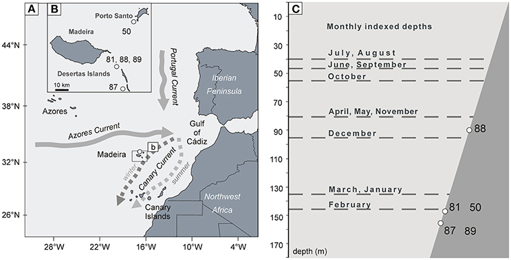
Figure 1. (A) Sketch map of the major ocean currents in the subtropical east Atlantic redrawn from Figure 1 in Mason et al. (2011). (B) The inset sketch map is focused on the Madeira Islands. The numbers indicate the shell collection sites around the islands. (C) Visualization of the relative vertical distribution of the sampling sites compared to the seasonally varying depth of the mixed layer (gray dashed lines); the data were taken from the Subduction Experiment moorings (Mason et al., 2011).

The Canary Current is a weaker, wind-driven eastern boundary current, which is considered to be a continuation of the Azores Current after its deflection toward the Equator by the African continent. It tends to flow far offshore in the vicinity of Madeira in winter, transporting cold water from the north, while in summer it occupies a more central position between Madeira and the African coast (Figure 1B) (Mason et al., 2011). When currents from NE direction become stronger, they deliver cooler water to the region, contributing to the phenomenon of late-winter mixing (Henson et al., 2009).

The collection sites were situated on the western slope of the Desertas Islands, at depths at depths comprised between 90 and 160 m (Figure 1C). In relation to other research conducted on Glycymeris spp. so far, this collection depth is uniquely low, and the resulting hydrographic differences between the shells' habitat and the sea surface should therefore also be taken into account. The late winter/early spring cooling of the SST and wind-mixing in the Canary Basin result in the late-winter mixing phenomenon (Figure 1C). Late-winter mixing means that during most of the year, these sub-tropical waters are stratified, as the depth of the mixed layer is situated at only around 50 m. In February and March, however, the mixing front penetrates to a depth of 130–150 m (Mason et al., 2011). While seasonal temperature variation is remarkable at the surface (Martins et al., 2007), it is not significant at the depth of the collection sites of this study, at which water temperature never exceeds 20°C (Mason et al., 2011).

The chlorophyll (Chl-a) content of the surface seawater in the region stands in an inverse relationship to the SST, following a pronounced seasonal pattern, with its maximum in February or March followed by a long period of low concentrations in the surface water between May and October. The maxima of surface Chl-a concentrations show a strong inter-annual variability, closely connected to the average SST of the corresponding months (Martins et al., 2007). Satellite-based estimates of chlorophyll concentration are available only for the uppermost layer of the water column while the depth of maximum chlorophyll concentration varies seasonally in the region through the upper 200 m of the water column (Teira et al., 2005). Environmental conditions at these depths are not monitored as regularly as at the surface, though in the last decade more data have been collected from cruises and at ocean moorings (Weller et al., 2004; Teira et al., 2005; Waniek et al., 2005). This has enabled the build-up of models of seasonal oceanographic processes (Mason et al., 2011; Fründt et al., 2015).

Phytoplankton blooms around Madeira are mainly influenced by late-winter mixing, since it enhances nutrient concentration in the euphotic zone. When the surface becomes nutrient-depleted in late-spring, phytoplankton descend to the lower part of the euphotic zone (90–130 m), where nutrients are still available, creating the deep chlorophyll maximum (DCM) (Teira et al., 2005), which usually persists through late summer and early autumn (Fründt et al., 2015), presumably still providing food for the mollusks living at that depth.

Shell Collection and Preparation

The CIIMAR-Madeira research cruise collected 58 single shells and two live Glycymeris specimens in March, 2014 at six sites using Shipek and Van Veen grabs off the coast of Madeira, near the Desertas Island at depths of 90–160 m (Figures 1B,C, see Data Sheet 1 for further details).

All the collected shells are symmetric and rounded; an angular posterior and well-rounded anterior can be still observed on the well preserved specimens. Shell length never exceeds 50 mm, which is unusually low for G. glycymeris, but falls within the range of the shell length of the G. vangentsumi (Goud and Gulden, 2009), just as in the case of their concavity (0.64 based on the average of 15 measurements).

All dead-collected specimens were unarticulated, showing different degrees of preservation. There was a remarkable difference in the degree of shell preservation between the different collection sites (Table 1). While even the larger shells with no pigmentation were relatively well preserved at Site 81, most shells collected from Site 87 were porous, discolored and cemented with sand and bio-clasts. Surprisingly, these sites were situated at the same depth (Figure 1C). The most porous shells from Site 87 were excluded from further investigations due to their increment records being heavily damaged. The relative difference of the state of preservation was used later as an ancillary information in the cross-correlation process.

TABLE 1

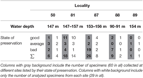
Table 1. Summary table of the distribution of the collected specimens among the collection sites and preservation categories.

Shells were glued to epoxy cubes, coated with quick-drying metal epoxy resin along the axis of maximum growth and cut axially to their ventral plains. Along this axis, a 3-mm section was cut from each specimen using a low-speed precision saw (Buehler Isomet 1000) equipped with a 0.4 mm diamond-coated wafering blade. Next, shell sections were mounted on glass slides with metal epoxy resin, grounded (400, 800, and 1,200 grit SiC powder) and polished (1 μm Al₂O₃ powder) and subsequently immersed for ca. 30 min under constant stirring in Mutvei's solution. This method includes etching (1% acetic-acid) and staining (alcian blue) simultaneously as growth lines are generally more resistant to etching and have higher organic material content (Schöne et al., 2005). Twenty seven shells were treated following this procedure, two other shell sections were prepared later using the acetate peel method: the polished surfaces were etched in 0.1 M HCl for 3 min, soaked in a water bath and left to air dry for a day. Acetate peels were made following the method described in Richardson (2001).

Cross-sections (n = 29) were photographed with a Canon EOS 550D digital camera attached to a Wild Heerbrugg M8 stereomicroscope equipped with sectoral dark field illumination (Schott VisiLED MC 1000).

Cross-Dating and Chronology Construction

Growth increments were measured along the hinge plate using digital photos and CooRecorder software (Larsson, 2014) (Figure 2). Most shells were collected from the 140-160 m depth range, however, collection site 88 was situated at 90–91 m depth (Figure 1, Table 1). By cross-dating shells only from the 140–160 depth range, the increment chronology was assumedly built from an ecologically more homogeneous sample set.

FIGURE 2

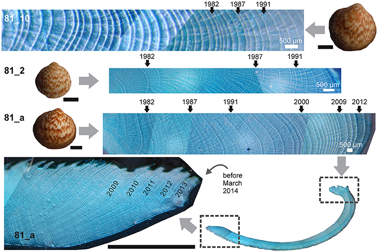
Figure 2. Annual increments in the hinge portions of three Mutvei-stained samples (where 81_a is the specimen collected alive) augmented with a close-up micrograph of the stained section of the ventral margin and a panorama picture of the height-parallel section of the same specimen. Index years are indicated on their corresponding annual increments. Scale bars are 1 cm for the accompanying photographs of G. vangentsumi specimens.

For the cross-dating process, the subfossil shells were sorted based on their different states of preservation to assign a relative sequence before cross-correlation (Table 1). Characteristic features were found to be as follows: (i) some of the shells still had their periostracum on the margin of the shell or pigmentation on their surface, (ii) other shells were completely colorless, showed signs of encrusting and boring biota, (iii) a large number of shells, especially from sample location 87, were cemented to the surrounding sediment or their structure became porous and friable.

Log-transformed individual increment records of the subfossil samples were visually cross-dated with those samples collected alive and having a fixed calendar date. The shells collected alive grew characteristically narrow increments labeled as 1982, and 1987 and broad increments labeled 1991, 2000, 2009, 2012 (Figure 2). These were used as primary markers in the first step of the increment synchronization. COFECHA software (Grissino-Mayer, 2001) was used to check the results of the visual cross-dating using 31-year windows with 25-year overlaps.

An adaptive power transformation was first applied to each time series to reduce the extreme heteroscedasticity of the raw data (Cook and Peters, 1997). Raw increment series were standardized to remove age related trends and growth disturbances resulting from population dynamics (Cook et al., 1990). In order to partially eliminate potential biases of a particular standardization technique, raw increment data have been processed by two alternative standardization methods:

(i) A negative exponential growth function, because this method is quite popular in sclerochronological studies and it was found to be least prone to filter out long-term variability in the growth of the shell (e.g., Marali and Schöne, 2015).

(ii) Hugershoff curve is an alternative approach when a polynomial-exponential combined function is fitted to the measured data and fitting parameters iteratively tuned (Warren, 1980). This function is capable to reproduce the accelerated growth at the juvenile growth (see Longevity and Ontogenetic Trends of the G. vangentsumi Population Near the Madeira Islands.) providing a challenge to the monotonic curves such as the linear- or the negative exponential functions.

Individual indices were derived as differences between the raw measurements and their fitted functions. Autoregressive modeling (Box and Jenkins, 1976) was applied to remove the lag 1 autocorrelation from each individual index. A pooled-autocorrelation model was determined for the cross-dated population and combined with mean chronology to add the lost persistence considered to be related to environmental signal (Cook, 1985). The mean chronology was calculated as a bi-weight robust mean (Mosteller and Tukey, 1977). Composite chronologies have been computed for both negative exponential and Hugershoff detrended chronologies and have been marked as NE and H, respectively. The robustness of the composite chronology was then assessed using interseries correlation (Rbar) and Expressed Population Signal (EPS) statistics calculated in 20-increment running windows. EPS estimates how well a finite number of analyzed samples represents the theoretical population average (Wigley et al., 1984). Note here, EPS is a valuable means for assessing the representation of the population signal, but it will not reveal whether this signal is closely related to any environmental parameter or any other source of common growth variation (Buras, 2017). Variance adjustment was applied to the derived chronologies to minimize variance bias due to changing sample replication and the effect of fluctuating interseries correlation (Osborn et al., 1997).

Detrending and index calculation procedures were carried out using ARSTAN software (Cook and Krusic, 2007), which constructed three composite chronologies (standardized, residual, and arstan) differing only in degrees reintegrated autoregressive modeling. Through this study, Arstan chronology was used for environmental analysis, which is produced by reincorporating the pooled autoregression (persistence) into the residual chronology. Both NE and H composite chronologies were compared to environmental variables potentially influencing the interannual variation of shell growth.

Environmental Variables and Applied Statistical Tools

Monthly SST data were extracted from the HadISST gridded product (Rayner et al., 2003) for the time interval 1950–2012 from the 17.0W-16.0W, 32.0N-33.0N grid cell covering Madeira. Weekly satellite-derived chlorophyll-a data were also obtained from the satellite data record of OSCAR (NASA, Physical Oceanography Program http://www.oceanmotion.org/html/resources/ssedv.htm) from 1998 to 2012 for the region of interest (16.0W-14.0W, 30.0N-32.0N). This data collection compiles data from the Moderate-resolution Imaging Spectroradiometer (MODIS) Aqua and the Sea-viewing Wide Field-of-view Sensor (SeaWiFS) estimating surface ocean productivity made available by the NASA Goddard Space Flight Center, Ocean Biology Processing Group (NASA, 2014). Annual mean total surface irradiation (TSI) data was obtained from the compilation based on Krivova et al. (2010) (http://www2.mps.mpg.de/projects/sun-climate/data.html).

The relationship between shell increment widths and monthly SST, TSI, satellite-derived Chl-a concentrations and the increment chronologies was evaluated by computing Pearson's correlation coefficients. Between annual shell growth indices and SST (HadISST), the coefficients were calculated from November of the previous year to December of the current year of increment formation, while in the case of the monthly satellite-derived Chl-a concentrations, from January to December. The spatial distribution of the strength of correlation between standardized shell increment records and SST was tracked using the KNMI Climate Explorer (Trouet and Van Oldenborgh, 2013) and the HadISST fields. The obtained correlation coefficients were compared to significance levels (p = 0.05) estimated using a two-tailed t-test for the corresponding degrees of freedom in order to assess the statistical significance.

Results

Longevity and Ontogenetic Trends of the G. vangentsumi Population Near the Madeira Islands

Age-aligned individual increment records displayed a characteristic pattern of reduction of growth with age (Figure 3A). Following a juvenile period of relatively rapid shell growth, average increment width declines in all groups. In groups 50, 81, and 87 (with samples collected from depths between 147 and 157 m) maximum increment width was 200–300 μm (Figure 3A). However, in the two shells from group 88, collected at 90 m, the broadest increment was 450–800 μm wide (Figure 3A). Increment widths in all groups evened out completely after the first 25 growth lines with slight fluctuations, at around 50 μm (Figure 3A).

FIGURE 3

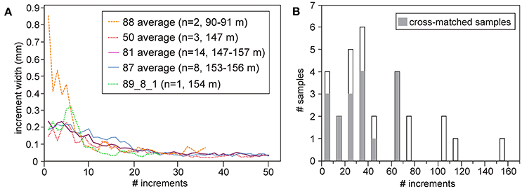
Figure 3. (A) Ontogenetic growth curves of Madeiran G. vangentsumi shells averaged by collection sites. Group 88 was collected at a depth of 90 m, while the other groups (50, 81, 87) were collected at depths between 147 and 157 m. (B) Age distribution of the 29 analyzed shells in ten-year clusters: gray filling represent successfully cross-dated shells.

Four specimens displayed <10 increments. The distribution of the counted increments shows that majority of the processed shells belonged to a range of 20–70 increments. Far fewer shells preserved more than 100 increments, of which one had 154 increments (Figure 3B).

Assessment of the Glycymeris vangetsumi Increment Chronology

Cross-matching the two live-collected shells with 14 unarticulated shells the span of the chronology was successfully extended. Based on the overlapping increment series (Figures 4A,C), a 86 increments-long composite chronology was created. Interestingly, none of the longest (>100 increments) records were cross-dated with the mean chronology. The mean interseries correlation (Rbar) ranges between ~0.4 and 0.6 without any significant difference between the H and the NE chronology (Figure 4E). The EPS reaches the 0.85 level after sample depth reaches 4 (Figures 4B,E) supporting the robustness of both composite chronologies.

FIGURE 4

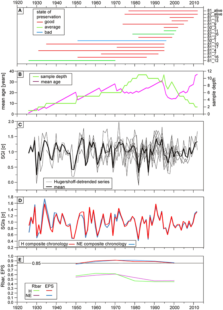
Figure 4. Details of the Madeira composite chronology from the G. vangentsumi shells. (A) Lifespan of the cross-dated shells, in which the first part of their sample code is the number of the corresponding collection site from Figure 2 color-coded by their preservation state. (B) Running mean age (purple line) and sample depth (green line) at a given time. (C) Individual Hugershoff-detrended growth increment indices (gray lines) with mean (black line). (D) Hugershoff (red line) and negative exponential (blue line) detrended (arstan) chronologies. (E) EPS and Rbar statistics of the two different chronologies calculated in 20 year running windows.

Environmental Signals and Inter-Annual Variability of G. vangentsumi Shell Growth Near the Madeira Islands

Assumed that the observed growth lines separate annual increments, calendar dates were assigned to the increments of the composite chronologies and were compared to monthly resolved time series of potentially influencing environmental parameters. A significant strong negative correlation was found between the Madeira composite increment chronology and the SST for the late winter-early spring season. The strongest significant response (r = −0.56, n = 63, p < 0.01) was identified over the period 1950–2012 between the March SST of the region (17W−16W; 33N−32N) and the two increment chronologies (Figure 5A). Significant correlations were, however, observed for the previous November to early summer, and multi-monthly means were therefore also tested. A significant correlation of similar strength was observed between the averaged November–May (r <−0.52, n = 63, p < 0.01) and January–April (r <−0.58, n = 63, p < 0.01) SST values and the two composite chronologies (Figure 5A). Spatial correlation analysis between the HadISST reconstruction and the H-detrended chronology also confirmed this relation. The March SST fields showed a significant (p < 0.05) negative correlation for the region (Figure 5B). The core area with significant correlation surrounds Madeira, covering most of the Canary Basin (Figure 5B).

FIGURE 5

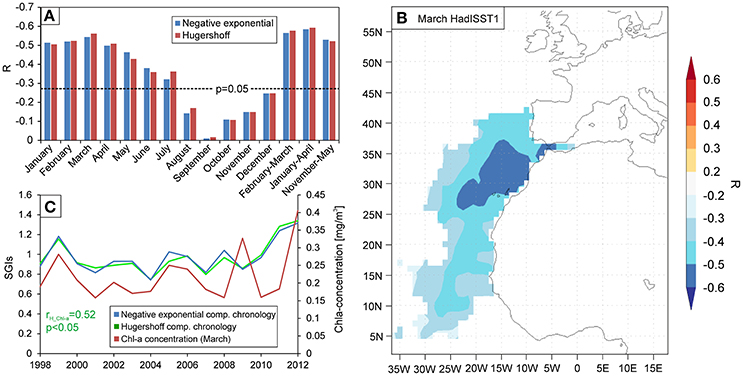
Figure 5. Correlation patterns between the shell increment chronologies and the collected environmental data of the region of Madeira. (A) Correlation coefficients calculated between the standardized increment chronologies and monthly mean sea surface temperature of the region (HadISST, Rayner et al., 2003) for the period 1950–2012. Negative exponential—detrended arstan chronology is represented by blue bars, Hugershoff -detrended arstan chronology is represented by red bars, and the dashed line corresponds to the p = 0.05 significance level. (B) Spatial correlation analysis between the gridded March HadISST field around Madeira and the Hugershoff-detrended arstan chronology calculated over the period 1950–2012. Colored areas are significant at p < 0.05 level. (C) Annual variation in March chlorophyll-a content of the surface waters of the region (red line) compared to the two chronologies between 1998 and 2012.

We observed a positive correlation (r = 0.52, n = 15, p < 0.05) between the March Chl-a concentration and the H-detrended increment chronology during 1998–2012 (Figure 5C), which is the period when Chl-a content of surface waters reaches the seasonal maximum (Martins et al., 2007). Correlation calculated between the increment chronologies and the annual mean TSI was insignificant, weak, and positive during 1950–2012.

Running correlation values (15-year windows) calculated between shell growth and monthly SST show temporal variations, however they stay significant except a short period in the beginning of the 80's (Figure 6A). Periods with warmer January–April SST, such as the 1960s and the 1990s are overlapping with periods of stronger correlation between shell growth and mean January–April SST. Correlation between shell growth and January SST was the strongest (r < −0.65) from 1967 to 1975, which also clearly overlaps with the period of the weakest correlation between shell growth and April SST (Figure 6B). Correlation between April SST is significant before 1967 and after 1988, the latter date also marks the point, where correlation between shell growth and January SST becomes insignificant (Figure 6B). Interestingly, after 1988, correlation between annual mean TSI and the H-detrended increment chronology also becomes significant.

FIGURE 6

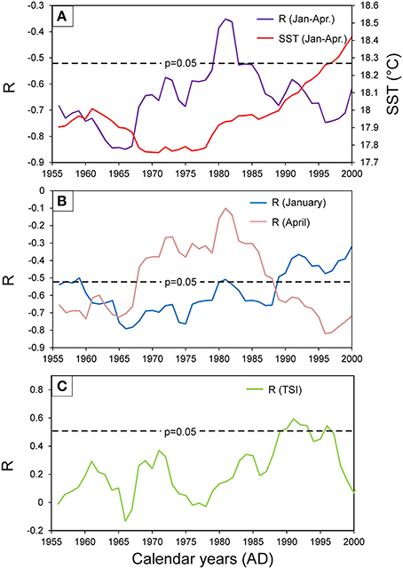
Figure 6. Temporal changes in the correlation patterns between the monthly sea surface temperature of the Madeira region (HadISST, 17W−16W; 33N−32N) and the robust section (1950–2012) of the Madeiran G. vangentsumi Hugershoff-detrended arstan chronology. Dashed lines corresponds to the p = 0.05 significance levels. (A) Correlation of the monthly averaged January–April sea surface temperature and the composite chronology (purple) calculated in 15-year running windows compared to the inter-annual fluctuations of the 15-year running mean of January–April sea surface temperature (red). (B) Coefficients of the 15-year running correlation calculated between the January sea surface temperature and the composite chronology (blue) compared to the 15-year running correlation coefficients calculated between April sea surface temperature and the composite chronology (pink). (C) Correlation calculated in 15-year running windows between the annual mean total solar irradiance and the composite chronology.

Discussion

Validation of Annual Growth Line Formation

In most cases, growth lines were easily discernible on the studied hinge plates with no thinner or fainter growth lines appearing between them, which can be a sign of regular growth cycles. Marker increments such as the thin ones labeled 1982 and 1987 and broad increments labeled as 1991, 2000, 2009, 2012 (Figure 2) were relatively easy to identify across several specimens, especially the ones with good preservation. The fact that these marker increments are cross-matching is the proof that a common environmental forcing must have affected the analyzed G. vangentsumi specimens' growth. This environmental forcing had such a strong effect on shell growth that increment series of 16 specimens collected at the same depth range (140–160 m) may be used to construct a master chronology (Figure 4) with its end point fixed, due to the known collection date of the two live-collected specimens. Annual growth line formation in Glycymeris ssp. was already validated by stable oxygen isotope analysis (e.g., Royer et al., 2013; Bušelić et al., 2015). Therefore an assumption was made that the growth of G. vangentsumi specimens from Madeira was also controlled by an annual (seasonal) environmental cycle. This hypothesis was validated by the strong and significant correlation found between seasonal SSTs, such as the averaged January–April SSTs, and the robustly cross-dated section of the composite chronology (Figure 5). By adding any yearly lag to the chronology, the correlation becomes insignificant with the aforementioned seasonal SSTs. By validating the annual growth line formation in the studied G. vangentsumi specimens, calendar dates can be assigned to the composite chronology, which is extending from 1926 to 2012.

Longevity

Generally, life spans of bivalve species are observed to be significantly shorter in the tropics than near the poles, which was explained by their faster metabolism related to better food availability (Moss et al., 2016). Consequently, the longest-lived Glycymeris spp. specimen discovered so far, a 192 years old G. glycymeris shell, was described from the Hebrides (Reynolds et al., 2013). Maximum longevities reaching 101 years (Ramsay et al., 2000) and 68 years (Brocas et al., 2013) were reported from the Irish Sea. The longest-lived G. glycymeris specimen from the Bay of Brest was only 70 years old (Featherstone et al., 2017) and from the Mediterranean no Glycymeris spp. specimen older than 65 years was described so far (Peharda et al., 2016). All aforementioned studies support the hypothesis that there is a latitudinal gradient in G. glycymeris longevity (Reynolds et al., 2013) in agreement with the same trend observed in bivalve life spans on a larger scale (Moss et al., 2016). Therefore the maximum longevity of 154 years for G. vangentsumi presented here may seem like a strong outlier considering that the samples were collected from a sub-tropical habitat. Food availability and faster metabolic rate, however, are not necessarily connected to lower latitudes as both can decrease with depth. The photic zone of the ocean surrounding Madeira is nutrient depleted through most of the year and early-spring phytoplankton blooms are less intensive than in the extra tropical Atlantic (Follows and Dutkiewicz, 2001). Probably an even smaller part of the primary production will reach the G. vangentsumi specimens' habitat at 90-160 m depth, a similar case was presented by Witbaard et al. (2003). Formation of the DCM in late-spring may also provide food for the shells (Figure 7), however, its formation is not constant in time as it depends on whether the lower boundary of the photic zone reaches the nutricline, or not (Fründt et al., 2015). The significant positive correlation found between March Chl-a surface concentration and shell growth (Figure 5C) indicates that shell growth in fact depends on food availability. Trophic constraints at the collection sites of this study are therefore probably as severe as in any high latitude habitat of Glycymeris spp., which may explain the relatively high longevity of the analyzed specimens. When conceptualizing a latitudinal trend in longevity, we also need to consider that bivalves from tropical and sub-tropical waters, especially from deeper (>100 m) environments are still under-represented in sclerochronological studies, compared to higher latitude study sites (Moss et al., 2016).

FIGURE 7

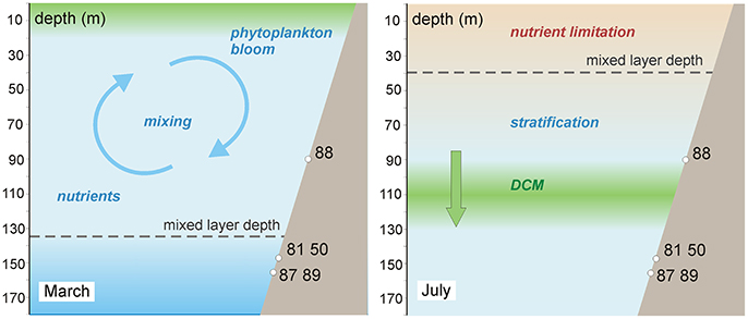
Figure 7. Schematic model of seasonal changes in environmental conditions in the G. vangentsumi shells' habitat (Madeira, Desertas Island). In early spring phytoplankton blooms are connected to high nutrient concentrations in surface waters, enhanced by ocean mixing driven by lower SST (March). Phytoplankton descend to find nutrient-rich waters as the surface becomes depleted as mixing becomes less intense. The formation of the deep chlorophyll maximum just above the shells' habitat seems favorable in terms of long-term food availability. Sea surface temperatures and mixed layer depths are based on Mason et al. (2011) while the assumed depth of deep chlorophyll maximum is based on Fründt et al. (2015).

Vertical Trend in Juvenile Growth Rates

The conspicuous difference between the ontogenetic trends of G. vangentsumi shells collected at deeper (140–160 m) and shallower (90 m) sites around Madeira (Figure 3A) indicates that the habitat depth is probably affecting juvenile growth rates. While only two samples from the shallower site were analyzed, the maximum of their averaged growth curves is at least three times higher than the maxima of averaged growth curves of any other group from the deeper collection sites. In fact, averaged increment width at the shallower site, where food availability is higher (Figure 7), remains higher during the first 8 years than in any other group (Figure 3A). Shells from collection site 88 (90 m depth) were not only living closer to the surface phytoplankton bloom, but when surface nutrient limitation forced phytoplankton species to descend to the lower part of the photic zone (90–130 m) they were situated in the depth range of DCM (Fründt et al., 2015) while food availability at the deeper sites must be even more highly seasonal (Figure 7). According with this implied vertical trend, from the Mediterranean, similarly high juvenile growth rates of G. pilosa shells from 1.5 to 3 m depth were observed (Peharda et al., 2016) to the G. vangentsumi shells collected at 90 m depth. Juvenile growth rate of shells from the 140–160 m depth range meanwhile is reduced, similarly to G. glycymeris shells collected from the Irish Sea at 37–58 m depth (Brocas et al., 2013).

Environmental Analysis

It was hypothesized in earlier studies that the link between G. glycymeris shell growth and SST can be explained by two ways: (a) they respond more directly to changes in SST because of their epifaunal lifestyle (Reynolds et al., 2013), (b) their growth is greatly affected by food availability, which often depends on SST, explaining the fact that seasonal maxima of shell growth and SST do not always coincide (Royer et al., 2013). Similarly, the strongest correlation observed between SST and a G. glycymeris increment chronology was found with the SST during the spring phytoplankton bloom rather than with the summer SST maxima (Brocas et al., 2013). In the light-limited polar and transition zones positive SST anomalies induce more intensive spring blooms, however, in the nutrient limited sub-tropical zone, this relationship is inverse (Sverdrup, 1953). In the southern regions of the North Atlantic, the mixed layer is usually shallow and irradiance is high all year round. Therefore surface waters are usually warm and depleted in nutrients (Follows and Dutkiewicz, 2001). Phytoplankton blooms can only occur if the mixed layer thickens, driven by the cooling of the sea surface in winter or early spring. In this way, the mixing process delivers nutrients into the euphotic zone, enhancing phytoplankton productivity (Mason et al., 2011). According to this, the strong and significant negative correlation observed between the G. vangentsumi chronology and the averaged January-April SST could be explained by negative correlation ascertained between the contemporaneous SST and sea surface Chl-a concentrations in the subtropical Canary Basin through the year by earlier studies (Cianca et al., 2007; Bashmachnikov et al., 2013). Phytoplankton bloom usually peaks around Madeira close to the surface at the end of February or early March (Martins et al., 2007), and these are the same months during which negative correlation is the strongest between the composite chronology and SST (Figures 5A,B). The positive correlation found between the chronology and the March Chl-a concentration of the sea surface around Madeira (Figure 5C) also supports this hypothesis. This way January–April SSTs are important environmental factors regulating the growth variability of the studied G. vangentsumi shells in an indirect way due to ocean mixing, even if the seasonal amplitude of the ambient seawater temperature in the shells' habitat is lower compared to the characteristic intra-annual fluctuation of the SST in the region (Weller et al., 2004; Mason et al., 2011). In July, surface waters warm up in the region by the mixed layer moving up to a shallower position (from 150 to ~30 m). The increased stratification is accompanied with a decrease in nutrient concentration and DCM is formed in the lower part of the photic zone (90–130 m, Figure 7), where nutrients are still available (Fründt et al., 2015). Consecutively, the strength of the correlation observed between monthly SSTs and the G. vangentsumi chronology decreases from March to July (Figure 5A).

The fact that the level of irradiance is also important for plankton growth and the formation of the DCM in the light limited zone (Fründt et al., 2015) should also be taken into account. There is increasing evidence for substantial decadal changes in the amount of solar radiation reaching the Earth's surface (“global dimming/brightening”) (Wild, 2009). Land-based observations suggest widespread declines in surface solar radiation (SSR) from the 1950s to the 1980s (“global dimming”), a partial recovery (“brightening”) since the mid-1980s (Wild, 2016). No direct observational records are available from the ocean surface. However, based on the presented conceptual ideas of SSR trends, modeling approaches, along with the available satellite-derived records, it seems plausible to suggest that over oceans similar significant decadal SSR changes have occurred (Wild, 2016). Modeling results showed that the formation of the DCM in the southern North Atlantic region ceased for several years during the so-called period of “global dimming” (Fründt et al., 2015). According to their model, from 1967 to 1973 the lower boundary of the photic zone failed to reach the nutricline, descending phytoplankton could not proliferate there after the upper layers of the photic zone had become nutrient-depleted by the beginning of summer. A DCM with lower Chl-a concentration was modeled to form until the end of 80's, when concentrations increased again.

The link between SST and shell growth in the region of Madeira can be further detailed comparing the strength of the running correlation with the January SST and the April SST, which seems to develop in opposite directions over the decades (Figure 6B). From 1967 to 1988, when DCM was modeled to reach the lowest Chl-a concentrations, the correlation coefficient between April SST and the shell-based chronology becomes non-significant, while the correlation coefficient with January SST remains significant over this period, despite the weakening correlation with the overall winter SST. These interrelations are hard to explain without further data; it seems plausible, however, that with no DCM formed during late spring-early summer, food availability in the shells' habitat became dependent solely on the intensity of the late winter ocean mixing and phytoplankton bloom, which is, in turn, determined by late winter (January) SST (c.f. Mason et al., 2011). Correlation between TSI and the H-detrended increment chronology becomes significant after 1988 (Figure 6C) simultaneously with a rapid increase in averaged January–April SST, which may indicate that formation of DCM became a more important environmental forcing parameter controlling the habitat of the bivalves near Madeira by this time.

An additional message conveyed by the information contained in Figure 6 is that short increment chronologies should be treated with caution in the quest to understand the connection between SST and shell growth, since other environmental factors varying from decade to decade may also have a great impact on the shells' habitat.

Conclusions

Here the first sclerochronological record is presented for the cockle G. vangentsumi from the subtropical region of the Atlantic Ocean. The significant longevity (up to 154 years) and the successfully synchronized growth pattern of 16 individual shells demonstrate the potential of this species for future palaeoclimate reconstruction in this location. By identifying substantial differences in juvenile growth rates at different depth ranges combined with the fact, that several 100+ years old specimens were found, this study confirms the earlier assumption that there may be not only a latitudinal, but also a vertical trend in bivalve longevity. Conversely to earlier research conducted on Glycymeris species at high latitude collection sites from the North Atlantic, in the present case the shells' growth rates are not limited by the SST; their growth, however, does reflect the early spring SST, though the causal relation is indirect. The relatively great depth of the collection sites and the high (+/−80 m) annual fluctuation of the depth of the mixing layer might be the key factors in the explanation of the significant negative correlation observed between the late-winter and early-spring SSTs and the shells' growth rates. The annual growth rate of G. vangentsumi shells from the studied population at Madeira depends more directly on the surface productivity conditioned by the upward transport of the nutrients fertilizing the photic zone, which is driven by the late-winter cooling of the sea surface and ocean mixing near Madeira. Therefore, any observed variability in the mean increment growth of G. vangentsumi shells from the ~140 to 160 m depth may be expected to serve as a prospective proxy for the inter-annual variability of the regional early spring SST. These new results may contribute to a more precise interpretation of future sub-tropical Glycymeris spp. increment chronologies.

Author Contributions

AN prepared the samples measured the data and drafted the manuscript. ZK contributed to the statistical analysis and provided input on the final version.

Funding

The research was supported by the European Union and the State of Hungary, co-financed by the European Regional Development Fund in the project of GINOP-2.3.2.-15-2016-00009 ICER.

Conflict of Interest Statement

The authors declare that the research was conducted in the absence of any commercial or financial relationships that could be construed as a potential conflict of interest.

Acknowledgments

We are grateful to the editor, Michael Hermoso and the three reviewers for their helpful and constructive comments. The authors would like to thank the CIIMAR-Madeira organization for collecting the samples analyzed in this study, Jeroen Goud for his help with the identification of the shells and the INCREMENTS Group (Johannes Gutenberg University, Mainz, Germany) where opportunity for sample preparation was provided. This is contribution No.58. of 2ka Palæoclimatology Research Group.

Supplementary Material

The Supplementary Material for this article can be found online at: https://www.frontiersin.org/articles/10.3389/feart.2018.00076/full#supplementary-material

References

Bashmachnikov, I., Belonenko, T. V., and Koldunov, A. V. (2013). Intra-annual and interannual non-stationary cycles of chlorophyll concentration in the Northeast Atlantic. Remote Sens. Environ. 137, 55–68. doi: 10.1016/j.rse.2013.05.025

CrossRef Full Text | Google Scholar

Box, G. E. P., and Jenkins, G. M. (1976). Time Series Analysis: Forecasting and Control. San Francisco, CA: Holden-Day.

Google Scholar

Brocas, W. M., Reynolds, D. J., Butler, P. G., Richardson, C. A., Scourse, J. D., Ridgway, I. D., et al. (2013). The dog cockle, Glycymeris Glycymeris (L.), a new annually resolved sclerochronological archive for the Irish Sea. Palaeogeogr. Palaeoclimatol. Palaeoecol. 373, 133–140. doi: 10.1016/j.palaeo.2012.03.030

CrossRef Full Text | Google Scholar

Buras, A. (2017). A comment on the expressed population signal. Dendrochronologia 44, 130–132. doi: 10.1016/j.dendro.2017.03.005

CrossRef Full Text | Google Scholar

Bušelić, I., Peharda, M., Reynolds, D. J., Butler, P. G., Roman Gonzalez, A., Ezgeta-Balić, D., et al. (2015). Glycymeris bimaculata (Poli, 1795) - a new sclerochronological archive for the Mediterranean? J. Sea Res. 95, 139–148. doi: 10.1016/j.seares.2014.07.011

CrossRef Full Text | Google Scholar

Butler, P. G., Wanamaker, A. D. Jr., Scourse, J. D., Richardson, C. A., and Reynolds, D. J. (2013). Variability in marine climate on the North Icelandic Shelf in a 1357-year proxy archive based on growth increments in the bivalve Arctica islandica. Palaeogeogr. Palaeoclimatol. Palaeoecol. 373, 141–151. doi: 10.1016/j.palaeo.2012.01.016

CrossRef Full Text | Google Scholar

Cianca, A., Helmke, P., Mourino, B., Rueda, M. J., Llinás, O., and Neuer, S. (2007). Decadal analysis of hydrography and in situ nutrient budgets in the western and eastern North Atlantic subtropical gyre. J. Geophys. Res. 112, C07025. doi: 10.1029/2006JC003788

CrossRef Full Text | Google Scholar

Cook, E. R. (1985). A Time Series Analysis Approach to Tree-Ring Standardization. Ph.D. dissertation, The University of Arizona, Tucson, AZ.

Cook, E. R., Briffa, K., Shiyatov, S., and Mazepa, V. (1990). “Tree-ring standardization and growth-trend estimation,” in Methods of Dendrochronology. Applications in the Environmental Sciences, eds E. Cook, and Kairiukstis L. Kluwer (Dordrecht: Academic Publishers), 104–162.

Google Scholar

Cook, E. R., and Krusic, P. J. (2007). ARSTAN – a Tree-Ring Standardization Program Based on Detrending and Autoregressive Time Series Modeling, with Interactive Graphics. Tree-Ring Laboratory, Lamont Doherty Earth Observatory of Columbia University, Palisades, NY.

Cook, E. R., and Peters, K. (1997). Calculating unbiased tree-ring indices for the study of climate and environmental change. Holocene 7, 361–370. doi: 10.1177/095968369700700314

CrossRef Full Text | Google Scholar

Featherstone, A. M., Butler, P. G., Peharda, M., Chauvaud, L., and Thébault, J. (2017). Influence of riverine input on the growth of Glycymeris glycymeris in the Bay of Brest, North-West France. PLoS ONE 12:e0189782. doi: 10.1371/journal.pone.0189782

PubMed Abstract | CrossRef Full Text | Google Scholar

Follows, M., and Dutkiewicz, S. (2001). Metreoropogical modulation of the North Atlantic spring bloom. Deep-Sea Res. II 49, 321–344. doi: 10.1016/S0967-0645(01)00105-9

CrossRef Full Text | Google Scholar

Fründt, B., Dippner, J. W., Schulz-Bull, D. E., and Waniek, J. J. (2015). Chlorophyll-a reconstruction from in-situ measurements, Part II: Marked carbon uptake decrease in the last century. J. Geophys. Res. Biogeosci. 120, 246–253. doi: 10.1002/2014JG002691.

CrossRef Full Text | Google Scholar

Fründt, B., and Waniek, J. J. (2012). Impact of the Azores front propagation on deep ocean particle flux. Cent. Eur. J. Geosci. 4, 531–544. doi: 10.2478/s13533-012-0102-2

CrossRef Full Text | Google Scholar

Goud, J., and Gulden, G. (2009). Description of a new species of Glycymeris (Bivalvia: Arcoidea) from Madeira, Selvagens and Canary Islands. Zoologische mededelingen Leiden 83, 1059–1066.

Google Scholar

Grissino-Mayer, H. D. (2001). Evaluating crossdating accuracy: a manual and tutorial for the computer program COFECHA. Tree-Ring Res. 57, 205–221.

Google Scholar

Henson, S. A., Dunne, J. P., and Sarmiento, J. L. (2009). Decadal variability in North Atlantic phytoplankton blooms. J. Geophys. Res. 114, C04013. doi: 10.1029/2008JC005139

CrossRef Full Text | Google Scholar

Holland, H. A., Schöne, B. R., Lipowsky, C., and Esper, J. (2014). Decadal climate variability of the North Sea during the last millennium reconstructed from bivalve shells (Arctica islandica). Holocene 24, 771–786. doi: 10.1177/0959683614530438

CrossRef Full Text | Google Scholar

Krivova, N. A., Vieira, L. E. A., and Solanki, S. K. (2010). Reconstruction of solar spectral irradiance since the Maunder minimum. J. Geophys. Res. 115, A12112. doi: 10.1029/2010JA015431

CrossRef Full Text | Google Scholar

Larsson, L. (2014). CooRecorder and Cdendro Programs Cybis Elektronil and Data. A. B., Sweden.

Lázaro, C., Juliano, M. F., and Fernandes, M. J. (2013). Semi-automatic determination of the azores current axis using satellite altimetry: application to the study of the current variability during 1995–2006. Adv. Space Res. 51, 2155–2170. doi: 10.1016/j.asr.2012.12.021

CrossRef Full Text | Google Scholar

Marali, S., and Schöne, B. R. (2015). Oceanographic control on shell growth of Arctica islandica (Bivalvia) in surface waters of Northeast Iceland - Implications for paleoclimate reconstructions. Palaeogeogr. Palaeoclimatol. Palaeoecol. 420, 138–149. doi: 10.1016/j.palaeo.2014.12.016

CrossRef Full Text | Google Scholar

Martins, A. M., Amorimb, A. S. B., Figueiredo, M. P., Sousa, R. J., Mendonça, A. P., Bashmachnikov, I. L., et al. (2007). “Sea Surface Temperature (AVHRR, MODIS) and Ocean Colour (MODIS) seasonal and interannual variability in the Macaronesian islands of Azores, Madeira, and Canaries,” in Remote Sensing of the Ocean, Sea Ice, and Large Water Regions Proceedings of SPIE - The International Society for Optical Engineering October 2007, eds C. R. Bostater, S. P. Mertikas, X. Neyt, and M. Vélez-Reyes (Florence: Spie), 67430A.

Google Scholar

Mason, E., Colas, F., Molemaker, J., Shchepetkin, A. F., Troupin, C., McWilliams, J. C., et al. (2011). Seasonal variability of the Canary Current: a numerical study. J. Geophys. Res. 116:C06001. doi: 10.1029/2010JC006665

CrossRef Full Text | Google Scholar

Mette, M., Wanamaker, A., Carroll, L. M., Ambrose, W. G., and Retelle, M. J. (2016). Linking large-scale climate variability with Arctica islandica shell growth and geochemistry in northern Norway. Limnol. Oceanogr. 61, 748–764. doi: 10.1002/lno.10252

CrossRef Full Text | Google Scholar

Moss, D. K., Ivany, L. C., Judd, E. J., Cummings, P. W., Bearden, C. E., Kim, W. J., et al. (2016). Lifespan, growth rate, and body size across latitude in marine bivalvia, with implications for phanerozoic evolution. Proc. Biol. Sci. 283:20161364. doi: 10.1098/rspb.2016.1364

PubMed Abstract | CrossRef Full Text | Google Scholar

Mosteller, F., and Tukey, J. W. (1977). Data Analysis and Regression: A Second Course in Statistics. Reading, MA: Addison-Wesley.

Google Scholar

NASA (2014). Sea-viewing Wide Field-of-view Sensor (SeaWiFS) Ocean Color Data. Reprocessing. NASA Goddard Space Flight Center, Ocean Ecology Laboratory, Ocean Biology Processing Group. NASA OB.DAAC, Greenbelt, MD.

Osborn, T. J., Briffa, K. R., and Jones, P. D. (1997). Adjusting variance for sample-size in tree-ring chronologies and other regional-mean time-series. Dendrochronologia 15, 89–99.

Google Scholar

Peharda, M., Black, B. A., Purroy, A., and Mihanović, H. (2016). The bivalve Glycymeris pilosa as a multidecadal environmental archive for the Adriatic and Mediterranean Seas. Mar. Environ. Res. 119, 79–87. doi: 10.1016/j.marenvres.2016.05.022

PubMed Abstract | CrossRef Full Text | Google Scholar

Peharda, M., Crncevic, M., Buselic, I., Richardson, C. A., and Ezgeta-Balic, D. (2012). Growth and longevity of Glycymeris nummaria (Linnaeus, 1758) from the eastern Adriatic. Croatia. J. Shellfish Res. 31, 940–950. doi: 10.2983/035.031.0406

CrossRef Full Text | Google Scholar

Ramsay, K., Kaiser, M. J., Richardson, C. A., Veale, L. O., and Brand, A. R. (2000). Can shell scars on dog cockles (Glycymeris glycymeris L.) be used as an indicator of fishing disturbance? J. Sea Res. 43, 167–176. doi: 10.1016/S1385-1101(00)00006-X

CrossRef Full Text | Google Scholar

Rayner, N. A., Parker, D. E., Horton, E. B., Folland, C. K., Alexander, L. V., Rowell, D. P., et al. (2003). Global analyses of sea surface temperature, sea ice, and night marine air temperature since the late nineteenth century. J. Geophys. Res. 108, D14. doi: 10.1029/2002JD002670

CrossRef Full Text | Google Scholar

Reynolds, D. J., Butler, P. G., Williams, S. M., Scourse, J. D., Richardson, C. A., Wanamaker, A. D., et al. (2013). A multiproxy reconstruction of hebridean (NW Scotland) spring sea surface temperatures between AD 1805 and 2010. Palaeogeogr. Palaeoclimatol. Palaeoecol. 386, 275–285. doi: 10.1016/j.palaeo.2013.05.029

CrossRef Full Text | Google Scholar

Richardson, C. A. (2001). “Molluscs as archives of environmental change,” in Oceanography and Marine Biology, An Annual Review, eds R. N. Gibson, M. Barnes, and R. J. A. Atkinson (London: Taylor & Francis), 103–164.

Royer, C., Thebault, J., Chauvaud, L., and Olivier, F. (2013). Structural analysis and paleoenvironmental potential of dog cockle shells (Glycymeris glycymeris) in Brittany northwest France. Palaeogeogr. Palaeoclimatol. Palaeoecol. 373, 123–132. doi: 10.1016/j.palaeo.2012.01.033

CrossRef Full Text | Google Scholar

Schöne, B. R., Dunca, E., Fiebig, J., and Pfeiffer, M. (2005). Mutvei's solution: an ideal agent for resolving microgrowth structures of biogenic carbonates. Palaeogeogr. Palaeoclimatol. Palaeoecol. 228, 149–166. doi: 10.1016/j.palaeo.2005.03.054

CrossRef Full Text | Google Scholar

Schöne, B. R., and Gillikin, D. P. (2013). Unraveling environmental histories from skeletal diaries—advances in sclerochronology. Palaeogeogr. Palaeoclimatol. Palaeoecol. 373, 1–5. doi: 10.1016/j.palaeo.2012.11.026

CrossRef Full Text | Google Scholar

Schöne, B. R., Oschmann, W., Rössler, J., Freyre Castro, A. D., Houk, S. D., Kröncke, I., et al. (2003). North Atlantic oscillation dynamics recorded in shells of a long-lived bivalve mollusk. Geology 31, 1037–1040. doi: 10.1130/G20013.1

CrossRef Full Text

Sverdrup, H. U. (1953). On conditions for the vernal blooming of phytoplankton. J. du Conseil Int. pour l'Exploration de la Mer 18, 287–295. doi: 10.1093/icesjms/18.3.287

CrossRef Full Text | Google Scholar

Teira, E., Mourino, B., Maranon, E., Perez, V., Pazo, M. J., and Serret, P. (2005). Variability of chlorophyll and primary production in the Eastern North Atlantic subtropical gyre: potential factors affecting phytoplankton activity. Deep Sea Res. I 52, 569–588. doi: 10.1016/j.dsr.2004.11.007

CrossRef Full Text | Google Scholar

Trouet, V., and Van Oldenborgh, G. J. (2013). KNMI climate explorer: a web-based research tool for high-resolution paleoclimatology. Tree Ring Res. 69, 3–13. doi: 10.3959/1536-1098-69.1.3

CrossRef Full Text | Google Scholar

Walliser, E. O., Schöne, B. R., Tütken, T., Zirkel, J., Grimm, K. I., and Pross, J. (2015). The bivalve Glycymeris planicostalis as a high-resolution paleoclimate archive for the Rupelian (Early Oligocene) of central Europe. Clim. Past 11, 653–668. doi: 10.5194/cp-11-653-2015

CrossRef Full Text | Google Scholar

Waniek, J. J., Schulz-Bull, D. E., Blanz, T., Prien, R., Oschlies, A., and Müller, T. J. (2005). Interannual variability of deep water particle flux in relation to production and lateral sources in the northeast Atlantic. Deep Sea Res I 52, 33–50. doi: 10.1016/j.dsr.2004.08.008

CrossRef Full Text | Google Scholar

Warren, W. G. (1980). On removing the growth trend from dendrochronological data. Tree Ring Bull. 40, 35–44.

Google Scholar

Weller, R. A., Furey, P. W., Spall, M. A., and Davis, R. E. (2004). The large-scale context for oceanic subduction in the Northeast Atlantic. Deep Sea Res. I Oceanogr. Res. Papers 51, 665–699. doi: 10.1016/j.dsr.2004.01.003

CrossRef Full Text | Google Scholar

Wigley, T. M. L., Briffa, K. R., and Jones, P. D. (1984). On the average value of correlated time series, with applications in dendroclimatology and hydrometeorology. J. Appl. Meteorol. Climatol. 23, 201–213.

Google Scholar

Wild, M. (2009). Global dimming and brightening: a review. J. Geophys. Res. 114, D00D16. doi: 10.1029/2008JD011470

CrossRef Full Text | Google Scholar

Wild, M. (2016). Decadal changes in radiative fluxes at land and ocean surfaces and their relevance for global warming. WIREs Clim. Change 7, 91–107. doi: 10.1002/wcc.372

CrossRef Full Text | Google Scholar

Witbaard, R., Jansma, E., and Sass Klaassen, U. (2003). Copepods link quahog growth to climate. J. Sea Res. 50, 77–83. doi: 10.1016/S1385-1101(03)00040-6

CrossRef Full Text | Google Scholar