Greenland Ice Sheet Surface Topography and Drainage Structure Controlled by the Transfer of Basal Variability

Introduction

During summer, meltwater produced on the surface of the Greenland Ice Sheet (GrIS) (van den Broeke et al., 2009; van As et al., 2012; Enderlin et al., 2014) forms a complex drainage system of streams, lakes, and moulins (Catania and Neumann, 2010; Irvine-Fynn et al., 2011; Selmes et al., 2011; Smith et al., 2015; Karlstrom and Yang, 2016; Yang and Smith, 2016). Moulins, which are surface-to-bed hydraulic connections formed by hydrofracture of surface cracks, enable meltwater to penetrate to the bed through ice more than 1 km thick in some areas (Das et al., 2008; Krawczynski et al., 2009). Such water injection raises subglacial water pressure locally, causing reduced basal friction and transient ice flow accelerations (Zwally et al., 2002; Das et al., 2008; Shepherd et al., 2009; Bartholomew et al., 2010; Sole et al., 2011; Joughin et al., 2013) which might lead to subsequent cascading hydrofracture events due to tensile shock (Christoffersen et al., 2018; Hoffman et al., 2018). However, subglacial channel expansion by wall melt can increase drainage system efficiency over a melt season, so that increased surface melt on annual-to-decadal timescales could result in a net ice flow deceleration near the ice sheet margins (van de Wal et al., 2008; Sole et al., 2013; Tedstone et al., 2015). Despite these advancements in understanding, the net long-term influence (10² years and longer) of hydrology on ice dynamics in a warming climate remains uncertain, because existing observations of the mechanism cover a relatively short time period (< 20 years) and the above processes are yet to be incorporated in a robust manner into ice sheet models (IPCC, 2013; Flowers, 2015).

The surface drainage structure of the GrIS (i.e., the distribution, density, and dimensions of lakes, streams, and moulins) controls the location and characteristics of the surface-to-bed meltwater connections (Selmes et al., 2011; Kingslake et al., 2015; Smith et al., 2015; Ignéczi et al., 2016; Yang and Smith, 2016). Therefore, understanding the factors that control this structure is a prerequisite for evaluating the long-term effects of hydrological processes on ice sheet dynamics. Meltwater production and runoff depends on atmospheric and ice-surface conditions, including temperature, irradiation, precipitation, firn layer thickness, surface permeability, and albedo (Lüthje et al., 2006; Leeson et al., 2012; Poinar et al., 2017). The large-scale surface drainage structure is primarily determined by ice surface topography (Lüthje et al., 2006; Banwell et al., 2012; Leeson et al., 2012; Ignéczi et al., 2016; Karlstrom and Yang, 2016), which, on length-scales comparable to the ice thickness (mesoscale), is influenced by basal topography and slipperiness variability (Gudmundsson, 2003; Raymond and Gudmundsson, 2005; Ng et al., 2018).

Surface lakes, major surface streams and moulins have been observed to re-occur in approximately the same location from year to year, instead of advecting with ice flow (Echelmeyer et al., 1991; Catania and Neumann, 2010; Selmes et al., 2011). Furthermore, surface drainage basins and surface meltwater flux have been shown to correlate with basal topography (Karlstrom and Yang, 2016). These observations support the idea that ice-surface topographical features can be fixed in space by the bed topography at scales relevant to the routing of surface water. The key mechanism is that ice flow can cause basal variability to be “transferred” or “transmitted” upward to perturb the surface topography (Gudmundsson, 2003). However, to date, empirical tests of this transfer theory in the context of surface drainage have been spatially limited (Lampkin and Vanderberg, 2011) and have not utilized the theory to predict surface topography or drainage structures.

In this paper we use a recent advance made in calculating mesoscale surface topographical undulation profiles generated by the bed-to-surface variability transfer (Ng et al., 2018), together with new high-resolution bed and surface DEMs for the GrIS (Howat et al., 2014, 2017; Morlighem et al., 2017b), to conduct ice sheet-wide surface relief (i.e., topographical variability of the ice sheet surface derived from the amplitudes of mesoscale surface topographical undulation profiles) prediction experiments. We test the predicted surface relief against the observed surface relief and assess the errors associated with the predictions. We also explore to what extent the bed-to-surface variability transfer, through its control on ice surface relief, preconditions the large-scale spatial structure of surface drainage. In doing so, our study extends the framework of the bed-to-surface variability transfer theory to evaluate the long-term effects of surface drainage on ice sheet dynamics.

Methods

Predicting Surface Topographical Variability

The transfer of variability in basal topography and slipperiness to the surface (Figure 1A) has been mathematically expressed for a parallel, plane-slab ice flow with isotropic rheology and constant viscosity (Gudmundsson, 2003). A new extension of calculating this transfer, based on non-stationary convolution and applicable to 2D (i.e., a 1D flowline of varying ice thickness) flow sections (Ng et al., 2018), allows us to estimate the topographical response of the surface to basal perturbations (to both topography and slipperiness) when background variables (ice thickness, surface slope, and basal slip ratio: sliding velocity/deformational velocity) vary with distance x along individual flowlines. Specifically, if b(x) and c(x) represent the basal topography and slipperiness perturbations, respectively, then the Fourier transform of the surface elevation response is given by

$\begin{array}{l}ŝ(k)={\displaystyle {\int }_{-\infty }^{\infty }}{T}_{sb}(k,x)b(x)e^{-ikx}dx\\ +{\displaystyle {\int }_{-\infty }^{\infty }}{T}_{sc}(k,x)c(x)H(x)e^{-ikx}dx& (1)\end{array}$

(Ng et al., 2018), where k denotes wavenumber, H(x) is the background ice thickness and the transfer functions T_sb and T_sc (reported by Gudmundsson, 2003) vary with the background variables and thus depend on x. The surface response s(x), itself a perturbation superimposed on the background surface elevation profile, is found by computing the inverse Fourier transform of ŝ:

$\begin{array}{ll}s(x)=\frac{1}{2\pi }{\displaystyle {\int }_{-\infty }^{\infty }}ŝ(k)e^{ikx}dk.& (2)\end{array}$

As flowlines have finite lengths, the integrals are evaluated as discrete sums in the same way as in the Discrete Fourier Transform and its inverse (Ng et al., 2018). In the calculations of the transfer, reported below, we use the particular forms of T_sb and T_sc given by section 4.9 of Gudmundsson (2003), which were derived from a linearised ice-flow theory assuming constant ice viscosity.

FIGURE 1

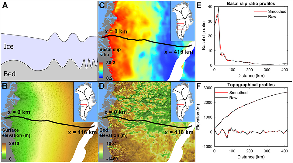
Figure 1. (A) Cartoon illustrating the transfer of basal topographical variability (perturbations) to the ice surface. Ice flow behaves as a filter preferentially transferring bed topographical undulations of particular wavelengths compared to the ice thickness. (B) Maps of ice surface topography, (C) basal slip ratio (D) and bed topography in SW Greenland, showing a sample flowline (bold curve). (E) Raw profiles of basal slip ratio, (F) bed and surface elevations derived from the map along the flowline, and their corresponding smoothed versions. Areas around the ice divides are masked out to minimize edge effects.

Ice flowlines were derived from a modeled ice surface velocity field of the contemporary GrIS (Price et al., 2017). Their tracing required manually delineating 5,138 seed points close to the ice divides, to ensure an adequate density of lines for the whole ice sheet. Along each flowline, surface topography, bed topography, and basal slip ratio, were sampled at a spacing of 250 m (Figure 1). Surface topography was obtained from the MEaSUREs Greenland Ice Mapping Project (GIMP) DEM from GeoEye and WorldView Imagery, Version 1 dataset (Howat et al., 2014, 2017; 30 m grid resolution), bed topography from the IceBridge BedMachine Greenland, Version 3 dataset (Morlighem et al., 2017a,b; 150 m grid resolution), and basal slip ratio from a dataset by MacGregor et al. (2016). The final basal slip dataset, calculated by the formula u_s/u_d (u_s: representative surface velocity, u_d: deformational velocity), generally underestimates true basal slip ratios due to overestimation of the u_d and underestimation of u_s. The overestimation arises from the assumption of fully temperate ice throughout the GrIS, and the underestimation arises from the use of observed winter ice flow velocity to represent annual ice motion, which ignores summer speed-up events (Bartholomew et al., 2010). We conducted sensitivity experiments to assess the effects of u_d overestimation (detailed in Supplementary Material 1) and u_s underestimation (detailed in section Prediction of the Mean Surface Relief) on our surface relief predictions.

Bed topography, ice-surface topography and basal slip ratio profiles (Figures 1E,F) were smoothed using a 6th-order Butterworth low pass filter to separate background variables (smoothed data) which determine the strength of the transfer (Figures 2A–C), and basal perturbations (raw minus smoothed data) which are transferred to the surface (Figure 2D). While this subtraction for the bed elevation yielded b(x) directly (Figure 2D), the slipperiness forcing c(x)—defined in the transfer theory as mesoscale perturbations on the coefficient of the basal sliding law (Gudmundsson et al., 1998; Gudmundsson, 2003)—is unknown, because direct observations/measurements of subglacial properties are lacking. One way of estimating c(x) is to treat the ice flow as an inverse problem for constraining the basal conditions, using knowledge of u_s and the surface topographical undulations as inputs (discussion by Ng et al., 2018), but this difficult problem is not tackled by us here. Note that this issue with c(x) does not concern the background slip ratios conditioning the transfer (De Rydt et al., 2013), which are simply derived as the smoothed version of the basal slip ratio dataset. Although c(x) is unknown, theory suggests that its effect on surface topographical undulations may be small compared to b(x) (Gudmundsson, 2003; De Rydt et al., 2013) in many areas (unless b(x) ≈ 0, on ice streams with exceedingly smooth beds). Hence, here we neglected the second integral of Equation (1), containing c(x), in our calculations but nevertheless undertook experiments to assess its potential effects on the surface topography (Supplementary Material 2). The observed ice-surface undulations, defined by the perturbation s(x) (Figure 2E), were derived by subtracting the smoothed surface topographical profile from its raw version. To predict s(x) (Figure 2E), we carried out the integral method in Equations (1) and (2), using the basal topographical perturbation profiles b(x) and the background profiles as the inputs.

FIGURE 2

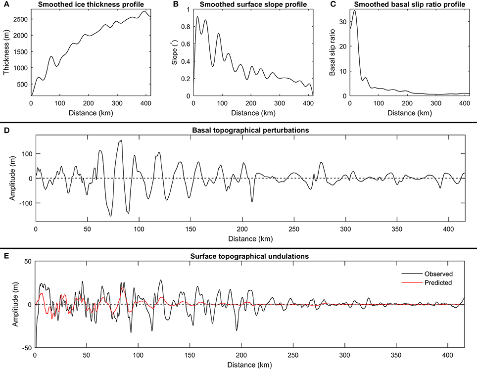
Figure 2. Prediction experiment with the flowline in Figure 1. Background variables: (A) ice thickness, (B) ice-surface slope, (C) basal slip ratio, (D) and basal topographical perturbations. (E) Observed and predicted surface topographical undulations, showing correspondence between some of their peaks and troughs.

As the linearised transfer theory of Gudmundsson (2003) was derived for a parallel slab flow, the smoothing distance in the Butterworth filter, which determines its corner frequency, should reach or exceed the length-scale at which the shallow-ice approximation applies (~10 times the regional ice thickness). We experimented with a range of smoothing distances, from 5 to 30 km, in steps of 5 km (Supplementary Material 3). Greater smoothing distances enabled the inclusion of longer surface undulations in the transfer and dampened fast spatial changes in the background variables, ensuring that the approximations behind the use of non-stationary convolution in Equation (1) are applicable (Ng et al., 2018). But greater smoothing distances retained larger amplitude perturbations, which can invalidate the approximations behind Gudmundsson's (2003) linearized transfer theory (Ng et al., 2018). In our GrIS exploration, a smoothing distance of 20 km was found to be near-optimal in satisfying both conditions as far as possible (Supplementary Material 3), and was therefore used in the rest of the paper. This choice matches the requirement that the smoothing distance exceeds 10 times the mean ice thickness (1,632 m) along our flowlines.

A continuous wavelet transform (CWT—Equation 3) was applied to the observed and predicted surface topographical undulation profiles to study their spectral composition (Figure 3):

$\begin{array}{ll}{W}_f(p,a)={\displaystyle {\int }_{-\infty }^{\infty }}f(x)\frac{1}{\sqrt{a}}{\text{Ψ}}^{*}\left(\frac{x-p}{a}\right)dx& (3)\end{array}$

Here f (x) is the observed or predicted surface undulation profile, p is the position, a is the scale, Ψ is the mother wavelet for which an analytic Morlet wavelet was chosen (ω₀ = 6), and * represents the complex conjugate (Mallat, 2009; Alessio, 2016). The absolute value of the real part of the continuous wavelet transforms measures the amplitudes of surface undulations at wavelengths below the smoothing distance (Figure 3). Subtracting the observed CWT amplitudes from the predicted CWT amplitudes gives an “anomaly” (Figure 3C) that reveals any under- and over-estimation of the amplitude of surface undulations at different wavelengths and positions. Detailed analysis of all CWT and anomaly plots for our several thousand flowlines across the GrIS was not feasible. Instead, for each flowline, we condensed the plots by averaging their results over the mesoscale range of wavelengths (up to the smoothing distance) to create spatial profiles of observed mean surface undulation amplitude, predicted mean surface undulation amplitude, and mean amplitude anomaly (Figures 3D–F). For brevity, these are henceforth referred to as observed/predicted mean surface relief and relief anomaly. Linear regression was applied to test the expected 1:1 linear relationship between the observed and predicted mean surface relief along all flowlines simultaneously, testing the overall performance of our method. Color-coded maps of the whole ice sheet were also produced from the observed/predicted mean surface relief and relief anomaly profiles by kriging interpolation, for visual inspection of spatial patterns. Although maps could also have been made directly from the observed and predicted surface topographical undulation profiles (Figure 2F), their repeated zero crossings would have complicated the spatial analyses. Our approach circumvents this problem by first extracting amplitudes in spectral terms.

FIGURE 3

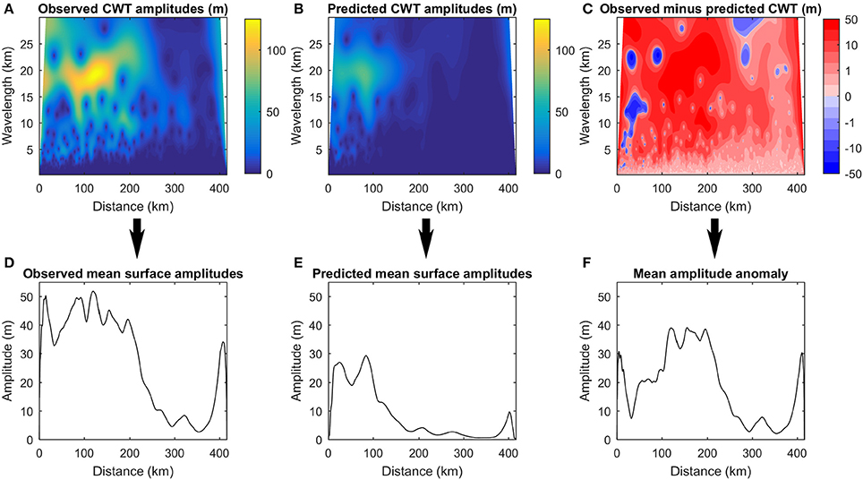
Figure 3. (A) Continuous wavelet transforms (CWT) of the observed (B) and predicted surface undulation profiles along the flowline in Figure 1. In these “scalograms,” CWT amplitude measures the strength of variability (thus, undulation amplitude) of different wavelengths at different positions. (C) Amplitude difference between (A,B) is also shown. The lower plots, made by averaging the upper plots over different wavelengths, quantify the (D) observed (E) and predicted mean mesoscale surface undulation amplitudes (F) and the mean amplitude anomaly along the flowline.

Surface Streams and Lakes, Closed Surface Depressions, Moulins, and Principal Strain Rates

To evaluate the influence of the bed-to-surface variability transfer on the surface drainage structure of the GrIS, we compared the observed and predicted mean surface relief with the observed distribution of surface lakes, surface rivers and moulins. These features were derived from Landsat-8 panchromatic imagery, with 15 m horizontal resolution, acquired on 19 August 2013, for a 22,788 km² area in SW Greenland (Yang and Smith, 2016). In order to control for the influence of surface meltwater runoff on the distribution of surface drainage features derived from Landsat-8 imagery, modeled monthly runoff data from Modèle Atmosphérique Régional (MAR, version 3.5.2; 5 km grid resolution), forced by European Centre for Medium Range Weather Forecast Re-analysis (ERA-Interim), were obtained for August, 2013 (Fettweis et al., 2017).

The Landsat-8 derived datasets of Yang and Smith (2016) only provide a 1 day snapshot of the temporal evolution of the surface drainage in SW Greenland. However, in reality, surface drainage evolves in time as the meltwater production varies across the GrIS, governed by changing atmospheric conditions and surface energy balance (Yang and Smith, 2016). We therefore also estimated the maximal potential distribution of lakes, rivers, and moulins by delineating closed surface depressions, surface rivers, and moulins from surface DEMs that overlap with the domain of the Landsat-8 survey. Closed surface depressions, which represent potential sites for surface lake formation, were extracted from the GIMP-DEM (Howat et al., 2014, 2017) following the approach of Ignéczi et al. (2016). Surface streams were also delineated from the GIMP-DEM using standard hydrologic analysis tools in ArcGIS. A minimal catchment area of 0.3 km² was used for river delineation, which provided the best match with observed rivers derived from Landsat-8 imagery (Supplementary Material 4). As moulins are hard to detect on moderate resolution surface DEMs, they were mapped manually using a Surface Extraction with TIN-based Search-space Minimization (SETSM) DEM (Noh and Howat, 2015; 2 m grid resolution), which is available for a 14,576 km² area in SW Greenland, largely overlapping with the Landsat-8 domain.

Crucially, these datasets, with the exception of the SETSM-DEM derived moulin survey, allow us to carry out ice sheet-wide investigations on observed/predicted surface relief and potential surface lake and river sites, even where the formation of such drainage features is inhibited due to current atmospheric conditions (e.g., in the interior of the GrIS where surface runoff is currently negligible). In order to overcome the spatial limitations of our SETSM-DEM derived moulin survey, an ice sheet-wide principal strain rate map was also derived from a mean of MEaSUREs ice flow velocity datasets (Version 2) for the winters of 2007–2009 (Joughin et al., 2010, 2017) following the approach of Poinar et al. (2015). The formation of moulins due to hydrofracture requires an initial crack (e.g., a crevasse) at the ice sheet surface, which is propagated to the ice sheet bed by tensile stresses due to meltwater infilling (Das et al., 2008; Krawczynski et al., 2009). The spatial distribution of crevasses has been shown to correspond well with areas of principal strain rates above +0.005 yr⁻¹ (Joughin et al., 2013; Poinar et al., 2015). Our principal strain rate map thus allows a first order investigation of the connection between surface relief and potential sites for hydrofracture at the ice sheet scale.

Results and Discussion

Prediction of the Mean Surface Relief

Generally, and as expected, the observed mean surface relief decreases toward the interior of the GrIS, though the rate of decrease shows significant regional differences (Figure 4A). Large surface relief is found extending far from the ice sheet margin in the W, NW and NE catchments of the GrIS (Figure 4A) (e.g., on the upstream part of Jakobshavn Isbrae and on the Northeast Greenland Ice Stream), where we see deep inland penetration of high basal topographical variability (Figure 4C) and high basal slip ratios (Rippin, 2013; MacGregor et al., 2016; Figure 4D). In contrast, in the N, E and SW catchments, where such inland penetration is limited (Figures 4C,D), the observed mean surface relief decays quickly away from the margin (Figure 4A). These correlations confirm the theoretical expectation that the transfer of basal topographical variability to the surface is attenuated by thicker ice and lower ice surface slopes, and high basal slip ratio enables more efficient transfer (Gudmundsson, 2003; Raymond and Gudmundsson, 2005). The visible spatial correlation between the predicted and observed mean surface relief (Figures 4A,B) also confirms the qualitative explanatory power of Gudmundsson's (2003) theory.

FIGURE 4

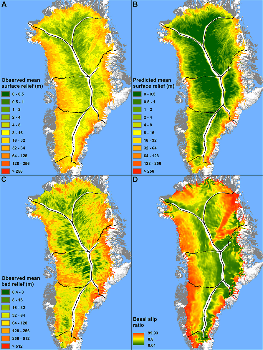
Figure 4. (A) Maps of observed mean ice-surface relief, (B) predicted mean ice-surface relief, (C) observed mean bed relief (D) and basal slip ratio across the GrIS. Areas around the ice sheet divides are masked out to minimize edge effects.

According to the transfer functions T_sb and T_sc, across the GrIS the surface topographical response to basal slipperiness perturbations is significantly weaker than the response to basal topographical perturbations at the wavelengths investigated here (Gudmundsson, 2003; De Rydt et al., 2013; Ng et al., 2018). In other words, the surface topographical relief is controlled predominantly by basal topographical perturbations, i.e., via T_sb in Equation (1), while the ice thickness, basal slip ratio, and surface slope modulate this control. This theoretical expectation is confirmed by our sensitivity experiments assuming basal topography and slipperiness perturbations of the same magnitude (Supplementary Material 2). These demonstrate that the relative mean surface relief response to basal slipperiness perturbations—compared to the total surface relief response—is below 25% for typical GrIS conditions today (Supplementary Material 2).

We proceeded to quantify the performance of the method outlined in Equations (1) and (2) in capturing the transfer, whose explanatory power has already been attested by visible correlation between the observed and predicted mean surface relief maps (Figures 4A,B). Linear regression demonstrates a statistically significant (p < 0.01) relationship between these relief variables (Figure 5), with the best-fit equation (slope = 1.13; intercept = −8.64) deviating slightly from perfect match (slope = 1; intercept = 0). Despite this impressive result and the spatial correlation (Figures 4A,B), which indicate general success of the method, there is a considerable mean absolute error (14.9 m) between the observed and the predicted mean surface relief. Additional insights come from the map of relief anomaly (i.e., spectral-mean difference between observed and predicted CWT amplitudes), which reveals systematic patterns in the amount of underestimation (positive anomaly) or overestimation (negative anomaly) of the predictions across Greenland (Figure 6B). The frequency distribution of the relief anomaly is bi-modal, with one modus at +8 m and another at −16 m (Figure 6C). Most of the ice sheet (92.5%) is characterized by underestimation, while overestimation is restricted to numerous small areas close to the margins (Figures 6A,C). These negative anomalies often correspond with the high absolute principal strain rates on fast-flowing outlet glaciers (Figures 6C–E,G,H).

FIGURE 5

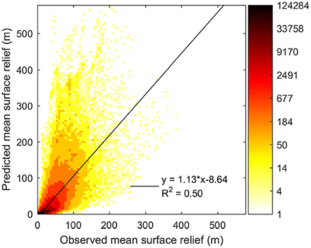
Figure 5. Predicted mean surface relief against observed mean surface relief calculated along our flowlines (before interpolation), on a data density plot. The color bar indicates the number of data points per pixel.

FIGURE 6

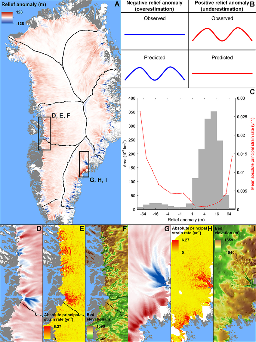
Figure 6. (A) Map of surface relief anomaly across the GrIS. (B) Cartoon of surface topography explaining what the two types of relief anomaly. The anomaly is negative (blue) where the observed relief is less than predicted, and positive (red) where it is more than predicted. (C) Ice sheet-wide frequency distribution of relief anomalies and the corresponding means of the absolute principal strain rates, categories smaller than 4,500 km² have been removed and accordingly the color scale was capped on (A). (D,G) Relief anomaly, (E,H) absolute principal strain rate (F,I), and bed topography in the two regions outlined by the boxes in (A).

Several reasons may explain the overall mismatch between the predicted and observed surface relief, and the spatial pattern of the relief anomaly. Firstly, our method is based exclusively on the transfer theory, thus other surface relief production processes are not incorporated. For example, redistribution of the snow/firn coverage on the ice sheet surface by strong winds can cause sastrugi to form. However, these are transient and have relatively small amplitude and wavelength, thus they only mildly increase the surface relief (Whillans, 1975). Surface processes, such as spatial variations in surface mass balance and snow/firn compaction rates, can also modify the shape of larger surface topographical undulations. However, these processes are unlikely to affect the position and phase of the undulations significantly (Black and Budd, 1964; Gow and Rowland, 1965; Whillans, 1975; Medley et al., 2015). Hence, we propose that surface processes only exert a secondary feedback on the magnitude of surface relief. This is supported by the fact that we can predict the pattern of surface relief well without incorporating their effects.

Some of the mismatch between predicted and observed surface relief is attributable to underestimation of the true basal slip ratios by our basal slip ratio dataset. This would cause an underestimation of the surface relief, as faster basal slip promotes efficient transfer of basal variability (Gudmundsson, 2003); indeed, most of the ice sheet is characterized by positive relief anomalies (Figure 6). Two sensitivity tests were carried out to quantify how much basal slip ratios may have been underestimated due to (i) their derivation from winter surface velocities (which exclude summer speed-up events) and (ii) the assumption by MacGregor et al. (2016) of a fully temperate ice column across the GrIS (both explained in section Predicting Surface Topographical Variability), and the consequences for our outputs. In the first test, basal slip ratios were re-calculated using the deformational velocities provided by MacGregor et al. (2016) and observed annual surface velocities derived from feature tracking of Landsat 8 images acquired on 6th August 2014 and 25th August 2015 over a 4,205 km² area in SW Greenland (Figure 7). This new basal slip ratio dataset was then used to re-predict the surface relief again of this area. Comparison of the new prediction against the original prediction shows that the use of winter velocities (thus, neglecting summer ice flow speed-ups) in the original caused a significant underestimation of basal slip ratios across the area (Figure 7A), but only a moderate underestimation of the predicted surface relief (Figure 7B). The second sensitivity test, exploring the assumption of a fully temperate ice column across the GrIS by MacGregor et al. (2016), is detailed in Supplementary Material 1. It shows that this assumption raises the rate of inland decrease of the predicted surface relief across the GrIS, but the large-scale spatial pattern of our standard prediction is robust.

FIGURE 7

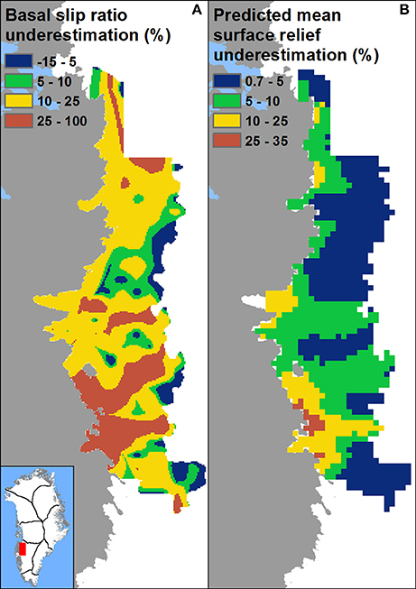
Figure 7. (A) The percentage of the basal slip ratio underestimation caused by the usage of winter, instead of annual, ice flow velocities, (B) the underestimation of the predicted mean surface relief caused by the usage of winter, instead of annual, basal slip ratios.

A further potential cause of the systematic spatial pattern of over—and underestimation of surface relief is the assumption of constant viscosity—exhibiting a linear stress-strain relationship (i.e., linearly viscous medium)—in our transfer calculation (Gudmundsson, 2003; Ng et al., 2018). Where strain rates are high, the ice viscosity decreases according to Glen's flow law (Figure 8). The attendant faster internal deformation would more strongly attenuate the upward transfer of basal perturbations, causing a smoother surface than predicted. This hypothesis is supported by the correspondence of negative relief anomalies with high strain rate magnitudes, mostly in the vicinity of high velocity outlet glaciers (Figure 6). Where strain rates are low, more rigid ice than assumed (Figure 8) would act as a stress guide to cause stronger transfer (Raymond and Gudmundsson, 2005). This expectation is consistent with the dominance of positive anomalies in the ice sheet interior (Figure 6). However, such nonlinear rheological effects mainly change the quantitative strength of the bed-to-surface transfer, not its qualitative behavior (Raymond and Gudmundsson, 2005). This is supported by the overall correlation between the observed relief map and our predicted map.

FIGURE 8

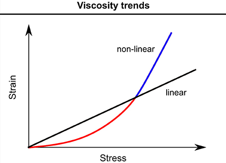
Figure 8. Stress-strain graphs of a linearly viscous medium, assumed in our calculations, and a non-linearly viscous shear-thinning medium, which is a more precise representation of glacier ice, are shown. Negative relief anomalies (blue) are suggested to correspond with areas where the linear approximation overestimates viscosity, at high stress-strain rates, and vice versa (red).

Other factors responsible for the relief anomalies are unknown basal slipperiness perturbations, bed DEM uncertainty, 3D effects on the transfer of basal variability and the presence of deeply incised subglacial valleys. By omitting basal slipperiness perturbations from the transfer function we anticipate some underestimation of the mean surface relief, although this is expected to be small (< 25%) and become less significant under thicker ice (Supplementary Material 2). The BedMachine mass conservation algorithm is less precise (Morlighem et al., 2014, 2017b) and basal topographical features could be missed (Ross et al., 2018), where the spatial density of ice thickness measurements is low. Our method will under-predict the amplitude of surface undulations in such data-sparse regions. Accordingly, we observe the dominance of positive relief anomalies in the GrIS interior (Figure 6) where ice thickness measurements are scarce (Morlighem et al., 2014, 2017b). Also De Rydt et al. (2013) demonstrated that the 3D transfer of basal variability is weaker than described by the 2D approximations along flowlines. This “dampening” effect, which would induce negative relief anomalies in our predictions, is expected to be significant around laterally-confined ice flow features that show strong lateral variations in basal properties (De Rydt et al., 2013; Sergienko, 2013). The effect is evidenced by the frequent alignment of deeply incised subglacial valleys with our computed negative relief anomalies, e.g., the Jakobshavn Glacier in W Greenland and the Helheim Glacier in the SE (Figures 6D–I). The latter site is especially interesting, as strongly positive amplitude anomalies aligned with high strain rates and a disconnected system of subglacial depressions are found directly inland of deep fjords along the ice sheet margin (Figures 6G–I). We propose that areas such as this have poorly resolved bed topography and as yet undiscovered major subglacial valleys.

Surface Topographical Control on Contemporary Surface Drainage Structure

Here, we test the hypothesis that bed-to-surface variability transfer controls the spatial pattern of surface drainage at the ice sheet scale. This is crucial as it enables us to use the predicted mean surface relief—obtained by employing the theory of bed-to-surface variability transfer—as a proxy for estimating palaeo/future surface drainage structures. Comparing the predicted mean surface relief and the surface drainage is the most direct way of doing this. However, mismatches between the observed and predicted mean surface relief—due to known limitations of the theory and the input data—will bias these relationships. Hence, we also compare the surface drainage with the observed mean surface relief, which has been shown to be controlled by the bed-to-surface variability transfer in section Prediction of the Mean Surface Relief. This approach allows us to circumvent the bias and provides flexibility for palaeo/future predictions where data uncertainties (e.g., knowledge of bed) will vary.

Observed Mean Surface Relief and Surface Drainage

The spatial density of Landsat-8 derived surface lakes and GIMP-DEM derived closed surface depressions in SW Greenland (Figure 9) is highest in areas displaying moderate observed surface relief, around 25 m (Figure 9D). This result is found also for the subsets of the Landsat-8 lakes corresponding to different runoff intervals (Figure 9D) though the 100–300 mm interval lacks relief exceeding 32 m (Figure 9C). Despite the very similar trend to Landsat-8 derived lakes, GIMP-DEM derived depressions have a higher overall areal coverage than Landsat-8 derived lakes. This is expected because the topographic depressions delineate the maximal potential lake coverage (Ignéczi et al., 2016), whereas the Landsat-8 time snapshot records actual lakes in existence on 19 Aug 2013. The runoff interval subsets indicate that the overall lake coverage decreases with higher runoff (Figure 9D). A likely reason is that the Landsat-8 snapshot was acquired late in the melt-season when many lakes at lower elevations, where the runoff is higher, had already drained (Sundal et al., 2009). In the context of the null hypothesis, that these features are randomly distributed in relation to the surface relief, the maximal standard score (maximum standardized deviation from the mean) of the areal coverage of lakes is statistically significant for the full Landsat-8 domain (Table 1). Depressions and subsets of lakes for different runoff categories yielded similar, albeit statistically less significant, results (Table 1). These results indicate a strong control on surface lake and depression structure by the surface relief, somewhat biased by runoff.

FIGURE 9

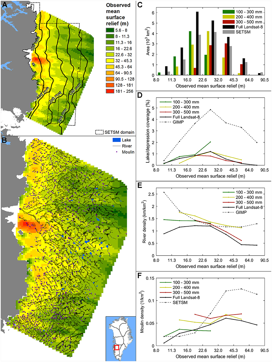
Figure 9. (A) Observed mean surface relief map for the full Landsat-8 survey domain combined with the outlines of the SETSM domain (dashed boundary) and contours representing different levels of the modeled Aug, 2013 runoff. (B) Observed mean surface relief compared with the distribution of Landsat-8 derived surface lakes, rivers and moulins in SW Greenland. (C) Area histograms of the observed mean surface relief categories of the full Landsat-8 domain, SETSM domain, and different runoff intervals of the Landsat-8 domain; categories smaller than 160 km² and in the case of the SETSM domain above the relief of 90.5 m are excluded. (D) Landsat-8 derived lake coverage and GIMP-DEM derived depression coverage, (E) Landsat-8 and GIMP-DEM derived river density, (F) Landsat-8 and SETSM-DEM derived moulin density corresponding to observed mean surface relief categories. (D–F) To control for runoff, subsets of Landsat-8 derived lakes, rivers and moulins were created for the runoff intervals of 100–300, 200–400, and 300–500 mm.

TABLE 1

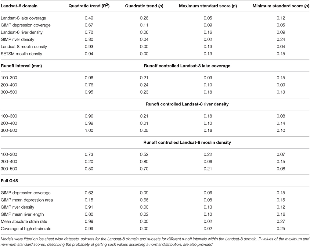
Table 1. Coefficients of determination (R²) and p-values of the quadratic models fitted on different inferential characteristics (e.g., density, coverage) of our Landsat-8, GIMP-DEM, and SETSM-DEM derived surface drainage features, principal strain rates and observed mean surface relief.

Landsat-8 derived rivers for the full Landsat-8 domain also have their highest spatial density in areas with moderate surface relief (Figure 9E), though the corresponding maximal standard score has a relatively low statistical significance (Table 1). This relationship is less clear when we consider GIMP-DEM derived rivers and Landsat-8 derived river subsets for different runoff intervals (Figure 9E), all of which suggest that the density of rivers generally decrease with increasing surface relief (Figure 9E). These decreasing trends are described by statistically significant quadratic equations except for the low runoff subset (Table 1). This limited coherence between the different trends suggests additional controlling factors besides surface relief.

Moulin density extracted from the Landsat-8 image and the SETSM-DEM increases with surface relief (Figure 9F). The SETSM-DEM reveals a higher overall moulin density, which is not surprising given its time-integrated nature and higher spatial resolution (Figure 9F). Both trends can be described by statistically significant quadratic equations (Table 1). Landsat-8 derived moulin densities in areas belonging to the different runoff intervals exhibit statistically insignificant increasing trends with surface relief (Figure 9F) and are offset from each other, implying that moulin density increases with runoff.

The ice sheet wide distribution of GIMP-DEM derived surface depressions has the highest areal coverage around moderately high surface relief (Figure 10E), while depressions are largest around moderately low surface relief (Figure 10F). Maximal standard scores of the depression coverage and mean depression area have statistical significance levels just above the conventional 0.05 boundary (Table 1). The ice sheet wide density and mean length of the GIMP-DEM derived surface rivers decrease with increasing surface relief, following statistically significant quadratic equations (Figures 10G,H, Table 1). Absolute principal strain rates and the coverage of principal strain rates above +0.005 yr⁻¹, which could be considered a proxy for crevasses and moulins (Poinar et al., 2015), increase monotonically with observed surface relief (Figures 10I,J) following quadratic equations (Table 1). These results, approximating the relationship between observed surface relief and the maximal potential ice sheet wide surface drainage, resemble the relationships observed in SW Greenland.

FIGURE 10

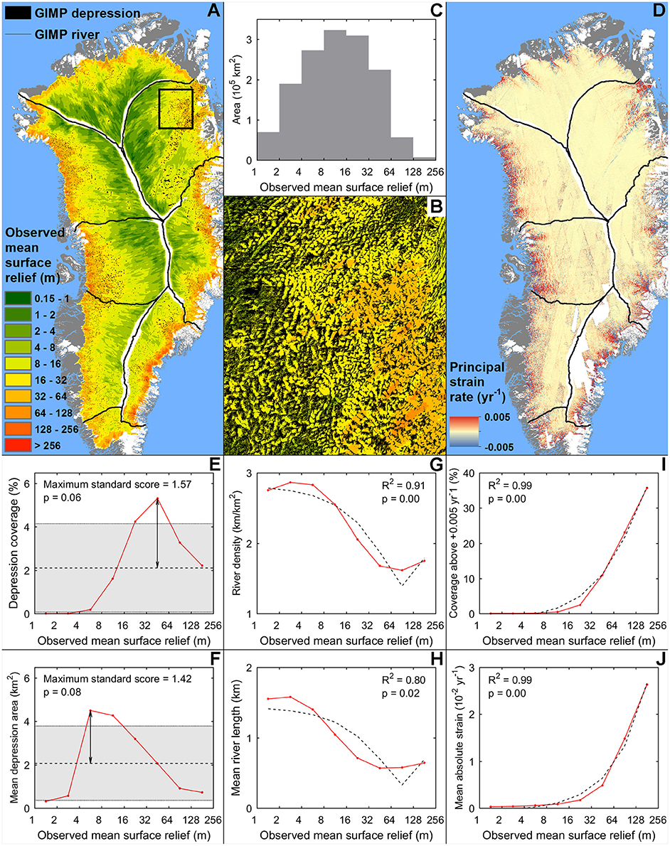
Figure 10. (A) Observed mean surface relief map compared with the distribution of GIMP-DEM derived closed surface depressions of the whole ice sheet (B) and GIMP-DEM derived rivers of NE Greenland. (C) Area covered by the observed mean surface relief categories of the GrIS is also shown; categories smaller than 4,500 km² have been removed. (D) The ice sheet wide principal strain rate is also shown. (E) The coverage (F) and mean area of the GIMP-DEM derived depressions corresponding to observed mean surface relief categories has been calculated from the ice sheet wide depression dataset. (G) The density (H) and mean length of the GIMP-DEM derived rivers, (I) the mean absolute principal strain rate (J) and the coverage of the area where principal strain rates exceed +0.005 yr⁻¹ are also provided in the same manner for the whole ice sheet. Maximum standard scores, with their corresponding p-values, and the best-fit quadratic trends (dashed line), with their corresponding R² and p-values, are shown where applicable.

Given these results, we suggest that surface depressions and lakes form preferentially in areas with moderate surface relief. Here, surface undulations are large enough to form deep closed surface depressions, which act as potential sites for surface lakes, but not too large to restrict the formation of lakes due to the high regional surface slope associated with large surface undulations. This relationship is only mildly biased by surface runoff, as the areal coverage trends of the lake subsets for different runoff intervals are very similar. However, there is a slight overall reduction of lake coverage with increasing runoff (Figure 9D), which is expected due to the higher potential for the rapid drainage of lakes where more meltwater is available (Krawczynski et al., 2009; Selmes et al., 2011; Stevens et al., 2015). According to our findings, especially those derived from the GIMP-DEM (Figures 9E, 10G,H), the surface river network becomes progressively more fragmented as surface relief increases toward the ice sheet margins, as a result of more efficient transfer of basal perturbations (Gudmundsson, 2003). However, other factors also influence the structure of the observed (i.e., Landsat-8 derived) river network. Firstly, low runoff at high elevations produces lower than expected river density, as not all potential river channels fill with meltwater. This is indicated by our runoff control experiments, which diverge from the maximum potential distribution of GIMP-DEM derived rivers where surface relief is low (Figure 9E). At low elevations where both the runoff and surface relief are high, the formation of crevasses and moulins due to hydrofracture fragments the river network. This is not captured by the GIMP-DEM derived dataset, and explains the overestimation of river density where surface relief is high (Figure 9E). Our results also demonstrate a general increase in moulin density with surface relief. This is due to the enhanced crevassing in these regions (Poinar et al., 2015), which is supported by our ice sheet wide comparison of surface relief and principal strain rates (Figures 10I,J). However, this relationship seems to be the most biased by runoff (Figure 9F), due to enhanced potential for hydrofracture and subsequent moulin formation when more meltwater is available (Krawczynski et al., 2009; Poinar et al., 2017). Perhaps this is due to the positive feedback between surface-to-bed meltwater injection events, tensile stress perturbations, and hydrofracturing (Christoffersen et al., 2018; Hoffman et al., 2018).

Predicted Mean Surface Relief and Surface Drainage

Relationships between the predicted mean surface relief and the different aspects of surface drainage features (Figure 11) are similar to the ones described in section Observed Mean Surface Relief and Surface Drainage, though the precise trends are somewhat different. In the case of mean absolute strain rates and the coverage of principal strain rates above +0.005 yr⁻¹, there are no major differences between the trends calculated using the observed and the predicted mean surface relief (Figures 10, 11). River density and mean river length show decreasing trends with surface relief, both for the observed and the predicted relief dataset (Figures 10, 11). However, in the case of the predicted relief dataset, high river density and high mean river length do not persist at low surface relief—as they do below ~8 m in the case of the observed relief dataset—due to the underestimation of the mean surface relief in the interior of the ice sheet. Large depressions (i.e., high mean depression area) correspond to the lowest predicted mean surface relief categories, whereas the same categories of the observed mean surface relief have small depressions (Figures 10, 11). However, the mean area of the depressions generally decreases with surface relief in both cases, though only above ~6 m in the case of the observed relief dataset (Figures 10, 11). Relative depression coverage is the highest at moderate predicted surface relief, which is similar to the observed relief dataset though the maximum is offset by ~30 m (Figures 10, 11). We propose that these differences are also caused by the general underestimation of the mean surface relief, especially in the interior of the ice sheet. In conclusion, we suggest that these comparisons—using the predicted mean surface relief—are relevant to palaeo/future applications where the bed topography is not known accurately, causing the prediction to underestimate the surface relief.

FIGURE 11

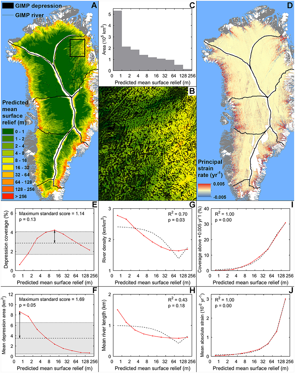
Figure 11. (A) Predicted mean surface relief map compared with the distribution of GIMP-DEM derived closed surface depressions of the whole ice sheet (B) and GIMP-DEM derived rivers of NE Greenland. (C) Area covered by the predicted mean surface relief categories of the GrIS is also shown; categories smaller than 4,500 km² have been removed. (D) The ice sheet wide principal strain rate is shown as well. (E) The coverage (F) and mean area of the GIMP-DEM derived depressions corresponding to predicted mean surface relief categories has been calculated from the ice sheet wide depression dataset. (G) The density (H) and mean length of the GIMP-DEM derived rivers, (I) the mean absolute principal strain rate (J) and the coverage of the area where principal strain rates exceed +0.005 yr⁻¹ are also provided in the same manner for the whole ice sheet. Maximum standard scores, with their corresponding p-values, and the best-fit quadratic trends (dashed line), with their corresponding R² and p-values, are shown where applicable.

Estimating the Pattern of Surface Drainage on Future and Palaeo Ice Sheets

Previous studies have predicted the evolution of surface drainage on the GrIS during the twenty-first century, by using runoff and surface mass balance projections, and contemporary surface DEMs of the ice sheet (Leeson et al., 2015; Ignéczi et al., 2016). These studies have considered the potential influence of basal topography, but assumed fixed ice sheet geometry and focussed their projections solely on temporal variations in the distribution of surface lakes caused by changes in surface mass balance. Since temporally-evolving ice thickness will affect the spatial distribution of surface undulations, the validity of these projections are limited to relatively short durations: perhaps several decades or a century. On longer time scales, changing ice thickness will modify the topographic transfer and the pattern of mesoscale surface relief which strongly preconditions the drainage pattern (Figure 12). Although higher-order ice sheet models are capable of simulating the necessary topographical details, the computational costs of producing such simulations at the required spatial resolution limit their applicability for ice sheet-scale problems. A way of circumventing this problem is to use the non-stationary integral method in Equations (1) and (2), explored in this paper, whereby the mesoscale surface relief is calculated from bed topography DEMs, available at relatively high resolution, and modeled surface topography and flow state, which are available at lower resolution (Ng et al., 2018). This approach extends the timescale of projection of surface drainage on ice sheets. However, as the transfer equations assume a steady state, the response time of the surface topography to the changing conditions, that control the transfer of basal variability to the surface (e.g., ice thickness, basal slip ratio), may somewhat limit the precision of such projections (Ng et al., 2018).

FIGURE 12

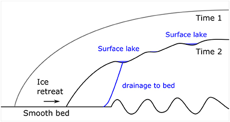
Figure 12. Concept of how an evolution of ice sheet geometry over time modifies the transfer of basal variability to the surface, and thus the spatial structure of surface drainage.

Our approach can also be applied to reconstruct the mesoscale surface relief of palaeo ice sheets using available bed topography DEMs and ice sheet model outputs. Hitherto, subglacial pathways of the Antarctic and Greenland Ice Sheets have been reconstructed for the last deglaciation cycle (Livingstone et al., 2013), but not their supraglacial drainage. As the potential surface meltwater inputs (location and magnitude) into the reconstructed subglacial drainage systems are unknown, inferences of the ice sheet response, i.e., advance/retreat rates, to changes in hydrology are limited. As we have demonstrated, mesoscale surface relief can be considered a proxy for surface drainage, so our method opens up the possibility to reconstruct the large-scale pattern of surface drainage on palaeo ice sheets. This could aid the empirical evaluation of the long-term response (>10² years) of ice sheets to changes in the surface and subglacial drainage.

Conclusions

We have demonstrated that it is possible to predict the large-scale pattern of surface relief on the GrIS from ice sheet-wide bed topography, ice thickness and basal slip ratio datasets, by using a non-stationary integral method (Ng et al., 2018) employing Gudmundsson's (2003) linearized transfer functions. The mismatch found between the observed and predicted surface relief—or “relief anomaly”—arises from unknown basal slipperiness variations, uncertainties of the bed topography and basal slip ratio datasets, surface processes on the ice sheet, the assumption of a linearly viscous medium, and 3D effects on the transfer of basal variability. The spatial pattern of the relief anomaly is consistent with the expected consequences caused by the assumption of linearly viscous ice and the 2D approximations of the transfer of basal variability. Our results also suggest that surface processes and the seasonal variability of ice flow exhibit only a secondary influence on mesoscale surface topographical undulations.

Our analyses show that basal topography preconditions the large-scale structure of the surface drainage system on the GrIS, while other factors such as surface runoff generation and crevassing influence the temporal evolution of drainage (i.e., when, where, and to what degree drainage develops compared to the maximum potential) within a particular melt season. Surface depressions and lakes have the largest coverage in areas with moderate surface relief, while the spatial density of surface rivers decrease and the density of moulins increase with increasing surface relief. In conclusion, we suggest that the greatest potential for surface meltwater injections into the subglacial drainage system occurs where the bed-to-surface topography transfer and thus the surface relief are moderately high, due to the presence of both a high density surface drainage system and moulins/crevasses.

A key source of uncertainty in the prediction of surface relief of the GrIS is inconsistent quality of the bed DEM. Indeed, the quality of bed DEMs for contemporary ice sheets is poor compared to other terrestrial environments. Despite this, our approach yields a good match between the observed and predicted surface relief of the contemporary GrIS. Good quality DEMs have been made available recently for the beds of paleo-ice sheets (e.g., ArcticDEM) and the precision and spatiotemporal resolution of ice sheet reconstructions are quickly improving (e.g., Clark et al., 2012; Hughes et al., 2016). Hence, our new approach has a strong potential to ascertain the spatio-temporal evolution of surface drainage during major deglaciations. Comparing this with the pattern of ice sheet retreat could provide the first quantification of the long-term (>10² years) effects of hydrology on ice sheet mass balance and dynamics.

Author Contributions

ÁI, AS, and SL designed the project. ÁI wrote the manuscript. FN developed the transfer equations as published in Ng et al. (2018); these were coded and implemented by ÁI and FN. AS calculated the principal strain rates and SL mapped the moulins from the SETSM-DEM. KY provided his previously published Landsat-8 derived lake, river, and moulin dataset. The data was integrated and analyzed by ÁI. All authors discussed the results and commented on the manuscript.

Conflict of Interest Statement

The authors declare that the research was conducted in the absence of any commercial or financial relationships that could be construed as a potential conflict of interest.

The reviewer HP and handling editor declared their shared affiliation.

Acknowledgements

ÁI acknowledges the support of a Ph.D. grant from the Ice and Climate Research at Sheffield (ICERS), University of Sheffield and ÁI, SL, and AS acknowledge the support of the White Rose University Consortium Collaboration Fund grant awarded to AS and SL. FN is supported by a UK Leverhulme Trust Research Fellowship (no. RF-2017-320). KY is supported by the National Natural Science Foundation of China (41501452) and the Fundamental Research Funds for the Central Universities. We thank the National Snow & Ice Data Center (NSIDC) for making available the MEaSUREs GIMP surface DEM from GeoEye and WorldView Imagery (Version 1), IceBridge BedMachine Greenland (Version 3) and the MEaSUREs Greenland Ice Sheet Velocity Map from InSAR data (Version 2). We also acknowledge the U.S. Geological Survey's Earth Resources Observation and Science (EROS) for making Landsat-8 data available. We are sincerely grateful for the support of Myoung-Jong Noh and Ian Howat, who provided the SETSM DEM, Xavier Fettweis who provided the MAR runoff outputs, and Joseph MacGregor who provided the basal slip ratio estimations. This work benefitted from discussions with Chris Clark and David Rippin. We also thank the three reviewers for their constructive criticism.

Supplementary Material

The Supplementary Material for this article can be found online at: https://www.frontiersin.org/articles/10.3389/feart.2018.00101/full#supplementary-material

References

Alessio, S. (2016). Digital Signal Processing and Spectral Analysis for Scientists. Cham: Springer.

Google Scholar

Banwell, A., Arnold, N., Willis, I., Tedesco, M., and Ahlstrøm, A. (2012). Modeling supraglacial water routing and lake filling on the Greenland Ice Sheet. J. Geophys. Res.117:F04012. doi: 10.1029/2012JF002393

CrossRef Full Text | Google Scholar

Bartholomew, I., Nienow, P., Mair, D., Hubbard, A., King, M., and Sole, A. (2010). Seasonal evolution of subglacial drainage and acceleration in a Greenland outlet glacier. Nat. Geosci. 3, 408–411. doi: 10.1038/ngeo863

CrossRef Full Text | Google Scholar

Black, H., and Budd, W. (1964). Accumulation in the region of Wilkes, Wilkes Land, Antarctica. J. Glaciol. 5, 3–15. doi: 10.1017/S0022143000028549

CrossRef Full Text | Google Scholar

Catania, G., and Neumann, T. (2010). Persistent englacial drainage features in the Greenland Ice Sheet. Geophys. Res. Lett. 37:L02501. doi: 10.1029/2009GL041108

CrossRef Full Text | Google Scholar

Christoffersen, P., Bougamont, M., Hubbard, A., Doyle, S. H., Grigsby, S., and Petterson, R. (2018). Cascading lake drainage on the Greenland Ice Sheet triggered by tensile shock and fracture. Nat. Commun. 9, 1064. doi: 10.1038/s41467-018-03420-8

PubMed Abstract | CrossRef Full Text | Google Scholar

Clark, C., Hughes, A., Greenwood, S., Jordan, C., and Sejrup, H. (2012). Pattern and timing of retreat of the last British-Irish Ice Sheet. Quat. Sci. Rev. 44, 112–146. doi: 10.1016/j.quascirev.2010.07.019

CrossRef Full Text | Google Scholar

Das, S. B., Joughin, I., Benn, M., Howat, I., King, M., Lizarralde, D., et al. (2008). Fracture propagation to the base of the Greenland Ice Sheet during supraglacial lake drainage. Science 320, 963–964. doi: 10.1126/science.1153360

PubMed Abstract | CrossRef Full Text | Google Scholar

De Rydt, J., Gudmundsson, H., Corr, J., and Christoffersen, O. (2013). Surface undulations of Antarctic ice streams tightly controlled by bedrock topography. Cryosphere 7, 407–417. doi: 10.5194/tc-7-407-2013

CrossRef Full Text | Google Scholar

Echelmeyer, K., Clarke, T., and Harrison, W. (1991). Surficial glaciology of Jakobshavn Isbrae, West Greenland: part I. Surface-morphology. J. Glaciol. 37, 368–382. doi: 10.1017/S0022143000005803

CrossRef Full Text | Google Scholar

Enderlin, E., Howat, I., Jeong, S., Noh, M., Angelen, J., and van den Broeke, M. (2014). An improved mass budget for the Greenland ice sheet. Geophys. Res. Lett. 41, 866–872. doi: 10.1002/2013GL059010

CrossRef Full Text | Google Scholar

Fettweis, X., Box, J., Agosta, C., Amory, C., Kittel, C., Lang, C., et al. (2017). Reconstructions of the 1900-2015 Greenland ice sheet surface mass balance using the regional climate MAR model. Cryopshere 11, 1015–1033. doi: 10.5194/tc-11-1015-2017

CrossRef Full Text | Google Scholar

Flowers, G. (2015). Modelling water flow under glaciers and ice sheets. Proc. R. Soc. A 471:20140907. doi: 10.1098/rspa.2014.0907

PubMed Abstract | CrossRef Full Text | Google Scholar

Gow, J., and Rowland, R. (1965). On the relationship of snow accumulation to surface topography at “Byrd Station”, Antarctica. J. Glaciol. 5, 843–847.

Google Scholar

Gudmundsson, H. (2003). Transmission of basal variability to a glacier surface. J. Geophys. Res. 108:2253. doi: 10.1029/2002JB002107

CrossRef Full Text | Google Scholar

Gudmundsson, H., Raymond, C., and Bindschadler, R. (1998). The origin and longevity of flow stripes on Antarctic ice streams. Ann. Glaciol. 27, 145–152. doi: 10.3189/1998AoG27-1-145-152

CrossRef Full Text | Google Scholar

Hoffman, M. J., Perego, M., Andrews, L. C., Price, S. F., Neumann, T. A., Johnson, J. V., et al. (2018). Widespread moulin formation during supraglacial lake drainages in Greenland. Geophys. Res. Lett. 45, 778–788. doi: 10.1002/2017GL075659

CrossRef Full Text | Google Scholar

Howat, I., Negrete, A., and Smith, B. (2014). The Greenland Ice Mapping Project (GIMP) land classification and surface elevation data sets. Cryosphere 8, 1509–1518. doi: 10.5194/tc-8-1509-2014

CrossRef Full Text | Google Scholar

Howat, I., Negrete, A., and Smith, B. (2017). Measures Greenland Ice Mapping Project (GIMP) Digital Elevation Model from GeoEye and WorldView Imagery, Version 1. Boulder, CO: NASA National Snow and Ice Data Center Distributed Active Archive Center.

Hughes, A., Gyllencreutz, R., Lohne, Ø., Mangerud, J., and Svendsen, J. (2016). The last Eurasian ice sheets – a chronological database and time-slice reconstruction, DATED-1. Boreas 41, 1–45. doi: 10.1111/bor.12142

CrossRef Full Text

Ignéczi, Á., Sole, A., Livingstone, S., Fettweis, X., Selmes, N., Gourmelen, N., et al. (2016). Northeast sector of the Greenland Ice Sheet to undergo the greatest inland expansion of supraglacial lakes during the 21st century. Geophys. Res. Lett. 43, 9729–9738. doi: 10.1002/2016GL070338

CrossRef Full Text | Google Scholar

IPCC (2013). “Climate change 2013: the physical science basis” in Contribution of Working Group I to the Fifth Assessment Report of the Intergovernmental Panel on Climate Change, eds T. F.Stocker, D. Qin, G. K. Plattner, M. Tignor, S. K. Allen, J. Boschung, A. Nauels, Y. Xia, V. Bex, and P. M. Midgley (Cambridge UK; New York, NY: Cambridge University Press), 1535.

Irvine-Fynn, T., Hodson, A., Moorman, B., Vatne, G., and Hubbard, A. (2011). Polythermal glacier hydrology: a review. Rev. Geophys. 49:RG4002. doi: 10.1029/2010RG000350

CrossRef Full Text | Google Scholar

Joughin, I., Das, S., Flowers, G., Behn, M., Alley, R., King, M., et al. (2013). Influence of ice-sheet geometry and supraglacial lakes on seasonal ice-flow variability. Cryosphere 7, 1185–1192. doi: 10.5194/tc-7-1185-2013

CrossRef Full Text | Google Scholar

Joughin, I., Smith, B., Howat, I., and Scambos, T. (2017). MEaSUREs Greenland Ice Sheet Velocity Map from InSAR Data, Version 2. Boulder, CO: NASA National Snow and Ice Data Center Distributed Active Archive Center.

Joughin, I., Smith, B., Howat, I., Scambos, T., and Moon, T. (2010). Greenland flow variability from ice-sheet-wide velocity mapping. J. Glaciol. 56, 415–430. doi: 10.3189/002214310792447734

CrossRef Full Text | Google Scholar

Karlstrom, L., and Yang, K. (2016). Fluvial supraglacial landscape evolution on the Greenland Ice Sheet. Geophys. Res. Lett. 43, 2683–2692. doi: 10.1002/2016GL067697

CrossRef Full Text | Google Scholar

Kingslake, J., Ng, F., and Sole, A. (2015). Modelling channelized surface drainage of supraglacial lakes. J. Glaciol. 61, 185–199. doi: 10.3189/2015JoG14J158

CrossRef Full Text | Google Scholar

Krawczynski, M., Behn, M., Das, S., and Joughin, I. (2009). Constrains on the lake volume required for hydrofracture through ice sheets. Geophys. Res. Lett. 36:L10501. doi: 10.1029/2008GL036765

CrossRef Full Text | Google Scholar

Lampkin, D., and Vanderberg, J. (2011). A preliminary investigation of the influence of basal and surface topography on supraglacial lake distribution near Jakobshavn Isbrae, western Greenland. Hydrol. Process. 25, 3347–3355. doi: 10.1002/hyp.8170

CrossRef Full Text | Google Scholar

Leeson, A., Shepherd, A., Briggs, K., Howat, I., Fettweis, X., Morlighem, M., et al. (2015). Supraglacial lakes on the Greenland Ice Sheet advance inland under warming climate. Nat. Clim. Change 5, 51–55. doi: 10.1038/nclimate2463

CrossRef Full Text | Google Scholar

Leeson, A., Shepherd, A., Palmer, S., Sundal, A., and Fettweis, X. (2012). Simulating the growth of supraglacial lakes at the western margin of the Greenland Ice Sheet. Cryosphere 6, 1077–1086. doi: 10.5194/tc-6-1077-2012

CrossRef Full Text | Google Scholar

Livingstone, S., Clark, C., Woodward, J., and Kingslake, J. (2013). Potential subglacial lake locations and meltwater drainage pathways beneath the Antarctic and Greenland ice sheets. Cryosphere 7, 1721–1740. doi: 10.5194/tc-7-1721-2013

CrossRef Full Text | Google Scholar

Lüthje, M., Pedersen, L. T., Reeh, N., and Greuell, W. (2006). Modelling the evolution of supraglacial lakes on the west Greenland Ice Sheet margin. J. Glaciol. 52, 608–618. doi: 10.3189/172756506781828386

CrossRef Full Text | Google Scholar

MacGregor, J. A., Fahnestock, M., Catania, G., Aschwanden, A., Clow, G., Colgan, W., et al. (2016). A synthesis of the basal thermal state of the Greenland Ice Sheet. J. Geophys. Res. Earth Surf. 121, 1328–1350. doi: 10.1002/2015JF003803

PubMed Abstract | CrossRef Full Text | Google Scholar

Mallat, S. (2009). A Wavelet Tour of Signal Processing: The Sparse Way, 3rd Edn. Burlington: Academic Press.

Medley, B., Ligtenberg, S., Joughin, I., van den Broeke, M., Gogineni, S., and Nowicki, S. (2015). Antarctic firn compaction rates from repeat-track airborne radar data: I. Methods Ann. Glaciol. 44, 263–272. doi: 10.3189/2015AoG70A203

CrossRef Full Text | Google Scholar

Morlighem, M., Rignot, E., Mouginot, J., Seroussi, H., and Larour, E. (2014). Deeply incised submarine glacial valleys beneath the Greenland ice sheet. Nat. Geosci. 7, 418–422. doi: 10.1038/ngeo2167

CrossRef Full Text

Morlighem, M., Williams, C., Rignot, E., An, L., Arndt, J., and Bamber, J. (2017a). IceBridge BedMachine Greenland, Version 3. Boulder, CO: NASA National Snow and Ice Data Center Distributed Active Archive Center.

Morlighem, M., Williams, C., Rignot, E., An, L., Arndt, J., Bamber, J., et al. (2017b). BedMachine v3: complete bed topography and ocean bathymetry mapping of Greenland from multi-beam echo sounding combined with mass conservation. Geophys. Res. Lett. 44, 11051–11061. doi: 10.1002/2017GL074954

CrossRef Full Text | Google Scholar

Ng, F. S. L., Ignéczi, A., Sole, A. J., and Livingstone, S. J (2018). Response of surface topography to basal variability along glacial flowlines. J. Geophys. Res. Earth Surf. doi: 10.1029/2017JF004555

CrossRef Full Text | Google Scholar

Noh, M.-J., and Howat, I. (2015). Automated stereo-photogrammetric DEM generation at high latitudes: surface extraction with TIN-based search-space minimization (SETSM) validation and demonstration over glaciated region. GISci. Remote Sens. 52, 198–217. doi: 10.1080/15481603.2015.1008621

CrossRef Full Text | Google Scholar

Poinar, K., Joughin, I., Das, S., Behn, M., Lenaerts, J., and van den Broeke, M. (2015). Limits to future expansion of surface-melt-enhanced ice flow into the interior of western Greenland. Geophys. Res. Lett. 42, 1800–1807. doi: 10.1002/2015GL063192

CrossRef Full Text | Google Scholar

Poinar, K., Joughin, I., Lilien, D., Brucker, L., Kehrl, L., and Nowicki, S. (2017). Drainage of southeast Greenland firn aquifer water through crevasses to the bed. Front. Earth Sci. 5:5. doi: 10.3389/feart.2017.00005

CrossRef Full Text | Google Scholar

Price, S. F., Hoffman, M., Bonin, J., Howat, I., Neumann, T., Saba, J., et al. (2017). An ice sheet model validation framework for the Greenland ice sheet. Geosci. Model Dev. 10, 255–270. doi: 10.5194/gmd-10-255-2017

PubMed Abstract | CrossRef Full Text | Google Scholar

Raymond, J., and Gudmundsson, H. (2005). On the relationship between surface and basal properties on glaciers, ice sheets, and ice streams. J. Geophys. Res. 110:B08411. doi: 10.1029/2005JB003681

CrossRef Full Text | Google Scholar

Rippin, D. (2013). Bed roughness beneath the Greenland ice sheet. J. Glaciol. 59, 724–732. doi: 10.3189/2013JoG12J212

CrossRef Full Text | Google Scholar

Ross, N., Sole, A., Livingstone, S., Ignéczi, Á., and Morlighem, M. (2018). Near-margin ice thickness from a portable radar: implications for subglacial water routing, Leverett Glacier, Greenland. Arct. Antarct. Alp. Res. 50:e1420949. doi: 10.1080/15230430.2017.1420949

CrossRef Full Text | Google Scholar

Selmes, N., Murray, T., and James, T. (2011). Fast-draining lakes on the Greenland Ice Sheet. Geophys. Res. Lett. 38:L15501. doi: 10.1029/2011GL047872

CrossRef Full Text | Google Scholar

Sergienko, O. (2013). Glaciological twins: basally controlled subglacial and supraglacial lakes. J. Glaciol. 59, 3–8. doi: 10.3189/2013JoG12J040

CrossRef Full Text | Google Scholar

Shepherd, A., Hubbard, A., Nienow, P., King, M., McMillan, M., and Joughin, I. (2009). Greenland ice sheet motion coupled with daily melting in late summer. Geophys. Res. Lett. 36:L01501. doi: 10.1029/2008GL035758

CrossRef Full Text | Google Scholar

Smith, L., Chu, V., Yang, K., Gleason, C., Pitcher, L., Rennermalm, A., et al. (2015). Efficient meltwater drainage through supraglacial stream and rivers on the southwest Greenland ice sheet. Proc. Natl. Acad. Sci. U.S.A. 112, 1001–1006. doi: 10.1073/pnas.1413024112

CrossRef Full Text | Google Scholar

Sole, A., Mair, D., Nienow, P., Bartholomew, I., King, M., and Burke, M. (2011). Seasonal speedup of a Greenland marine terminating outlet glacier forced by surface melt-induced changes in subglacial hydrology. J. Geophys. Res. 116:F03014. doi: 10.1029/2010JF001948

CrossRef Full Text | Google Scholar

Sole, A., Nienow, P., Bartholomew, I., Mair, D., Cowton, T., Tedstone, A., et al. (2013). Winter motion mediates dynamic response of the Greenland Ice Sheet to warmer summers. Geophys. Res. Lett. 40, 3940–3944. doi: 10.1002/grl.50764

CrossRef Full Text | Google Scholar

Stevens, L. A., Behn, M., McGuire, J., Das, S., Joughin, I., Herring, T., et al. (2015). Greenland supraglacial lake drainages triggered by hydrologically induced basal slip. Nature 522, 73–76. doi: 10.1038/nature14480

PubMed Abstract | CrossRef Full Text | Google Scholar

Sundal, A., Shepherd, A., Nienow, P., Hanna, E., Palmer, S., and Huybrechts, P. (2009). Evolution of supra-glacial lakes across the Greenland Ice Sheet. Remote Sens. Environ. 113, 2164–2171. doi: 10.1016/j.rse.2009.05.018

CrossRef Full Text | Google Scholar

Tedstone, A. J., Nienow, P., Gourmelen, N., Dehecq, A., Goldberg, D., and Hanna, E. (2015). Decadal slowdown of a land-terminating sector of the Greenland Ice Sheet despite warming. Nature 526, 692–695. doi: 10.1038/nature15722

PubMed Abstract | CrossRef Full Text | Google Scholar

van As, D., Hubbard, A., Hasholt, B., Mikkelsen, A., van den Broeke, M., and Fausto, R. (2012). Large surface meltwater discharge from the Kangerlussuaq sector of the Greenland ice sheet during the record-warm year 2010 explained by detailed energy balance observations. Cryosphere 6, 199–209. doi: 10.5194/tc-6-199-2012

CrossRef Full Text | Google Scholar

van den Broeke, M., Bamber, J., Ettema, J., Rignot, E., Schrama, E., van de Berg, W., et al. (2009). Partitioning recent Greenland mass loss. Science 326, 984–986. doi: 10.1126/science.1178176

PubMed Abstract | CrossRef Full Text | Google Scholar

van de Wal, W., Boot, W., van den Broeke, M., Smeets, C., Reijmer, C., Donker, J., et al. (2008). Large and rapid melt-induced velocity change in the ablation zone of the Greenland Ice Sheet. Science 321, 111–114. doi: 10.1126/science.1158540

CrossRef Full Text | Google Scholar

Whillans, I. (1975). Effect of inversion winds on topographic detail and mass balance on inland ice sheets. J. Glaciol. 14, 85–90. doi: 10.1017/S0022143000013423

CrossRef Full Text | Google Scholar

Yang, K., and Smith, L. (2016). Internally drained catchments dominate supraglacial hydrology of the southwest Greenland Ice Sheet. J. Geophys. Res. Earth Surf. 121, 1891–1910. doi: 10.1002/2016JF003927

CrossRef Full Text | Google Scholar

Zwally, H. J., Abdalati, W., Herring, T., Larson, K., Saba, J., and Steffen, K. (2002). Surface melt-induced acceleration of Greenland Ice-Sheet flow. Science 297, 218–222. doi: 10.1126/science.1072708

PubMed Abstract | CrossRef Full Text | Google Scholar