Snow Cover Change as a Climate Indicator in Brunswick Peninsula, Patagonia

Introduction and Regional Setting

Climate change particularly affects snow-covered areas (Hughes, 2003; IPCC, 2013), since even small changes in the surface–atmospheric energy balance may cause significant decreases in snow cover, affecting the local hydrology, associated ecosystems, hydroelectric power generation, and tourism activities (Gobiet et al., 2014; McGowan et al., 2018). Therefore, if climate trends can be detected, valuable information can be provided to decision makers and stakeholeders.

Snow cover is a critical component of the cryosphere and climate system at both local and global scales (Chen et al., 2018). Snow also affects other components of the Earth system at different scales by its radiative and thermal properties which modulate transfer of energy and mass at the surface-atmosphere interface (Frei et al., 2012). Snow cover can affect glaciers through changes in albedo and mass balance and also affects permafrost through its thermal insulation properties and meltwater input (Beniston et al., 2018). Additionally, snow is critical for water resources during the melt season, especially in areas lacking glaciers. Snow occurrence is also relevant for regional planning, including vehicle traffic, pasture and livestock management, its retarding effect on flash floods and slope erosion during extreme precipitation events and winter tourism and sports. In fact, snow-based tourism and sport was identified as particularly vulnerable to climate change. This climate dependency together with its economic impact on ski tourism (Steiger and Abegg, 2018), has prompted the authorities and private sector of the Magallanes Region in austral Chile to re-think the future of the current ski resort “Club Andino” located at Cerro Mirador, close to Punta Arenas city, which has barely operated for 10 days in the last two snow seasons (2016–2017). A possible alternative is a new ski resort planned to be located at Tres Morros, 25 km southwest and 200 m higher than Cerro Mirador.

The climate along the west coast of southern South America, including southern Patagonia, is determined by the permanent high pressure anticyclonic circulation (the subtropical South Pacific High, SPH) located in the south-eastern Pacific Ocean centered around 30°S, the circumpolar low pressure belt that surrounds the Antarctic continent around 60°S, and the resulting westerly wind regime that prevails in mid-latitudes (40–55°S). The seasonal north-south displacement of the SPH and the circumpolar trough modulate the westerly flow, and therefore, defines the eastward trajectory of the low-pressure frontal systems that cross southern South America. In particular, the west side of southernmost Patagonia is frequently affected by passing fronts and low-pressure systems that results in a high number of cloudy (77–86%) and precipitation days (81–88%) throughout the year (Carrasco et al., 2002). In addition, the complex topography defines a distinct climate regime at both sides of the Andes, with a relatively warmer and moister environment on the western side in comparison with the eastern side (Schneider et al., 2003; Weidemann et al., 2018). The precipitation is much higher and increases with altitude on the western slope due to orographically induced upward motion, and rapidly decreases toward the east due to the foehn mechanism (Weidemann et al., 2013).

The scarcity of rain-gauge stations precludes exhaustive regional and temporal analysis. The last IPCC report (Hartmann et al., 2013) reveals this difficulty. Their assessment indicates a negative trend of the annual precipitation ranging between 5 and 10 (2.5 – 5) mm per decade around Punta Arenas for the 1901–2010 (1951–2010) period using the GHCN (Global Historical Climatology Network of NOAA) dataset on the western coast of Patagonia (see their Figure 2.29). Earlier, Carrasco et al. (2008), analyzing the 1958–2006 period, showed an overall increase of the precipitation registered at the Punta Arenas airport from around 1967 to 1991, but no trend thereafter. Later, González-Reyes et al. (2017) with data updated to 2014, indicated that large interannual and inter-decadal precipitation variability has been observed for the last 100 years at Punta Arenas. Although a long-term trend is not evident from this record, a significant precipitation reduction has been observed after 1990, especially in spring and summer, while the winter precipitation has shown a significant increase.

Furthermore, an overall temperature increase has been detected in southern South America. Early work by Ibarzábal et al. (1996) and Rosenblüth et al. (1997) suggested that the warming has been higher in the eastern side of the Andes than on its western side. Falvey and Garreaud (2009) showed a strong temperature contrast in central and northern Chile (17° – 37°S) for the 1979-2006 period, with a coastal cooling of −0.2°C/decade and warming of +0.25°C/decade only 100–200 kilometers further inland. This cooling could be linked to an intensification of the South Pacific Anticyclone during recent decades, that enhances ocean upwelling off the coast of Chile. However, a recent study suggests that this recent period of coastal cooling has ended, modulated by a phase change of the Interdecadal Pacific Oscillation (Burger et al., 2018).

Therefore, there is a need for systematic studies to characterize the spatial and temporal distribution of snow cover in the Southern Hemisphere, and particularly in southernmost Patagonia, since all of the scarce long-term in-situ records from South America are from the central Andes (Vaughan et al., 2013). Here, we reduce this gap by using a remote sensing approach based on MODIS satellite data to reconstruct a snow cover time series and to relate snow conditions to present and past climate variations. This study is framed within a broader science programme that aims at contributing snow and climate information for regional planning in the Magallanes Region in southernmost Chile. The main problem we wish to target is whether snow cover has shown significant changes during the last few decades at Brunswick Peninsula, and if so, which are the main forcing factors. As such, this article will contribute to predict the future snow evolution in the area of Punta Arenas, the largest Chilean city in southern Patagonia.

Study Area

The study area is located on Brunswick Peninsula in southern Patagonia between 52.9° and 53.9°S and 73.0° and 70.4°W. This peninsula is part of the southern extension of the Patagonian Andes where Punta Arenas is the largest city and capital of the Magallanes Region, the southernmost region of Chile. It is surrounded by the Strait of Magellan to the east, and by Seno Otway to the west. Most of the southwestern part is dominated by small mountains of the southern Andes, with many summits between 500 and 1,000 m, but all lower than 1,200 m a.s.l. Contrastingly, the northeastern part exhibits mostly a flat topography below 200 m a.s.l., which is part of the Patagonian steppe (“pampa”). The first mountains to the south are located west of Punta Arenas, with a maximum altitude of 590 m a.s.l. at Cerro Mirador. On the eastern slope of this summit the skiing resort “Club Andino” is located at 53.15°S, 71.05°W. A future skiing resort is planned at “Tres Morros” at 53.31°S, 71.29°W, 866 m a.s.l., located 25 km SW of Cerro Mirador. The area has a strong Pacific Ocean influence, through the prevailing westerly circulation regime. This in combination with the unique topographic distribution of the Patagonian Andes creates one of the most pronounced precipitation gradients on earth (Carrasco et al., 2002; Schneider et al., 2003; Smith and Evans, 2007; Garreaud et al., 2013; Weidemann et al., 2018). Due to the north-south orientation of the Andes almost perpendicular to the westerly airflow, the regional west-to-east variation along the 53°S latitude and across the southern Andes shows an annual precipitation of about 6,000 mm on the western slopes of the mountain range decreasing to < 1,000 mm on the eastern slope (Schneider et al., 2003) and to 416 mm at Punta Arenas (González-Reyes et al., 2017).

Figure 1 shows the geographical location and the three different specific study areas where the snow-cover variability has been reconstructed. The first chosen area is the “Macro zone” of 1,637 km² covering a large part of the Brunswick Peninsula, used here as representative of the snow cover distribution on the entire peninsula. Two smaller embeded zones are respectively centered on the existing ski resort “Cerro Mirador” (302 km²) and the projected ski resort “Tres Morros” (291 km²). These two locations, during the time frame of the analysis, proved to have less cloud coverage than the southern Macro zone area, allowing adequate snow sensing by visible and near-infrared MODIS imagery.

FIGURE 1

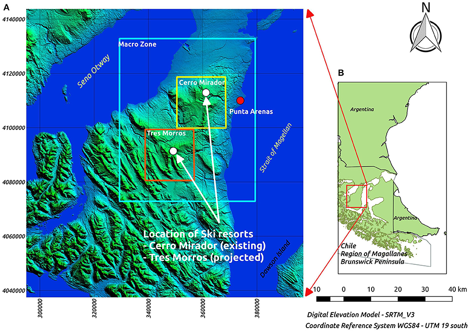
Figure 1. General view of the study area. (A) shows the Brunswick Peninsula with the three study zones: Macro zone of 1637 km² (cyan), Cerro Mirador of 302 km² (yellow), and Tres Morros of 291 km² (red). The terrain elevation is shown with a DEM from SRTM_V3 data. (B) presents the general location of the study area.

Data and Method

In this section we describe the different data and methods used to reconstruct the inter-annual snow cover variability and the spatial and temporal evolution. Data include MODIS satellite information, ground stations, radiosonde, and MERRA-2 reanalysis. Calculations including snow reconstruction and statistical applications were made using the open source programing language Python v._3.5 (http://www.python.org). Maps (Figures 1, 2) were depicted using the open source QGIS v_2.18¹ A couple of figures (9 and 13B) were made using Matplotlib Python graphic package (Hunter, 2007).

FIGURE 2

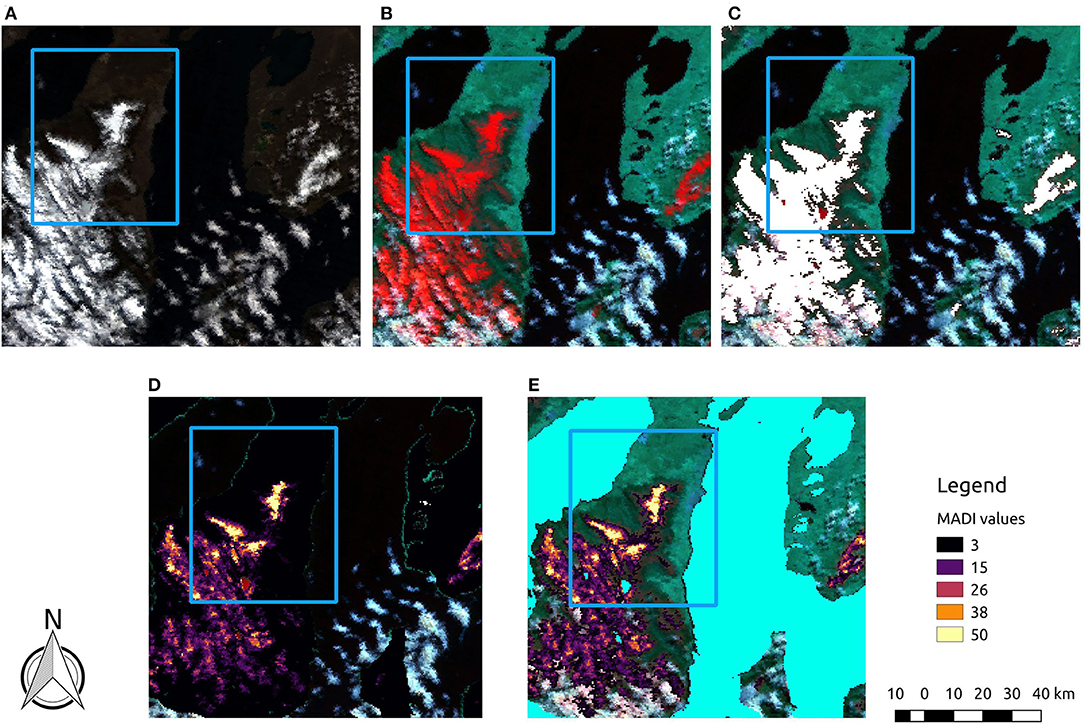
Figure 2. MODIS-derived snow cover for the 26th of August 2015. (A) True color composition (1-4-3 MODIS bands), snow and clouds are both represented in white color. (B) False-color composite (MODIS bands 3-6-7) with snow in red and clouds in white. (C) NDSI mask, snow in white color. (D) MADI index, purple to light yellow colors show smaller to larger values, and clouds in white color. (E) Overlay of MADI values over the false color composite on snow covered areas as inferred from the NDSI mask, and the water mask in cyan. The macro zone limits are shown as a blue rectangle.

MODIS Data and Snow Cover Detection

To reconstruct the extent of the seasonal snow cover at Brunswick Peninsula, we take advantage of the snow spectral reflectance properties given by the Moderate Resolution Imaging Spectroradiometer (MODIS) satellite data at 500 meters spatial resolution. The high temporal resolution (< 2 days) of MODIS data facilitates selection of cloud-free imagery at the latitude of Brunswick Peninsula. Additionally, its multispectral capabilities make it one of the most advanced optical sensors available for large-scale terrestrial applications (Salomonson et al., 1989).

Several MODIS products are available, including the MOD10 snow cover data in its version MOD10A1 (daily) and MOD10A2 (8-day composite). Both products use the Normalized Difference Snow Index (NDSI) algorithm based on MODIS reflectance data of bands 4 and 6 to discriminate snow from other targets (Winther and Hall, 1999; Sirguey et al., 2009). This method is usually preferred instead of other classification methods such as the supervised classification (Wang and Li, 2003).

The MODIS cloud product (MOD35) is also incorporated into the algorithm to construct the snow products. Nevertheless, inaccurate detection of clouds show some problems in high elevation regions such as the Southern Alps of New Zealand (Hall et al., 2002; Sirguey et al., 2009) and the Northern Patagonia Icefield (Lopez et al., 2008; Sirguey et al., 2009). Some corrections have been implemented in updated versions of the snow cover product but snow and cloud discrimination problems persist (Hall and Riggs, 2007). Recurrent misclassifications limit the suitability of the MOD10 snow product for detecting the snow cover in frequently cloud-covered regions, such as southernmost Patagonia.

Therefore in this study we use the MODIS land product MOD09GA from the Terra satellite in its version 6 (Vermote and Wolfe, 2015) at daily temporal resolution. We did not include the MODIS land product derived from the Aqua satellite due to malfunctioning of one of the spectral bands (Saavedra et al., 2018). The product MOD09GA includes corrected reflectance with a spatial resolution of 500 m (available from the Land Processes Distributed Active Archive Center, http://lpdaac.usgs.gov/) for the period 2000–2016. To optimize the download process, we used the script “order_MWS.pl” (available from https://ladsweb.modaps.eosdis.nasa.gov/tools-and-services/), downloading a total of 6079 images. We downloaded the satellite data covering approximately an area of 31,500 km², in order to obtain a general view and select image subsets.

To better discriminate potential cloud cover we conducted a visual inspection of the all images, which resulted in a selection of 484 could-free images. Sixty percent of the selected images (290) correspond to the period between April to September, temporal frame that we name “extended winter”. At least, there is one cloud-free image for each extended winter month between 2000 and 2016, except for May and August 2000. Figure 2 shows an example as a comparison between true-color (RGB: spectral MODIS bands B1, B4, B3) and false-color (RGB: spectral MODIS bands B3, B6, B7) compositions to help selecting cloud-free imagery.

A water mask was generated using the coastal margin of the Regional Government of Magallanes (http://www.goremagallanes.cl) and the information of lakes from the Dirección General de Aguas, (DGA, General Water Management of Chile, http://www.dga.cl/productosyservicios/mapas/Paginas/default.aspx#nueve) to exclude any possible interference between the snow detection and water bodies during in the analysis.

Snow Detection Indices

There are several alternative methods for snow detection using different sensors and wavelengths. In this work, we computed two different indices from MOD09GA bands 1, 4, 6 and 7 (specified below): the NDSI and the Melt Area Detection Index (MADI). Both indices plus the calculation of the new proposed Index (Snow_power index), were applied to each selected image and subsequently grouped to monthly means to obtain a monthly representation of the snow cover.

Normalized Difference Snow Index

NDSI is the most common method used for detection of the snow cover (Frei and Lee, 2010). It uses the contrast between the high reflectance (ρ) of snow in the green part of the visible spectrum (MODIS band 4, 545–565 nm) and the low reflectance in the short-wave infrared part of the spectrum (MODIS band 6, 1,628–16,52 nm). We used the threshold value NDSI ≥ 0.4 (Hall et al., 2002) for identification of snow pixels based on:

$\begin{array}{ll}NDSI=\frac{{\rho }_{B4}-{\rho }_{B6}}{{\rho }_{B4}+{\rho }_{B6}}.& (1)\end{array}$

Melt Area Detection Index

The MADI approach uses the reflectance ratio between the red portion of the visible spectrum (MODIS spectral band 1, 0.62–0.67 μm) and the near-infrared (MODIS spectral band 7, 2.105–2.155 μm). Its principle is based on identifying liquid water layers that coat snow and ice when melt occurs to discriminate between frozen and liquid water (Chylek et al., 2007) according to:

$\begin{array}{ll}MADI=\frac{{\rho }_{B1}}{{\rho }_{B7}}& (2)\end{array}$

MADI has been usually used to detect wet and dry snow over regions of known snow cover only. A study carried out by Bormann et al. (2012) in Australia considered a suitable threshold for snow cover detection similar to the NDSI method. This method establishes ranges for the MADI values using in-situ observations for snow detection. If the MADI value exceeds 6, then the pixel is characterized as snow. Additionally, Bormann et al. (2012) used the MADI values to infer snow depth validated with in-situ observations.

We combine the MADI and NDSI according to the following two steps procedure (see Figure 2):

1. We detect snow cover area (km²) inside of each study zone. For this purpose, the NDSI is used as a binary snow cover detector representing snow-cover extent.

2. For the area detected above, we apply the MADI to each pixel classified as snow. Using a zonal mean we obtain a zonal representation expressed as a weight indicator of snow depth, according to Bormann et al. (2012).

With these two different indices we reconstruct and compare the inter-annual variability of snow cover for the period 2000–2016. Therefore, the NDSI is used to detect snow pixels and MADI is incorporated in a newly proposed index, called Snow_power, that incorporates the performance of both indices. We used the following equation for computing Snow_power index:

$\begin{array}{ll}SNO{W}_{power}(i)=\frac{\overline{{\displaystyle \sum NDS{I}_{mask}}}(i)\times {\overline{MADI}}_{zonalaverage}(i)}{\max (\overline{{\displaystyle \sum NDS{I}_{mask}}})}& (3)\end{array}$

Where $\overline{{\displaystyle \sum NDS{I}_{mask}}(i)}$ is the monthly average of the snow cover extension (pixels) for month (i), ${\overline{MADI}}_{zonalaverage}(i)$ is the zonal average MADI value for all snow-covered areas for the month (i), and $\max \left(\overline{{\displaystyle \sum NDS{I}_{mask}}}\right)$ is the maximum snow cover monthly NDSI value for all months considered.

Thus, this index is the result of the percentage of snow cover presence (NDSI) in a given area scaled by the zonal average MADI values for all the snow cover extent, divided by the present snow cover and its maximum monthly value for all months considered. We postulate that this relationship represents better the snow cover since it incorporates both snow cover fraction, in each zone of interest, and a weight linking it to snow depth obtained by MADI so that we derive the variability of the entire snowpack. In this study, we use both the snow cover extent using only NDSI, and the Snow_power index as a combination of NDSI and MADI indices.

Meteorological Data and Climate Indices

Weather Station Data

A major difficulty in Patagonia is the scarcity of locally observed meteorological data, since weather stations are restricted to the main settlements and many stations have significant data gaps. A main weather station is Carlos Ibáñez Airport (53.00°S, 70.53°W, 38 m a.s.l), 18 km to the north of Punta Arenas city center. It has permanent atmospheric observations since 1958 and belongs to the Dirección Meteorológica de Chile (DMC, the National Chilean Weather Service). In 1970 the Instituto de la Patagonia deployed the weather station “Jorge Schythe” (Santana et al., 2009) at 53.07°S and 70.52°W at 5 m a.s.l, within the city of Punta Arenas, 14 km south of the Punta Arenas Airport. In 1973 DGA (Dirección General de Aguas) installed at Jorge Schythe station a pluviometer, a thermometer and a relative humidity sensor. Data are available for Jorge Schythe station at a monthly level since 1972, and at a daily level since 1980. Another long-term meteorological record (more than 100 years) is also available from the Navy station Evangelistas Lighthouse (52.24°S, 75.06°W, 55 m a.s.l.) located at the western entrance of the Strait of Magellan.

The available station data allow studying the inter-annual and decadal pattern of air temperature and precipitation in relation to forcing mechanisms such as the El Niño Southern Oscillation (ENSO), the Antarctic Oscillation (AAO) or the Southern Annular Mode (SAM), and the Pacific Decadal Oscillation (PDO). Other stations have been deployed in recent decades in southern South America by DGA (e.g., Teniente Merino, San Gregorio, Pampa Huanaco and Bahía San Felipe), by DMC (Porvenir station) and by specific research projects such as Bahamondes station (Schneider et al., 2003; Weidemann et al., 2018). Table 1 lists the above stations used in this study.

TABLE 1

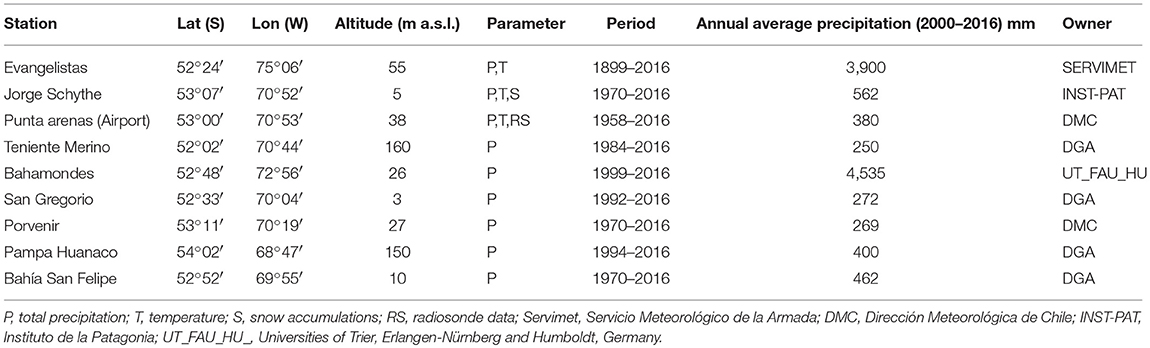
Table 1. Weather stations used in this research.

Radiosonde Data Punta Arenas

At Punta Arenas airport, radiosonde balloons are launched every day at 12 UTC (Universal Time Coordinated) since April 1975. This upper-air station measures a daily vertical profile of air temperature, relative humidity, wind direction and wind speed at different standard levels of the atmosphere. The zero-isotherm altitude (ZIA) can be determined from the air temperature profile. Monthly radiosonde data can be obtained from the Anuario Climatológico (Climatological Yearbook) available online from www.meteochile.gob.cl. Here, monthly averages of surface air temperature and 850 hPa (hectopascal) levels were used to determine the monthly altitudinal lapse rate which along with the geopotential height at the 850 hPa allowed to calculate the monthly and annual ZIA.

Reanalysis Data

The monthly snow cover product from MERRA-2 reanalysis data (“fractional snow-covered area FRSNO”) for April–September (Gelaro et al., 2017) period were used for comparison with the MODIS snow cover reconstruction from 1980 to 2016. MERRA-2 data were downloaded from https://giovanni.gsfc.nasa.gov. MERRA-2 has a resolution of 0.5° × 0.625° latitude-longitud grid with 72 model layers interpolated to 42 standard pressure levels (Bosilovich et al., 2015). It uses the modified three-layer snow model of Lynch-Stieglitz (1994). This snow hydrology model resolves for snow melting and refreezing, as well as dynamic changes in snow density, snow insulating properties, and other physics relevant to the growth and ablation of the snowpack (Stieglitz et al., 2001). The snow model component of the Land Surface Model (LSM) uses the minimum snow water equivalent (WEMIN) before it considers the surface to be snow covered (Reichle, 2012). In this sense, if the amount of snow (SNOMAS) on a given model-surface area is insufficient to cover the entire area with at least an amount of WEMIN, the snow cover fraction (FRSNO) will be the fraction of the area that is covered by an amount equal to WEMIN, that is expressed as, FRSNO = min(1, SNOMAS/WEMIN) (Reichle, 2012; Reichle et al., 2017). No studies have so far been conducted on how well the MERRA-2 can simulate snow cover in Patagonia.

The MERRA-2 snow cover values were extracted for the grid point 53.3°S, 71.1°W within the Macro zone. The values are expressed as a monthly snow cover fraction, with a value of 1 representing 100% of snow cover. For example, the maximum monthly FRSNO value for the period 2000–2016 was 0.38 for June 2002, when the NDSI snow cover extent indicated an area of 1,443 km² for the Macro zone, equivalent to 88% of the total domain area of 1,637 km².

Climate Indices

ENSO is the most significant mode of inter-annual climate variability in the Southern Hemisphere with world-wide impacts. El Niño (La Niña) corresponds to the warm (cold) phase which is characterized by weaker (stronger) trade winds and above (below) normal sea surface temperatures (SST) in the equatorial Pacific Ocean. Also, a weaker (stronger) SPH is encountered during El Niño (La Niña) with stronger (weaker) subtropical and weaker (stronger) polar jet-streams (Chen et al., 1996). In southernmost South America, a weak correlation between ENSO and precipitation occurs to the west of the Patagonian Andes between 45° and 55°S (Schneider and Gies, 2004), i.e., with below (above) normal precipitation during El Niño (La Niña) (Montecinos and Aceituno, 2003).

The PDO, also called Interdecadal Pacific Oscillation (IPO) has a cycle of 15–30 years that shows similar SST and sea-level pressure anomaly patterns as ENSO (Garreaud and Battisti, 1999; Mantua and Hare, 2002). During the warm (or positive) PDO phase, El Niño events prevail in frequency and intensity. On the contrary, during the cool (or negative) phase, the opposite pattern occurs and La Niña episodes are more frequent and last longer (Andreoli and Kayano, 2005). In southern Patagonia the prevailing large-scale pattern associated with a positive PDO is an anticyclonic circulation centered in the southeastern Pacific Ocean to the west of the Antarctic Peninsula (Garreaud and Battisti, 1999). This pattern might reduce precipitation along the southern tip of South America, so that the storm systems may be steered northwards (Garreaud and Battisti, 1999).

Another natural internal mechanism for interannual variability is related to the SAM (also known as the Antarctic Annular Oscillation AAO) a large-scale alternation of atmospheric pressure between the mid-latitudes and high latitudes at the surface pressure level (Gong and Wang, 1999). These changes are linked with changes in the strength of the Southern Hemisphere westerly winds due to the latitudinal shift in the area of maximum zonal flow (~45°S) or in its intensity (surface wind speed) (Moreno et al., 2010). Positive correlations between the westerlies and precipitation prevail along the western margin of the southern South America between 40° and 55°S, while correlations tend to be negative at similar latitudes along the Atlantic margin (Moreno et al., 2010). Thus positive (negative) AAO means southward (northward) displacement of the westerlies, and therefore, of the storm track in the Pacific Ocean. This can also favor (inhibit) precipitation events in the western coast of southern South America, although it depends how far the southward (northward) displacement extends and whether the area of interest is governed by orographic rain or rather by foehn effects on the east side of the Cordillera.

These different mechanisms are expressed by their respective indices. The interannual variability of ENSO can be studied by using SOI, a normalized sea-level pressure difference between Tahiti and Darwin stations (Chen, 1982; Trenberth, 1997). Alternatively, among other indices, the SST monthly anomalies in the central-equatorial sector of the Pacific Ocean, known as Niño 3.4 can be employed as an ENSO index (Trenberth, 1997). The PDO index is calculated by the leading principal component applied to the spatial monthly averaged SST of the North Pacific Ocean north of 20°N, using mainly the October to March period so that the interannual fluctuation mostly takes place in winter (Mantua and Hare, 2002). The AAO is calculated by principal component analysis so that the first three modes explain 33, 11 and 9% of the variance, respectively, and it can be constructed using the 700 hPa height anomalies poleward of 20°S (Gong and Wang, 1999). The above indices were downloaded from the Earth System Research Laboratory www.esrl.noaa.gov/psd/data/climateindices/list/, specifically, the SOI from www.cpc.ncep.noaa.gov/data/indices/soi, the PDO from www.esrl.noaa.gov/psd/ data/correlation/pdo.data and the AAO from www.esrl.noaa.gov/psd/data/correlation/aao.data.

Statistical Analysis

In order to analyse the variability of snow cover extent, statistical correlations were performed with different climate variables. We use the Pearson correlation quantified by the coefficient of determination (R²), the Durbin-Watson statistics for detecting autocorrelation between variables, and significance tests with t-statistic using a p-value at 5% significance. The structure of the residuals is also analyzed to detect any biases. Based on the best relationship we express the satellite-derived snow cover as a function of climate variables, which allows to reconstruct the snow cover to 1965. In order to detect long-term trends we use an exponential filter (Rosenblüth et al., 1997) to reduce the interannual variability and apply a linear regression. Python Statsmodels statistic package was used (Seabold and Perktold, 2010).

Results

Climate Variability and Trends

Precipitation and Temperature From Surface Stations

The average monthly precipitation 2000–2016 for 8 weather stations aligned from west to east around 53°S is shown in Figure 3. Precipitation is much higher (around one order of magnitude) in the western stations Evangelistas and Bahamondes located in the windward side of the Andes than the stations located in the leeward side (for example Punta Arenas). Precipitation occurs year-round with only little seasonality, although the minimum (maximum) tends to occur at the end of winter (summer)—beginning of spring (autumn). In general, precipitation increases from north to south although Bahía San Felipe station shows higher accumulation than Pampa Huanaco located further south. The annual variability during the 2000–2016 period is displayed in Figure 4. There are no correlations among different stations except between the two nearby ones located in Punta Arenas (airport and city). This reveals the large spatial variability of precipitation in southernmost South America. Also, no common and significant trends can be observed in the analyzed stations. Thus, while Evangelistas suggests an increase, Punta Arenas city and Bahía San Felipe suggest instead a decrease in precipitation in the last 17 years. This finding was already mentioned by González-Reyes et al. (2017) who analyzed the long-term behavior for the 1900-2014 period using precipitation data from Observatorio Meteorológico Monseñor Fagnano located in Punta Arenas city center (where the Salesian mission began measurements in 1887) and Punta Arenas Airport where observations started in 1930. The Airport station was first located in Bahía Catalina until 1958, 4 km north of the city center, and then moved 14 km north to Punta Arenas Airport (Presidente Carlos Ibáñez del Campo) where DMC continues the measurements at present. González-Reyes et al. (2017) found a significant reduction in the annual precipitation sums after 1990, especially in spring and summer, while the winter precipitation showed a significant increase during that period.

FIGURE 3

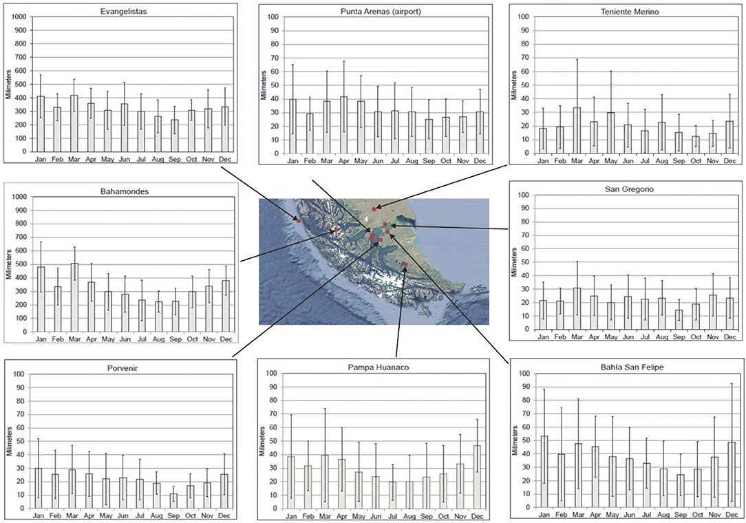
Figure 3. Monthly precipitation averages over the period 2000–2016. Vertical lines are the 1st standard deviation. The red dot immediately south of Punta Arenas corresponds to Jorge Schythe station at Instituto de la Patagonia located in Punta Arenas city, shown in Figure 4. Note that the vertical scale at Evangelistas and Bahamondes stations (the two western locations) have a range of 1,000 mm, while the range for all the other stations is 100 mm.

FIGURE 4

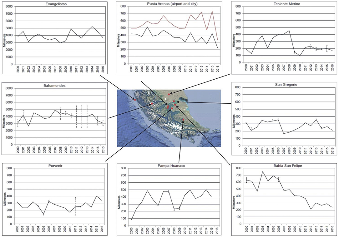
Figure 4. Annual precipitation time series for the 2000–2016 period. Vertical lines in some graphs are the sum of the 1st standard deviation of the missing months, which were replaced by their respective monthly averages. Note that the vertical range at Evangelistas and Bahamondes stations (the two western locations) is 8,000 mm, while all other stations have a range of 800 mm.

The other long-term precipitation record is from Evangelistas with data available from 1899 onward, operated by the Chilean Navy. Monthly data and some complete years are missing which preclude exhaustive analysis. Nevertheless, 80% of the data are available and only 8 years have more than 6 months missing, with 3 complete years missing. Figure 5 shows the annual and extended winter (April–September) annual variability and longterm trend of precipitation. It was constructed using the Evangelistas data, the missing monthly averages were replaced by the respective long-term monthly averages to facilitate data management. The vertical lines on the annual data are the sum of the 1st standard deviation of the missing months which assigns an upper and lower boundary for the most probable annual precipitation. The solid curve results by applying an exponential filter to the data to eliminate the inter-annual variability and highlighting the interdecadal variability (Essenwanger, 1986; Rosenblüth et al., 1997). This filter is similar to a moving mean, but it has the advantage of keeping the complete series for analyzing relatively short periods.

FIGURE 5

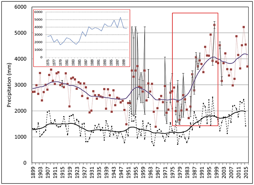
Figure 5. Annual precipitation (red squares) at Evangelistas station over the period 1989–2016. The purple curve is the result of an exponential filter applied to smooth the original annual data (squares). Vertical lines in some years are the sum of the 1st standard deviation of the missing months, which were replaced by their respective monthly averages. The upper left inset shows a zoom of the 1975–2000 period. Lower curves (black) are the extended-winter (April-September) precipitation at Evangelistas station.

The annual data show an overall decrease in precipitation from 1899 until 1980, after which a significant increase took place between 1984 and 1998. The precipitation decline observed by González-Reyes et al. (2017) during 1990–2014 at Punta Arenas is not completely captured by the Evangelistas data, although an overall decrease could have taken place during 1997–2007. The significant precipitation increase from around 1984–1998 has been a matter of discussion of whether it is a real signal or rather a result of an instrument change or relocation of instrument or change in staff and operation mode (Carrasco et al., 2002; Aravena and Luckman, 2009). According to the Servicio Meteorológico de la Armada (Navy Weather Service) the weather station has not been changed in location, nor the instrument type or operation mode, only the staff is replaced every one or 2 years (personal communication Ismael Escobar, Chilean Navy). The insert in Figure 5 shows an enlargement of the 1975–2000 period, suggesting a rapid but gradual increase of precipitation. However, the magnitude of the increment (of about 70% between 1984 and 1998) should be taken with caution, even though Evangelistas is located just to the south of the maximum precipitation region (Miller, 1976) and a slight southward displacement of the westerlies could indeed trigger such profound change in overall precipitation.

Figure 6A shows the monthly average of the mean air temperature at Evangelistas, Bahamondes and Punta Arenas Airport over the 2000–2016 period. The ocean and continental influences are clearly seen by comparing the annual cycle at each station located in the latitudinal transect around 53°S. The average winter (summer) air temperature at Punta Arenas Airport is about 3 (2)°C colder (warmer) than at Evangelistas. The inter-annual variability and the long-term trend (solid lines) of the extended winter (April–September) mean temperatures for Evangelistas and Punta Arenas are shown in Figure 6B for the available 1965–2016 and 1958–2016 periods, respectively. The temperature trends within both periods show a significant warming in all seasons (especially in the winter) including the montly mean and minimum temperatures. A total warming of 0.54°C (0.11°C/decade) and 0.72°C (0.12°C/decade) is found at Evangelistas and Punta Arenas Airport over the 1965–2016 and 1958–2016 periods, respectively, computed using the interannual extended winter data (smoothed data).

FIGURE 6

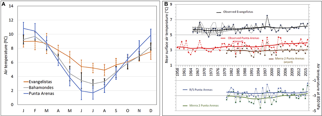
Figure 6. (A) Annual cycle of mean air temperature at Punta Arenas Airport, Evangelistas and Bahamondes stations for the 2000–2016 period. Vertical lines are the 1st standard deviation. (B) Extended winter (April–September) mean air temperatures (dashed lines) at Evangelistas (upper curve, black) and Punta Arenas airport (lower curve, red) over the period 1958–2016. Thick lines are the result of an exponential filter applied to smooth the annual data (squares). Dashed (solid) gray curves in the annual (filtered) Evangelistas data are the lower and upper boundary of the sum of the 1st standard deviation of the missing months which were replaced by their respective monthly averages. Brown solid and dashed lines are the near surface air temperature as simulated by the MERRA-2 model at the nearest gridpoint from Punta Areans. (C) Winter mean air temperature at 850 hPa measured by the radiosonde (R/S) at Punta Arenas (blue lines) and simulated by the MERRA-2 model for the nearest gridpoint from Punta Arenas (green lines). Solid lines are the smooth behavior after applying the exponential filter, while dashed lines are the interannual variability. MERRA-2 data are available from 1980 onward.

Upper Air Sounding

The analysis of upper air data from Punta Arenas Airport is restricted for the lower half troposphere given by the standard levels at 850, 700, and 500 hPa which respectively correspond to the annual (January-December) mean altitudes of 1,338, 2,856, and 5,377 m. This corresponds to an annual mean air temperature of −1.5, −9.7, and −26.1°C, respectively. The chosen levels show positive linear trends of +0.01, +0.25, and +0.45°C (non-statistically significant) over the 1976–2016 period at 850, 700, and 500 hPa, respectively, revealing a moderate warming trend in the mid-troposphere. Also, the zonal component of the wind (u-wind) at surface, 850, 700, and 500 hPa shows positive linear trends of 0.81, 1.73, 2.39, and 2.45 ms⁻¹ for the 1976–2016 period, respectively (Figure 7). The increase in wind speeds is not statistically significant. However, this finding might be indicative of southernmost South America becoming more and more affected by a windier environment due possibly to the enhancement and southward displacement of the westerly winds associated with positive SAM during recent decades (Marshall, 2003). Following the analysis of Schneider and Gies (2004) and Garreaud et al. (2013), the correlation between precipitation and u-wind at 850 hPa reveals that with stronger zonal wind there is an increase in precipitation westward from the Patagonian Andes and a decrease over the eastern side. The overall different behavior of the precipitation observed at Evangelistas and Punta Arenas may be the result of the overall increase in the u-wind component.

FIGURE 7

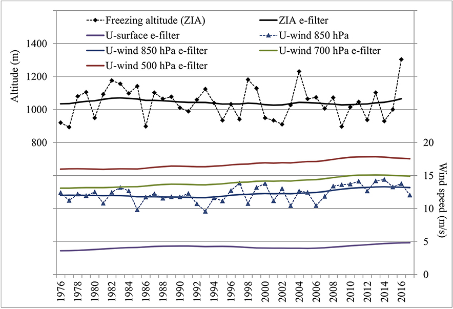
Figure 7. Annual and long-term (using an exponential filter) Zero Isotherm Altitude (ZIA) (black) and zonal wind component at surface (purple), 850 hPa (blue), 700 hPa (green) and 500 hPa (red) from Punta Arenas Airport radiosonde data.

The mean annual freezing level calculated from the radiosonde data shows a 49 m non-statistically significant increase during the 1976–2016 period. The highest freezing level recorded in the period occurred in 2016 with an altitude of 1,304 m, 263 m higher than the average in the whole period (see Figure 7). The year 2016 also showed the lowest annual precipitation since 1970 according to the Punta Arenas Airport station record.

Snow Cover Reconstruction and Variability

In Figure 8, we show the monthly average of the snow cover area using the NDSI and the MADI indices for each domain namely the Macro zone, Cerro Mirador, and Tres Morros (Figure 1). We assume that the beginning and the end of the snow season occur when the monthly snow cover extent rises or drops below 20% of the multi-year maximum montly snow extent, that is 327 km² for the Macro zone, 58 km² for Cerro Mirador and 60 km² for Tres Morros.

FIGURE 8

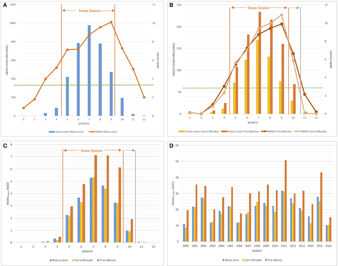
Figure 8. Monthly average representation of the snow cover area and the Snow_power index for 2000–2016. (A) shows the mean monthly snow cover area, the MADI index and the duration of the snow season in the Macro zone. (B) Represents the same snow properties for the sub-regions Cerro Mirador and Tres Morros. (C) Provides monthly averages of the Snow_power index for the period 2000–2016, and (D) shows the monthly Snow_power index sums for 2000–2016 for each zone. The green line on (A,B) represents 20% of the multi-year maximum monthly snow extent on each zone, which is used for inferring the beginning and the end of the snow season. The gray line on (B,C) represents the extent of the snow season on Tres Morros in comparison to Cerro Mirador.

With this approach, we can identify the annual duration of the snow season which usually begins in May and ends in September for Cerro Mirador and in October for Tres Morros. The relation between the snow cover area and MADI values is shown in Figure 8. The monthly averaged snow cover duration is 4 weeks longer at Tres Morros compared to Cerro Mirador due to higher altitudes. Similar Snow_power index values can be observed between Macro and Cerro Mirador zones, while Tres Morros shows higher values due to its higher altitude.

Figure 9 shows scatter plots between the Snow_power index and the snow cover extent derived from the NDSI and MADI indices. Coefficient of determination (R²-values) higher than 0.86 are obtained for the Snow_power index between each pair of zones especially between the Macro zone and Cerro Mirador (R² = 0.96, Figure 9A). This is reasonable considering that the Macro zone includes the other two zones and considers a more varied topography. A slightly smaller Snow_power index R² = 0.86 is obtained between Cerro Mirador and Tres Morros (Figure 9C), which can be attributed to its higher altitude which results in a larger and more permanent snow cover extent, unlike to the case of Cerro Mirador.

FIGURE 9

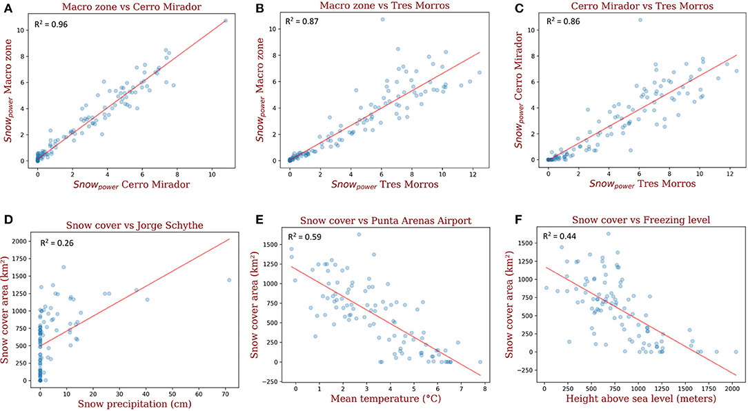
Figure 9. Scatter plots. (A–C) show the correlation of the Snow_power index between each study zones and the coefficient of determination (R²). (D–F) show the correlations of the MODIS reconstructed snow cover on the Macro zone between the most relevant climatic variables at a monthly level during the extended winter: snow precipitation at Jorge Schythe station, mean temperatute at Punta Arenas Airport, and freezing level at Punta Arenas Airport.

At Cerro Mirador the ski club “Club Andino” has recorded information of the ski season duration based on the opening and closing dates of the ski lifts and the snow height average during the ski season from a stake located close to the main hut. There is no artificial snow production at the ski club so the start and end of the ski season depends largely on snow precipitation and air temperature, with a minimum natural snow height requirement of about 20 cm without compaction to start the skiing operation. Since 2010 the longest season occurred in 2015 with 95 snow-days (representing the duration of the skiing season) and an average snow height of 140 cm. Figure 10A displays the relation between the duration of the ski season for the Macro zone and Cerro Mirador and its reconstructed snow cover extent from the NDSI index. We use the June-August period for the ski season, when most of the skiing activity is concentrated. The linear correlation between the ski season duration (days) and the Cerro Mirador snow cover (Figure 10B) is R² = 0.94, and R² = 0.87 for Macro Zone (Figure 10C). The correlation of the ski season duration with the Snow_power index is also good but somewhat smaller, with R² = 0.77 for Cerro Mirador and R² = 0.83 for the Macro Zone, respectively. The correlation between of the average snow height from Club Andino with the NDSI snow cover extent (Snow_power index) is not as good as the correlation with the ski season duration, with R² = 0.72 (0.80) and R² = 0.75 (0.67) for the Macro Zone and Cerro Mirador, respectively. Based on these results, hereafter we consider the NDSI snow cover extent as a better indicator of snow cover variability than the Snow_power index.

FIGURE 10

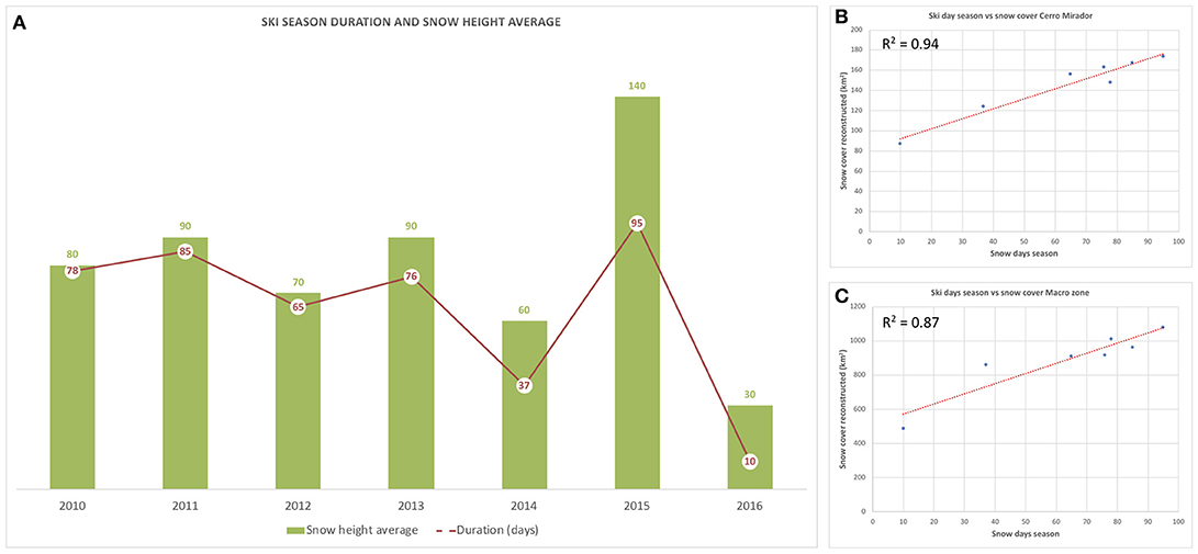
Figure 10. Ski season duration and snow height average. (A) shows the relationship between the ski season duration and the average snow height measured at Club Andino. (B,C) display the correlation between the duration of the ski season and the monthly averaged NDSI-reconstructed snow cover from June-August (average of of the ski season period), for the Cerro Mirador and Macro zone, respectively. Both correlations are significant at the 95% confidence level.

Figure 11 shows the climate indices and snow cover of the Macro zone at Brunswick Peninsula after smoothing the interannual variability using the exponential filter (Rosenblüth et al., 1997) over the 2000–2016 period. It reveals the overall positive trend of the AAO, i.e., the southward displacement of the westerly winds, which could be linked with the decrease of the snow cover shown within the Macro zone. On the other hand, the PDO almost concurs with the decadal behavior of the snow cover. Thus, it seems that periods with positive (negative) PDO result in lower (higher) snow cover in the Brunswick Peninsula. Individual year-to-year variability given by El Niño and La Niña phases does not show a direct relation with snow cover behavior, although strong El Niño (La Niña) events tend to concur with less (more) snow cover and precipitation in the study area. This could be due to the interannual AAO that can also suppress or favor precipitation in the southern tip of South America.

FIGURE 11

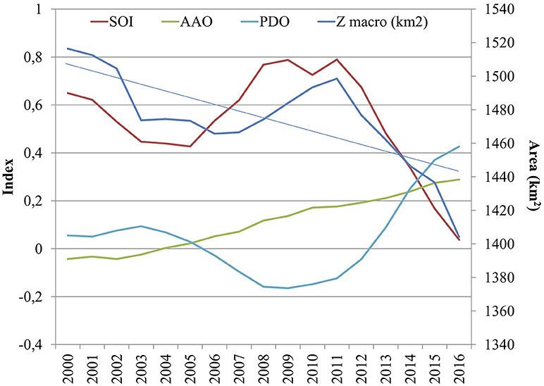
Figure 11. Climate indices and snow cover at Brunswick Peninsula after smoothing the interannual variability using an exponential filter. The straight light blue line is the linear trend of the snow cover. SOI: Southern Oscillation Index (red), AAO: Antarctic Oscillation Index (green), PDO: Pacific Decadal Oscillation Index (black). Z macro (blue) is the snow cover extent (km2) on the study area (Brunswick Peninsula).

Figure 12 shows the number of precipitation days with air temperature < 2°C during April and September (extended winter) for each year for the 1958–2016 period at Punta Arenas Airport, along with the average of air temperature for these days. Also displayed is the air temperature average during days following a snow event. Results indicate a warming of 0.65°C (p < 0.05) for precipitation days over the 1958–2016 period. On average, 11.3 ± 4.4 (±1 standard deviation) of precipitation days with air temperature < 2°C occur during the extended winter in the period 1958–2016. These days are regarded as “snow days”, revealing a decline of 11% (1.2 “snow days,” p < 0.05) over the 1958–2016 period. The long-term behavior obtained after applying the exponential filter to the interannual variability shows an increase from 1958 to 1971 and from 1982 to 1999, as well as a decrease from 1972 to 1981 and also from 2000 to 2016. During 2000-2016 the linear trend indicates a decrease of 18% (2 “snow days,” p < 0.05). The mean air temperature for days following the snow events reveals a slight positive trend of 0.27°C (p < 0.05) over the 1958–2016 period, of 0.52°C (p < 0.05) over the 1973–2016 period and of 0.55°C (p < 0.05) over the 2000–2016 period. In summary, this analysis indicates an overall decrease of snow precipitation days along with an overall increase of the air temperature, mostly concentrated in recent decades (Figure 12).

FIGURE 12

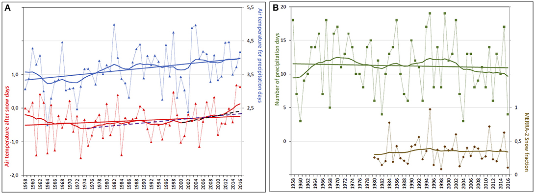
Figure 12. Interannual variability, long-term behavior (after applying the exponential filter) and linear trend of: (A) mean air temperature for precipitation days (rain and snow) (blue, upper section) and for days after snow events (red, lower section). The dashed purple and black lines (lower section) are the linear trends for the 1973–2016 and 2000–2016 periods, respectively. (B) Number of precipitation days with air temperature < 2°C for each year (green, upper section). The brown curve (lower section) is the snow fraction obtained from the MERRA-2 simulation. All variables are expressed as annual data calculated for the extended winter April to September.

Figure 12 includes as well the snow fraction obtained from the MERRA-2 reanalysis data. Correlations of R² = 0.16 (p < 0.05) are obtained between the snow fraction and air temperature after snow events; R² = 0.41 (p < 0.05) between the snow fraction and air temperature during precipitation days; and R² = 0.42 (p < 0.05) between snow fraction and air temperature during “snow days.”

Discussion

The snow cover reconstruction can be analyzed in relation to climate variables at a montly and annual level, such as freezing level (upper air sounding at Punta Arenas Airport), snow accumulation (measured daily at Jorge Schythe and modeled at Punta Arenas Airport), and minimum and average temperatures (at Jorge Schythe and Punta Arenas Airport). These variables were chosen because of the better correlation with the snow cover (summary shown in Table 2). The measured daily snow accumulation data are limited to the Jorge Schythe station only, published here for the first time. We use a threshold relation with air temperature to derive the solid/liquid precipitation fraction to infer snow accumulation [c(i)] at Punta Arenas Airport, as indicated by Schaefer et al. (2013), as follows:

$\begin{array}{ll}c\left(i\right)=q\left(i\right)\times P(i)& (4)\end{array}$

Where q(i) is the solid part of the total precipitation, prescribed by temperature as:

$\begin{array}{ll}q(i)=\{\begin{array}{c}ifT\left(i\right)>Utthenq(I)=0\\ ifLt\le T\left(i\right)\le Utthenq\left(i\right)=\frac{Ut-T(i)}{1^{\underset{\_}{°}}C}\\ ifT\left(i\right)<Ltthenq(i)=1\end{array}& (5)\end{array}$

Where T(i) is the mean air temperature (°C), calculated as the average between the daily maximum and minimum air temperatures, P(i) is the daily total (liquid and solid) precipitation accumulation (mm), Ut and Lt are upper and lower temperature thresholds (°C).

TABLE 2

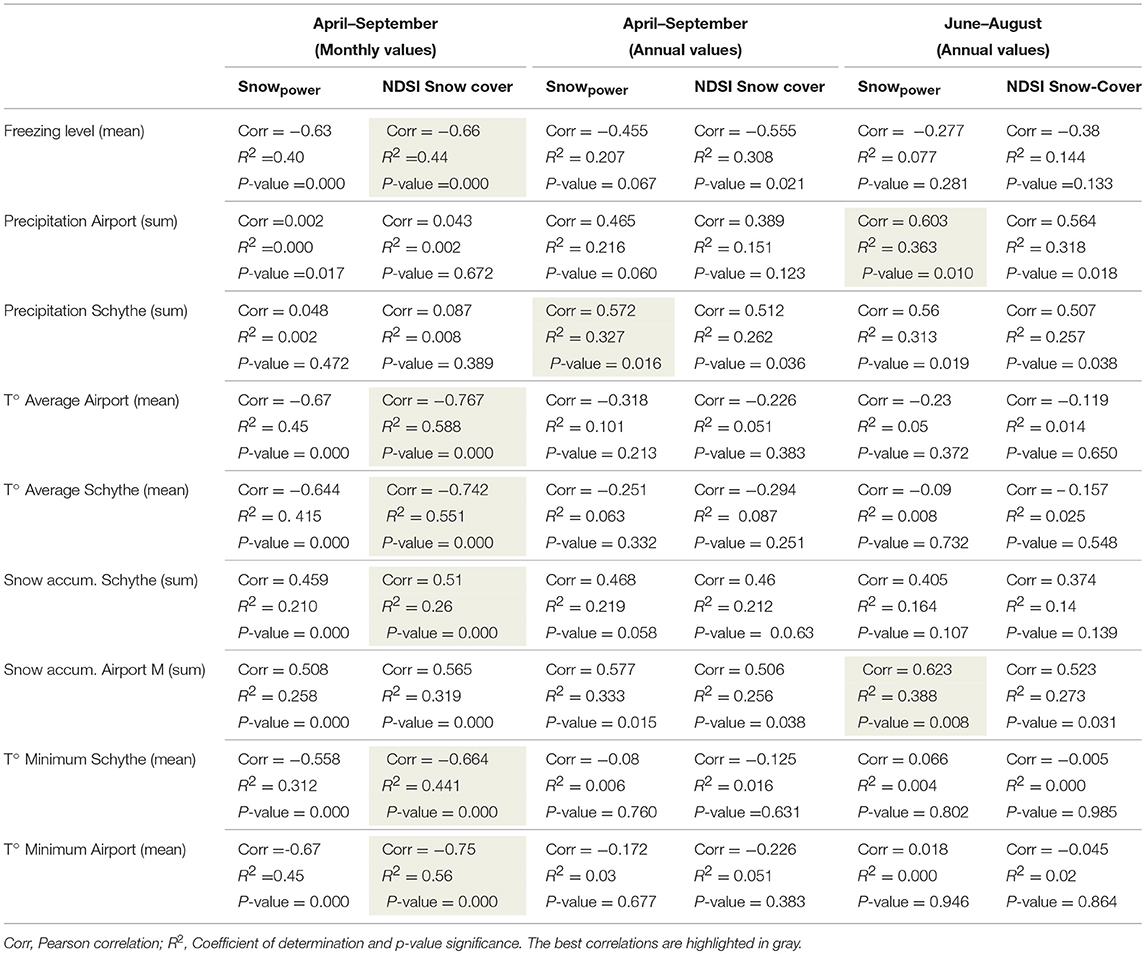
Table 2. Result of the different linear regressions between Snow_power index and NDSI snow cover (km²) for the Macro zone, with the Punta Arenas Airport freezing level from radiosonde data, precipitation (mm), minimum, and mean temperature (monthly averages) from Punta Arenas Aiport and Jorge Schythe stations, for two different periods in 2000–2016: April–September (monthly and annual values) and June–August (annual).

Ut and Lt were estimated as 1.6 and 0.9°C, respectively. These values were determined through a sensitivity analysis using the daily snow accumulation and mean air temperature at Jorge Schythe for 1980–2016. In our case Ut and Lt are slightly larger than the values of 1.5 and 0.5°C assumed by Schaefer et al. (2013) for the Northern Patagonia Icefield. The modeled precipitated snow has a correlation of R² = 0.48 with the measured snow values at a daily level, R² = 0.76 for monthly values, and R² = 0.88 for annual values. Equation (5), based on daily values, was applied at Punta Arenas Airport to infer its monthly snow accumulation.

In this analysis we only used the Macro zone indices due to the high level of correlation with the other two study zones (Figure 9). This allows to extend back the period of analysis earlier than the year 2000 in order to identify long-term trends of snow cover behavior. Based on these results, to find a better relationship for explaining snow cover variability, we tested both simple and multiple linear regressions.

The multiple regressions with the best significant correlation for the MODIS snow cover reconstructed for the Macro zone in the period 2000–2016 was found using the monthly snow accumulation and the mean monthly temperature, with R² = 0.62 (Equation 6, which allows to model the snow cover for the period 1972–2016), and R² = 0.62 (Equation 7, which allows to model the snow cover for 1958–2016 period), both statistically significant at 95% (Figure 13). Temperatures were chosen at the Airport station to avoid possible urban effects at Jorge Schythe station located within the city of Punta Arenas. Correlations for the “extended winter” period from April to September were better than the annual (January–December) and the winter (June–July–August) correlations.

FIGURE 13

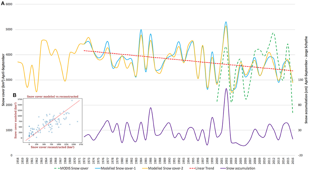
Figure 13. (A) Upper section. Annual (April–September sums) of NDSI snow cover reconstructed for the Macro zone from MODIS data (dashed green) for the period 2000–2016. The annual (April–September sums) of snow cover modeled with Equation (6) (snow cover as a function of monthly mean temperature at Punta Arenas Airport and snow accumulation at Schythe station) is shown in light blue for the 1972–2016 period, while the red dashed line represents its linear trend. The annual (April–September sums) of snow cover modeled with Equation (7) (snow cover as a function of monthly mean temperature and snow accumulation modeled at Punta Arenas Airport) is shown in orange for the 1958–2016 period. The trend of the modeled snow cover is −19% for the period 1972–2016 (p < 0.05). Lower section. The annual (April–September) snow accumulation at Jorge Schythe station is shown as a purple curve. The inset (B) shows a scatter plot between the monthly values of modeled snow cover area on the Macro zone and the reconstructed snow cover from MODIS data for the 2000–2016 period, with R² = 0.62 and p < 0.05.

Inspection of Table 2 shows that the snow cover extent reconstructed from the NDSI index derived from MODIS satellite data shows better correlations with temperatures (minimum and average) and freezing level than the snow cover derived from the Snow_power index at monthly level. However, the Snow_power index shows a slightly better correlation with total precipitation (at Jorge Schythe and Punta Arenas Airport stations) and snow accumulation (at Punta Arenas Airport), at seasonal level, compared with the NDSI index. This suggests that temperature may have a greater impact in the snow cover extent, while the winter precipitation may cause a more direct influence on the snow depth as reflected in the Snow_power index. In-situ measurements are needed to verify these relations.

• Modeled Snow cover (SNC₁) in km² for 1972–2016:

$\begin{array}{ll}SN{C}_1=1078.23+8.26·S{N}_{Sch}-153.05·\overline{T^{°}}{}_{Apt}& (6)\end{array}$

• Modeled Snow cover (SNC₂) in km² for 1958–2016:

$\begin{array}{ll}SN{C}_2=1049.45+12.97·S{N}_{Apt}-148.34·\overline{T^{°}}{}_{Apt}& (7)\end{array}$

Where $\overline{T^{°}}{}_{Apt}(°C)$ is the monthly mean air temperature measured at Punta Arenas Airport during April to September. SN_Sch (cm) is the monthly snow accumulation at Jorge Schythe during April to September.

SN_Apt (cm) is the monthly snow accumulation modeled at Punta Arenas Airport during April to September.

When we correlate the NDSI snow cover extent for the Macro zone for 2000–2016 with the monthly snow accumulation at Jorge Schythe station a correlation of R² = 0.26 is obtained, which increases to R² = 0.59 when correlated with the monthly mean temperature at Punta Arenas Airport. This means that the snow precipitation alone accounts for 26% of the variance of the NDSI snow cover extent, while the air temperature by itself accounts for 59% of the variance of the NDSI snow cover extent. Therefore, temperature is the main driver of snow cover changes, while the snow precipitation has a less relevant influence. The air temperature acts both as a forcing factor for solid/liquid precipitation, and also for melting the snow cover after precipitation events. As mentioned earlier, a clear warming trend of 0.52°C can be detected in the air temperature immediately after snow events at Punta Arenas Airport station in the period 1973–2016 (Figure 12A).

The modeled snow cover (Modeled Snow cover-1, Equation 6), shows a decreasing trend for the Macro zone of 19% between 1972 and 2016, from 4,162 to 3,360 km², with a 95% significance (Figure 13). This long-term snow decrease is attributed mainly to the significant long-term warming of 0.71°C at Punta Arenas for the same period (Figures 6, 12).

When reconstructing the snow cover with the Modeled Snow cover-2 (Equation 7) for the period 1958–2016, the curve for the period 1972–2016 (Figure 13) turns out to be very similar to the Modeled Snow cover-1 (Equation 6). Expanding the period to 1958 allows seeing a slope change at the beginning of the 1970's, showing a snow cover increase from 1958 to 1973. Interestingly, this snow extent increase coincides with a Southern Hemisphere cooling of 0.2°C (annual average temperature) as reported by Bindoff et al. (2013) and Harris et al. (2014) for the same period. This is also evident at Punta Arenas Airport, which shows a cooling of 0.4°C for 1958–1973 (extended winter). Santana et al. (2009) reported that the annual average of the air temperature at Punta Arenas city decreased around 1°C from 1932 to 1971. This negative trend is part of the global cooling that took place from mid-40s to mid-70s (Jones and Moberg, 2002).

Furthermore, the Modeled Snow cover-1 for 1972–2016 is compared with the monthly snow fraction obtained from MERRA-2 reanalysis data for the period 1980–2016, resulting in a significant correlation of R² = 0.48 and p < 0.05. In spite of the significant correlation between the modeled snow cover and the MERRA-2 reanalisys data, the MERRA-2 data show no trend within the 36-year period (Figure 12B). In order to check the temperature trends within the MERRA-2 reanalysis dataset, the mean temperatures of the extended winter period (April–September) were analyzed for the same grid point 53.3°S, 71.1°W within the Macro zone at the near-surface and 850-hPa levels.

Figure 6B displays the observed and the MERRA-2 simulated air temperatures for both near-surface and 850-hPa levels. It shows the overall good agreement in the interannual variability, although the MERRA-2 data show a cold bias. The long-term behaviors given by the exponential filter show positive trends for both the near-surface and 850-hPa and for the observed and MERRA-2 data during the 1980–2016 period. All curves reveal a slight cooling during the 1980–1993 period and a slight warming during the 1994–2016 period. The results show a significant correlation of R² = 0.83 (p < 0.05) between the observed near-surface air temperature at Punta Arenas Airport and the temperature obtained at the nearest gridpoint of MERRA-2 reanalysis data for the 1980–2016 period. Also a significant correlation of R² = 0.71 (p < 0.05) is found between the observed 850-hPa monthly mean air temperature obtained from the radiosonde data (12 UTC) from Punta Arenas Airport and the 850-hPa MERRA-2 data for the same period (Figure 6C). However, there are some differences between the observed and reanalysis data. The observed near-surface warming is 0.60°C (0.52°C), larger than the 0.13°C (0.17°C) MERRA-2 warming for the1980–2016 (1994–2016) period, while the MERRA-2 warming of 0.40°C at 850-hPa level is larger than the 0.05°C given by the radiosonde data. Although the MERRA-2 data show good general correlations with the surface and radisonde data, its use for trend analysis is limited, as shown above. The main reason being that only few surface and upper air data are available in Patagonia for computing the reanalysis data.

Interannual precipitation changes affect the short-term snow cover variability as occurred in 2016, the year with the smallest winter precipitation for the last 50 years at Punta Arenas Airport and also at Punta Arenas city (90 mm and 165 mm, respectively, during April–September). The negative SOI phase that prevailed between 2008 and 2015 allowed the predominance of La Niña events. Therefore, the large-scale atmospheric circulation favored an increase in precipitation in the region (Figure 5). This period ended with the development of a strong El Niño 2015–2016. The year 2016 presented some extreme climate events in Patagonia and the southern ocean which has been explained through climatecouplings. Garreaud (2018) reported for 2016 a significant precipitation deficit larger than 50% in western Patagonia while at the same time the lowest Southern Hemisphere (SH) sea ice extent of the satellite record occurred around Antarctica (Stuecker et al., 2017). Both studies agree that the coupling between the ENSO and AAO was the main causative factor of the 2016 event. This shows the sensitive response of the local and regional climate to wider-scale climate conditions.

The AAO index has been increasing in recent decades (Marshall, 2003), which points to windier conditions in southern South America, this as a result of the southward displacement of the westerly winds and the associated trajectory of the frontal systems that are the main contributor of precipitation in the region. The behavior of the AAO coincides with a non-significant wind increase at Punta Arenas Airport, and with the precipitation increase at Evangelistas. The precipitation increase at Evangelistas is probably an evidence of the increase of the intensity of the westerlies, while the precipitation decrease at Punta Arenas Airport, particularly in spring and summer, could be an evidence of the enhanced leeward effect of the wind increase which results in drier conditions (Schneider and Gies, 2004; Moreno et al., 2010; Garreaud et al., 2013).

A recent study of snow cover variability in Aysén basin, northern Patagonia, using MODIS data for period 2000–2016 period (Pérez et al., 2018), shows a decreasing but non-significant trend of 20 km² year⁻¹ in snow covered area. Similar trends have been detected in the Australian Alps where the maximum snow depth has declined by up to 15% since the 1960s, particularly in spring (McGowan et al., 2018). Model predictions suggest this trend will continue along with a reduction in length of the snow season in response to global warming (Hennessy et al., 2008; McGowan et al., 2018). In the European Alps, long-term observations show negative trends in snow depth and snow duration over the past decades (Beniston et al., 2018). The changes are typically elevation dependent, with more (less) pronounced changes at low (high) elevations due to changes in snowline altitude driven by warmer temperature. In Canada, the Canadian Sea Ice and Snow Evolution (CanSISE) Network has made an assessment of snow cover trends (Mudryk et al., 2018). The results show a decrease in terrestrial snow cover fraction in fall (delayed snow cover onset) and spring (earlier snow melt), generating a shortening of the snow season. These changes are driven by warmer temperatures and an associated modification of the elevation-dependent rainfall vs. snowfall ratios (Mudryk et al., 2018). These studies, as well as those published for other mountain regions of the world (Vaughan et al., 2013), agree that temperature increase is the main variable that drives the snow cover reduction.

By the end of this century, our study area in southern South America is predicted to warm by about 1°C (Representative Concentration Pathway RCP2.6) to 2.5°C (RCP8.5) (Magrin et al., 2014). An increase in westerly winds due intensification of the AAO and therefore of precipitation is expected to occur in western Patagonia in the future. However, the warming trend should result in a decrease of snow precipitation and therefore snow cover reduction at low elevation sectors of the Patagonian Andes (less than ca. 1,500 m a.s.l.) such as Brunswick Peninsula.

Conclusion

In this paper, we assess the snow cover changes for Brunswick Peninsula in southern Patagonia (53°S), where the Andes attain maximum elevations of about 1,100 m. The NDSI index applied to the MODIS satellite data at 500 m resolution provides an adequate estimation of the snow cover extent for the period 2000–2016. The MODIS snow cover data were compared with MERRA-2 reanalysis data and the snow data from the Andino ski center close to Punta Arenas city. The MODIS-derived snow cover extent compares well with the snow duration and snow height recorded at Club Andino in 2010–2016, which helps to validate the satellite data.

Two significant correlations between the MODIS NDSI snow cover extent and climate variables are found for the 17-year period 2000–2016. The first is a linear relation between the monthly mean temperature at Punta Arenas Airport station and monthly snow accumulation at Jorge Schythe station (Modeled snow cover-1, Equation 6), and the second is a similar correlation between the monthly mean temperature and monthly modeled snow accumulation at Punta Arenas Airport (Modeled snow cover-2, Equation 7). The snow cover series is extended with these linear models to 1972 and 1958, respectively. The first regression (Equation 6) shows a significant 19% snow extent reduction in the 45-year period 1972–2016 of 4.2% per decade, while the second regression (Equation 7) shows two different slopes, a significant 32% snow extent increase for the 1958–1973 (20% per decade) and a significant 16% snow extent reduction for the 1973–2016 period (3.6% per decade). The slope change in 1973 coincides with a cooling observed before mid-70's in Patagonia and in Southern Hemisphere temperatures. According to Equations. (6) and (7), the 1972–2016 snow cover reduction can be attributed mainly to a long-term atmospheric warming during the winter season.

Author Contributions

RJ, FA, GC, TS, and CS jointly designed the study. FA and JC processed and analyzed the climatological data. FA, RJ, and GC processed and analysed MODIS satellite data. NB provided and analyzed the Jorge Schythe station meteorological data. EG, RA, and KG compiled snow depth and meteorological data. TS and CS among others designed, installed, and maintain the measurement network at Bahamondes station. All authors discussed the results and jointly worked on the manuscript.

Conflict of Interest Statement

The authors declare that the research was conducted in the absence of any commercial or financial relationships that could be construed as a potential conflict of interest.

Acknowledgments

This study has been funded by the FNDR GORE Magallanes 2048 Programme Transferencia Científico Tecnológica Modelamiento Climático Planificación, XII Región, Código BIP N^o 30462410, and by the Chilean Antarctic Institute MoCliM Programme. Partial funding has been contributed by the CONICYT-BMBF project GABY-VASA grant N° BMBF20140052 (Chile) and N^o 01DN15007 (Germany); by the German Research Foundation project Gran Campo Nevado grant N° SCHN 680/1-1; by the German Research Foundation project MANAU grant No SA 2339/3-1; and Conicyt-Anillo ACT-1410. Data from Evangelistas station were kindly provided by Servicio Meteorológico de la Armada de Chile (SERVIMET). Data from Punta Arenas airport and Porvenir were downloaded from the institutional webpage of the Dirección Meteorológica de Chile, while data from San Gregorio, Pampa Huanaco, Bahía San Felipe, and Teniente Merino are from Dirección General de Aguas. The authors gratefully acknowledge the valuable comments and suggestions from both reviewers and the editor that helped improving the manuscript.

Footnotes

1. ^QGIS Geographic Information System. QGIS Team (2017). QGIS Geographic Information System. Open Source Geospatial Foundation Project. Available Online at: https://qgis.org

References

Andreoli, R. V., and Kayano, M. T. (2005). ENSO-related rainfall anomalies in South America and associated circulation features during warm and cold Pacific decadal oscillation regimes. Int. J. Climatol. 25, 2017–2030. doi: 10.1002/joc.1222

CrossRef Full Text | Google Scholar

Aravena, J. C., and Luckman, B. H. (2009). Spatio- temporal rainfall patterns in Southern South America. Int. J. Climatol. 29, 2106–2120. doi: 10.1002/joc.1761

CrossRef Full Text | Google Scholar

Beniston, M., Farinotti, D., Stoffel, M., Andreassen, L. M., Coppola, E., Eckert, N., et al. (2018). The European mountain cryosphere: a review of its current state, trends, and future challenges. Cryosphere 12, 759–794. doi: 10.5194/tc-12-759-2018

CrossRef Full Text | Google Scholar

Bindoff, N. L., Stott, P. A., AchutaRao, K. M., Allen, M. R., Gillett, N., Gutzler, D., et al. (2013). “Detection and attribution of climate change: from global to regional,” in Climate Change 2013: The Physical Science Basis. Contribution of Working Group I to the Fifth Assessment Report of the Intergovernmental Panel on Climate Change, eds T. F. Stocker, D. Qin, G.-K. Plattner, M. Tignor, S. K. Allen, J. Boschung, A. Nauels, Y. Xia, J. Bamber, P. Huybrechts, and P. Lemke (Cambridge; New York, NY: Cambridge University Press), 1217–1308.

Google Scholar

Bormann, K. J., McCabe, M. F., and Evans, J. P. (2012). Satellite based observations for seasonal snow cover detection and characterisation in Australia. Remote Sens. Environ. 123, 57–71. doi: 10.1016/j.rse.2012.03.003

CrossRef Full Text | Google Scholar

Bosilovich, M. G., Lucchesi, R., and Suarez, M. (2015). MERRA-2: File Specification. GMAO Office Note No. 9 (Version 1.0), 73 pp, Available Online at: https://gmao.gsfc.nasa.gov/pubs/docs/Bosilovich785.pdf

Google Scholar

Burger, F., Brock, B., and Montecinos, A. (2018). Seasonal and elevational contrasts in temperature trends in Central Chile between 1979 and 2015. Glob. Planet. Change 162, 136–147. doi: 10.1016/J.GLOPLACHA.2018.01.005

CrossRef Full Text | Google Scholar

Carrasco, J. F., Casassa, G., and Rivera, A. (2002). “Meteorological and climatological aspects of the Southern Patagonia Icefield,” in The Patagonian Icefields: A Unique Natural Laboratory for Environmental and Climate Change Studies, eds G. Casassa, F. V. Sepùlveda, and R. M. Sinclair (New York, NY: Kruwer Academic; Plenum Publishers), 29–41. doi: 10.1007/978-1-4615-0645-4_4

CrossRef Full Text | Google Scholar

Carrasco, J. F., Osorio, R., and Casassa, G. (2008). Secular trend of the equilibrium line altitude in the western side of the southern Andes derived from radiosonde and surface observations. J. Glaciol. 54, 538–550. doi: 10.3189/002214308785837002

CrossRef Full Text | Google Scholar

Chen, B., Smith, S. R., and Bromwich, D. H. (1996). Evolution of the tropospheric split jet over the South Pacific Ocean during the 1986–89 ENSO cycle. Mon. Weather Rev. 124, 1711–1731. doi: 10.1175/1520-0493(1996)124<1711:EOTTSJ>2.0.CO;2

CrossRef Full Text | Google Scholar

Chen, W. Y. (1982). Assessment of Southern Oscillation sea level pressure indices. Mon. Weather Rev. 110, 800–807. doi: 10.1175/1520-0493(1982)110<0800:AOSOSL>2.0.CO;2

CrossRef Full Text | Google Scholar

Chen, X., Long, D., Liang, S., He, L., Zeng, C., Hao, X., et al. (2018). Developing a composite daily snow cover extent record over the Tibetan Plateau from 1981 to 2016 using multisource data. Remote Sens. Environ. 215, 284–299. doi: 10.1016/j.rse.2018.06.021

CrossRef Full Text | Google Scholar

Chylek, P., McCabe, M., Dubey, M. K., and Dozier, J. (2007). Remote sensing of Greenland ice sheet using multispectral near-infrared and visible radiances. J. Geophys. Res. 112:D24S20. doi: 10.1029/2007JD008742

CrossRef Full Text | Google Scholar

Essenwanger, O. M. (1986). General Climatology 1B, Elements of Statistical Analysis. Amsterdam: Elsevier.

Falvey, M., and Garreaud, R. D. (2009). Regional cooling in a warming world: Recent temperature trends in the southeast Pacific and along the west coast of subtropical South America (1979–2006). J. Geophys. Res. 114:D04102. doi: 10.1029/2008JD010519

CrossRef Full Text | Google Scholar

Frei, A., and Lee, S. (2010). A comparison of optical-band based snow extent products during spring over North America. Remote Sens. Environ. 114, 1940–1948. doi: 10.1016/j.rse.2010.03.015

CrossRef Full Text | Google Scholar

Frei, A., Tedesco, M., Lee, S., Foster, J., Hall, D. K., Kelly, R., et al. (2012). A review of global satellite-derived snow products. Adv. Sp. Res. 50, 1007–1029. doi: 10.1016/j.asr.2011.12.021

CrossRef Full Text | Google Scholar

Garreaud, R. (2018). Record-breaking climate anomalies lead to severe drought and environmental disruption in western Patagonia in 2016. Clim. Res. 74, 217–229. doi: 10.3354/cr01505

CrossRef Full Text | Google Scholar

Garreaud, R., and Battisti, D. S. (1999). Interannual (ENSO) and Interdecadal (ENSO-like) variability in the Southern Hemisphere tropospheric circulation. J. Clim. 12, 2113–2123. doi: 10.1175/1520-0442(1999)012<2113:IEAIEL>2.0.CO;2

CrossRef Full Text | Google Scholar

Garreaud, R., Lopez, P., Minvielle, M., Rojas, M., Garreaud, R., Lopez, P., et al. (2013). Large-scale control on the patagonian climate. J. Clim. 26, 215–230. doi: 10.1175/JCLI-D-12-00001.1

CrossRef Full Text | Google Scholar

Gelaro, R., McCarty, W., Suárez, M. J., Todling, R., Molod, A., Takacs, L., et al. (2017). The Modern-Era retrospective analysis for research and applications, Version 2 (MERRA-2). J. Clim. 30, 5419–5454. doi: 10.1175/JCLI-D-16-0758.1

CrossRef Full Text | Google Scholar

Gobiet, A., Kotlarski, S., Beniston, M., Heinrich, G., Rajczak, J., and Stoffel, M. (2014). 21st century climate change in the European Alps—a review. Sci. Total Environ. 493, 1138–1151. doi: 10.1016/j.scitotenv.2013.07.050

PubMed Abstract | CrossRef Full Text | Google Scholar

Gong, D., and Wang, S. (1999). Definition of Antarctic Oscillation index. Geophys. Res. Lett. 26, 459–462. doi: 10.1029/1999GL900003

CrossRef Full Text | Google Scholar

González-Reyes, A., Aravena, J. C., Muñoz, A. A., Soto-Rogel, P., Aguilera-Betti, I., and Toledo-Guerrero, I. (2017). Variabilidad de la precipitación en la ciudad de Punta Arenas, Chile, desde principios del siglo XX. An. Inst. Patagon. 45, 31–44. doi: 10.4067/S0718-686X2017000100031

CrossRef Full Text | Google Scholar

Hall, D. K., and Riggs, G. A. (2007). Accuracy assessment of the MODIS snow products. Hydrol. Process. 21, 1534–1547. doi: 10.1002/hyp.6715

CrossRef Full Text | Google Scholar

Hall, D. K., Riggs, G. A., Salomonson, V. V., DiGirolamo, N. E., and Bayr, K. J. (2002). MODIS snow-cover products. Remote Sens. Environ. 83, 181–194. doi: 10.1016/S0034-4257(02)00095-0

CrossRef Full Text | Google Scholar

Harris, I., Jones, P. D., Osborn, T. J., and Lister, D. H. (2014). Updated high-resolution grids of monthly climatic observations - the CRU TS3.10 Dataset. Int. J. Climatol. 34, 623–642. doi: 10.1002/joc.3711

CrossRef Full Text | Google Scholar

Hartmann, D. L., Klein, A. M. G., Tank, M., Rusticucci, L. V., Alexander, S., Brönnimann, Y., et al. (2013). “Observations: atmosphere and surface,” in Climate Change 2013: The Physical Science Basis. Contribution of Working Group I to the Fifth Assessment Report of the Intergovernmental Panel on Climate Change, eds T. F. Stocker, D. Qin, G. K. Plattner, M. Tignor, S. K. Allen, J. Boschung, A. Nauels, Y. Xia, V. Bex, and P. M. Midgley (Cambridge; New York, NY: Cambridge University Press), 159–254.

Google Scholar

Hennessy, K., Whetton, P., Walsh, K., Smith, I., Bathols, J., Hutchinson, M., et al. (2008). Climate change effects on snow conditions in mainland Australia and adaptation at ski resorts through snowmaking. Clim. Res. 35, 255–270. doi: 10.3354/cr00706

CrossRef Full Text | Google Scholar

Hughes, L. (2003). Climate change and Australia: trends, projections and impacts. Austral Ecol. 28, 423–443. doi: 10.1046/j.1442-9993.2003.01300.x

CrossRef Full Text | Google Scholar

Hunter, J. D. (2007). Matplotlib: a 2D graphics environment. Comput. Sci. Eng. 9, 90–95. doi: 10.1109/MCSE.2007.55

CrossRef Full Text | Google Scholar

Ibarzábal, Y., Donángelo, T., Hoffmann, J. A. J., and Naruse, R. (1996). Recent climate changes in southern Patagonia. Bull. Glacier Res. 14, 29–36.

Google Scholar

IPCC (2013). Summary of Policy Makers. Available Online at: http://www.ipcc.ch/pdf/assessment-report/ar5/wg1/WG1AR5_SPM_FINAL.pdf (Accessed August 20, 2018), 27.

Jones, P. D., and Moberg, A. (2002). Hemispheric and large-scale surface air temperature variations: an extensive revision and an update to 2001. J. Clim. 16, 206–223. doi: 10.1175/1520-0442(2003)016<0206:HALSSA>2.0.CO;2

CrossRef Full Text | Google Scholar

Lopez, P., Sirguey, P., Arnaud, Y., Pouyaud, B., and Chevallier, P. (2008). Snow cover monitoring in the Northern Patagonia Icefield using MODIS satellite images (2000–2006). Glob. Planet. Change 61, 103–116. doi: 10.1016/j.gloplacha.2007.07.005

CrossRef Full Text | Google Scholar

Lynch-Stieglitz, M. (1994). The development and validation of a simple snow model for the GISS GCM. J. Climate 7, 1842–1855. doi: 10.1175/1520-0442(1994)007<1842:TDAVOA>2.0.CO;2

CrossRef Full Text | Google Scholar

Magrin, G. O., Marengo, J. A., Boulanger, J.-P., Buckeridge, M. S., Castellanos, E., Vicuña, G, et al. (2014): “Central South America,” in: Climate Change 2014: Impacts, Adaptation, Vulnerability. Part B: Regional Aspects. Contribution of Working Group II to the Fifth Assessment Report of the Intergovernmental Panel on Climate Change, eds V. R Barros, C. B. Field, D. J. Dokken, M. D. Mastrandrea, K. J. Mach, T. E. Bilir, M. Chatterjee, K. L. Ebi, Y. O. Estrada, R. C. Genova, B. Girma, E. S. Kissel, A. N. Levy, S. MacCracken, P. R. Mastrandrea, L. L.White (Cambridge; New York, NY: Cambridge University Press), 1499–1566.

Google Scholar

Mantua, N. J., and Hare, S. R. (2002). The pacific decadal oscillation. J. Oceanogr. 58, 35–44. doi: 10.1023/A:1015820616384

CrossRef Full Text | Google Scholar

Marshall, G. J. (2003). Trends in the Southern annular mode from observations and reanalyses. J. Clim. 16, 4134–4143. doi: 10.1175/1520-0442(2003)016<4134:TITSAM>2.0.CO;2

CrossRef Full Text | Google Scholar

McGowan, H., Callow, J. N., Soderholm, J., McGrath, G., Campbell, M., and Zhao, J. (2018). Global warming in the context of 2000 years of Australian alpine temperature and snow cover. Sci. Rep. 8:4394. doi: 10.1038/s41598-018-22766-z

PubMed Abstract | CrossRef Full Text | Google Scholar

Miller, A. (1976). “The climate of Chile,” in World Survey of Climatology, ed Schwerdtfeger (Amsterdam: Climate of Central and South America), 113–131.

Montecinos, A., and Aceituno, P. (2003). Seasonality of the ENSO-related rainfall variability in central Chile and associated circulation anomalies. J. Clim. 16, 281–296. doi: 10.1175/1520-0442(2003)016<0281:SOTERR>2.0.CO;2

CrossRef Full Text | Google Scholar

Moreno, P. I., Francois, J. P., Moy, C. M., and Villa-Martínez, R. (2010). Covariability of the Southern Westerlies and atmospheric CO₂ during the Holocene. Geology 38, 727–730. doi: 10.1130/G30962.1

CrossRef Full Text | Google Scholar

Mudryk, L. R., Derksen, C., Howell, S., Laliberté, F., Thackeray, C., Sospedra-Alfonso, R., et al. (2018). Canadian snow and sea ice: historical trends and projections. Cryosphere 12, 1157–1176. doi: 10.5194/tc-12-1157-2018

CrossRef Full Text | Google Scholar

Pérez, T., Mattar, C., and Fuster, R. (2018). Decrease in snow cover over the aysén river catchment in Patagonia, Chile. Water 10:619. doi: 10.3390/w10050619

CrossRef Full Text | Google Scholar

Reichle, R. H. (2012). The MERRA-Land Data Product. GMAO Office Note No. 3 (Version 1.2), 38. Available Online at: http://gmao.gsfc.nasa.gov/pubs/office_notes

Reichle, R. H., Draper, C. S., Liu, Q., Girotto, M., Mahanama, S. P. P., Koster, R. D., et al. (2017). Assessment of MERRA-2 land surface hydrology estimates. J.Clim. 30, 2937–2960. doi: 10.1175/JCLI-D-16-0720.1

CrossRef Full Text | Google Scholar

Rosenblüth, B. N., Fuenzalida, H. A., and Aceituno, P. (1997). Recent temperature variations in southern South America. Int. J. Climatol. 17, 67–85.

Google Scholar

Saavedra, F. A., Kampt, S. K., Fassnacht, S. R., and Sibold, J. S. (2018). Changes in Andes Mountains snow cover from MODIS data 2000-2014. Cryosphere 12, 1027–1046, doi: 10.5194/tc-12-1027-2018

CrossRef Full Text | Google Scholar

Salomonson, V. V., Barnes, W. L., Maymon, P. W., Montgomery, H. E., and Ostrow, H. (1989). MODIS: advanced facility instrument for studies of the Earth as a system. IEEE Trans. Geosci. Remote Sens. 27, 145–153. doi: 10.1109/36.20292

CrossRef Full Text | Google Scholar

Santana, A., Butorovic, N., and Olave, C. (2009). Variación de la temperatura en Punta Arenas (Chile) en los ñltimos 120 años. Anales Inst. Patagonia 37, 85–96. doi: 10.4067/S0718-686X2009000100008

CrossRef Full Text | Google Scholar

Schaefer, M., Machgut, H., Falvey, M., and Casassa, G. (2013). Modeling the mass balance of the Northern Patagonia Icefield. J. Geophys. Res., Earth Surf. 118, 571–588. doi: 10.1002/jgrf.20038

CrossRef Full Text | Google Scholar

Schneider, C., and Gies, D. (2004). Effects of El Niño–southern oscillation on southernmost South America precipitation at 53°S revealed from NCEP–NCAR reanalyses and weather station data. Int. J. Climatol. 24, 1057–1076. doi: 10.1002/joc.1057

CrossRef Full Text | Google Scholar

Schneider, C., Glaser, M., Kilian, R., Santana, A., Butorovic, N., and Casassa, G. (2003). Weather observations across the Southern Andes at 53°S. Phys. Geogr. 24, 97–119. doi: 10.2747/0272-3646.24.2.97

CrossRef Full Text | Google Scholar

Seabold, S., and Perktold, J. (2010). “Statsmodels: econometric and statistical modeling with python,” 9th Python in Science Conference. Available Online at: http://conference.scipy.org/proceedings/scipy2010/pdfs/seabold.pdf (Accessed February 15, 2018).

Google Scholar

Sirguey, P., Mathieu, R., and Arnaud, Y. (2009). Subpixel monitoring of the seasonal snow cover with MODIS at 250 m spatial resolution in the Southern Alps of New Zealand: methodology and accuracy assessment. Remote Sens. Environ. 113, 160–181. doi: 10.1016/j.rse.2008.09.008

CrossRef Full Text | Google Scholar

Smith, R. B., and Evans, J. P. (2007). Orographic precipitation and water vapor fractionation over the Southern Andes. J. Hydrometeorol. 8, 3–19. doi: 10.1175/JHM555.1

CrossRef Full Text | Google Scholar

Steiger, R., and Abegg, B. (2018). “Chapter 11: ski areas' competitiveness in the light of climate change: comparative analysis in the Eastern Alps,” in Tourism in Transitions, eds D. Müller and M. Wiechowski (Cham: Springer), 187–199.

Google Scholar

Stieglitz, M., Ducharne, A., Koster, R. D., and Suárez, M. J. (2001). The impact of detailed snow physics on the simulation of snow cover and subsurface thermodynamics at continental scales. J. Hydrometeor. 2, 228–242. doi: 10.1175/1525-7541(2001)002<0228:TIODSP>2.0.CO;2

CrossRef Full Text | Google Scholar

Stuecker, M. F., Bitz, C. M., and Armour, K. C. (2017). Conditions leading to the unprecedented low Antarctic sea ice extent during the 2016 austral spring season. Geophys. Res. Lett. 44, 9008–9019. doi: 10.1002/2017GL074691

CrossRef Full Text | Google Scholar

Trenberth, K. E. (1997). The Definition of El Niño. Bull. Am. Meteorol. Soc. 78, 2771–2777. doi: 10.1175/1520-0477(1997)078<2771:TDOENO>2.0.CO;2

CrossRef Full Text | Google Scholar

Vaughan, D. G., Comiso, J. C., Allison, I., Carrasco, J., Kaser, G., Kwok, R., et al. (2013). “Observations: cryosphere in climate change 2013,” in The Physical Science Basis. Contribution of Working Group I to the Fifth Assessment Report of the Intergovernmental Panel on Climate Change, eds T. F. Stocker, D. Qin, G. K. Plattner, M. Tignor, S. K. Allen, J. Boschung, A. Nauels, and Y. Xia (Cambridge; New York, NY: Cambridge University Press), 317–382.

Vermote, E., and Wolfe, R. (2015). MOD09GA MODIS/Terra Surface Reflectance Daily L2G Global 1kmand 500m SIN Grid V006 [Data set]. NASA EOSDIS LP DAAC.

Wang, J., and Li, W. (2003). Comparison of methods of snow cover mapping by analysing the solar spectrum of satellite remote sensing data in China. Int. J. Remote Sens. 24, 4129–4136. doi: 10.1080/0143116031000070409

CrossRef Full Text | Google Scholar

Weidemann, S., Sauter, T., Schneider, L., and Schneider, C. (2013). Impact of two conceptual precipitation downscaling schemes on mass-balance modeling of Gran Campo Nevado ice cap, Patagonia. J. Glaciol. 59, 1106–1116. doi: 10.3189/2013JoG13J046

CrossRef Full Text | Google Scholar

Weidemann, S. S., Sauter, T., Kilian, R., Steger, D., Butorovic, N., and Schneider, C. (2018). A 17-year record of meteorological observations across the Gran Campo Nevado Ice Cap in Southern Patagonia, Chile, related to synoptic weather types and climate modes. Front. Earth Sci. 6:53. doi: 10.3389/feart.2018.00053

CrossRef Full Text | Google Scholar

Winther, J.-G., and Hall, D. K. (1999). Satellite-derived snow coverage related to hydropower production in Norway: present and future. Int. J. Remote Sens. 20, 2991–3008. doi: 10.1080/014311699211570

CrossRef Full Text | Google Scholar