Size Distributions of Arctic Waterbodies Reveal Consistent Relations in Their Statistical Moments in Space and Time

Introduction

Arctic permafrost lowlands are characterized by a complex network of freshwater ecosystems that include wetlands, streams, lakes, and ponds. Together these ecosystems provide essential ecological and economic services to northern communities (Vincent et al., 2012; Wrona and Reist, 2013), are part of the global habitat network for migratory birds, and release a substantial quantity of methane and carbon dioxide into the atmosphere (McGuire et al., 2009; Wik et al., 2016; Anthony et al., 2018).

Arctic permafrost lowlands contain some of the highest concentrations of waterbodies (in terms of both surface area and number) of all landscapes globally (Lehner and Döll, 2004; Papa et al., 2010; Verpoorter et al., 2014). This abundance is due to limited drainage and runoff – the combined effects of an almost impermeable layer of permafrost and low gradient topography. However, feedbacks between a warming climate, permafrost thaw, erosion rates, and changes in vegetation have caused significant changes to these waterbodies over decadal timescales (Avis et al., 2011; Karlsson et al., 2015; Boike et al., 2016).

Waterbodies in the Arctic range in size from very small ponds a few meters across to very large lakes covering several square kilometers (Muster et al., 2013, 2017). The most abundant waterbodies in the Arctic are small and shallow; they typically are of tens of meters or less in length and less than 2 m deep (Muster et al., 2013, 2017; Langer et al., 2015). Although small waterbodies do not cover a large area compared to large waterbodies, they do have a significant impact on the landscape’s energy (Langer et al., 2016) and carbon (Laurion et al., 2010; Rautio et al., 2011; Abnizova et al., 2012; Winslow et al., 2014; Langer et al., 2015) balances. Smaller waterbodies have larger sediment-water, land-water, and water-air contact zones per unit volume by comparison with larger lakes, which results in high biogeochemical reactivities (Rautio et al., 2011). Together, they may potentially affect global greenhouse emissions (Tranvik et al., 2009; Laurion et al., 2010; Wik et al., 2016; Walter et al., 2016).

Accurate information on waterbody size distributions (i.e., the number of waterbodies within specific size bins) is therefore essential for understanding and predicting the hydrological and biogeochemical dynamics of Arctic landscapes. Previous modeling of Arctic lake development has revealed that simulations improve by the inclusion of dynamic sub-grid scale waterbody size distributions (Avis et al., 2011; Van Huissteden et al., 2011; Langer et al., 2016). However, both mapping inventories and modeling approaches have mainly focused on lakes larger than 0.01 km² because of limitations associated with available satellite imagery (Verpoorter et al., 2012, 2014; Jun et al., 2014; Paltan et al., 2015; Pekel et al., 2016).

Approaches have therefore been sought to estimate the coverage and temporal development of smaller waterbodies on a global scale. One approach used previously was to presume a scale-free size distribution described by a power law, to estimate the distribution’s parameters from the available low-resolution data and to extrapolate the distribution to smaller waterbody sizes (e.g., Downing et al., 2006; Zhang et al., 2009; Kastowski et al., 2011; Lewis, 2011). Another approach was to identify spatial variations in waterbody size distributions in order to extrapolate size distributions from one region to another via a set of environmental parameters (Smith et al., 2007; Paltan et al., 2015). Waterbody size distributions can also be described by their statistical moments (i.e., the mean, variance, and skewness of the distribution). Statistical moments have been used to identify spatial and temporal variations in many fields of environmental research, e.g., for sediment grain sizes (Folk and Ward, 1957; McLaren and Bowles, 1985), rain droplet sizes (Tapiador et al., 2014), and soil moisture content (Hu et al., 1997; Famiglietti et al., 1998; Brocca et al., 2007; Li and Rodell, 2013; Riley and Shen, 2014; Ji et al., 2015).

The new Permafrost Pond and Lake (PeRL) database provides high-resolution (5 m or better) information on current and historical waterbody surface areas – which we will refer to as “size” throughout this paper (Muster et al., 2017). With the availability of the PeRL database we are now in a position to characterize and analyze waterbody size distributions in the Arctic, including for the first time waterbodies as small as 0.0001 km². Here, we used statistical moments to investigate (1) current waterbody size distributions in 30 Arctic permafrost lowland regions, (2) spatial factors affecting these distributions, and (3) the change in distributions over time in two regions on the Northern Seward Peninsula in Alaska.

Study Regions

Our study regions are located throughout the Arctic on the Canadian Shield, the Alaskan and Canadian coastal lowlands, the three largest Arctic deltas, and the western and eastern Siberian lowlands, spanning latitudes from 60.9°N to 73.5°N (Figure 1 and Supplementary Table 1). Mean annual air temperatures in the study region range from –12.6 to –1.0°C (averaged from 1979 to the year of waterbody classification) and the total annual precipitation ranges from 97 to 427 mm (Supplementary Table 2). The regions are located within the continuous, discontinuous, and sporadic permafrost zones (Figure 1) and feature both ice-poor soils (ground ice content < 10 vol%) and ice-rich soils (ground ice content > 50 vol%) (Supplementary Table 3). They include both landscapes that were glaciated at the time of the last glacial maximum and those that were not (Dyke et al., 2003; Hughes et al., 2016), as well as different types of surface geology (Marshall and Schut, 1999; Stolbovoi and McCallum, 2002; Jorgenson et al., 2008).

FIGURE 1

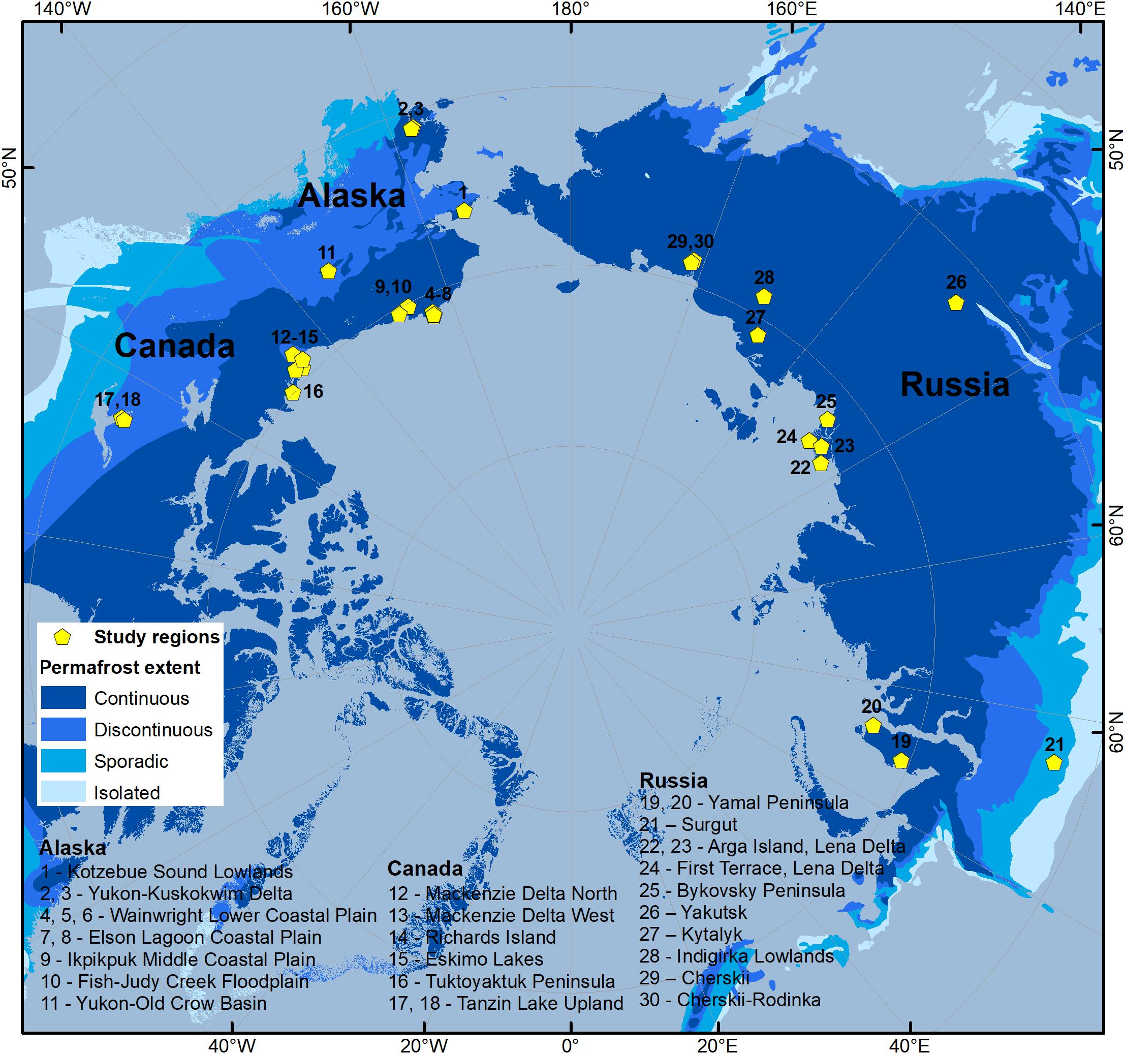
Figure 1. Location of study regions in the Arctic.

The study regions feature a great variety of waterbody types, sizes, and shapes that have formed in response to their permafrost, topographic, and geological histories (Figure 2). In terrain that was unglaciated at the time of the last glacial maximum, surface ponding occurs as a result of a combination of low topographic gradients and a near-impermeable permafrost layer. Thermal interactions between water and the frozen ground then cause further ground ice melt and subsidence, so that ponds grow both in size and depth as the underlying permafrost boundary is degraded. These thermokarst ponds and lakes are typical of the ice-rich peatlands in Russia, the Alaskan coastal plain (Figure 2c), and the coastal lowlands of Canada (Figure 2d) (Grosse et al., 2013). Here, pond and lake patterns can be either random or regular (for example, the polygonal tundra in the Lena Delta in Siberia or on the Barrow Peninsula in Alaska – Figures 2a,b). Regions such as the Canadian Shield that were glaciated during the late Pleistocene are mainly characterized by postglacial and proglacial waterbodies that typically form linear patterns (Figure 2e), which are the result of glacial scour, bedrock erosion, and glacial deposition (Shilts et al., 1987). Riverine systems such as the Mackenzie Delta in Canada, feature a highly interconnected hydrological network with flood-plains, oxbow lakes, and thermokarst ponds and lakes (Figure 2f).

FIGURE 2

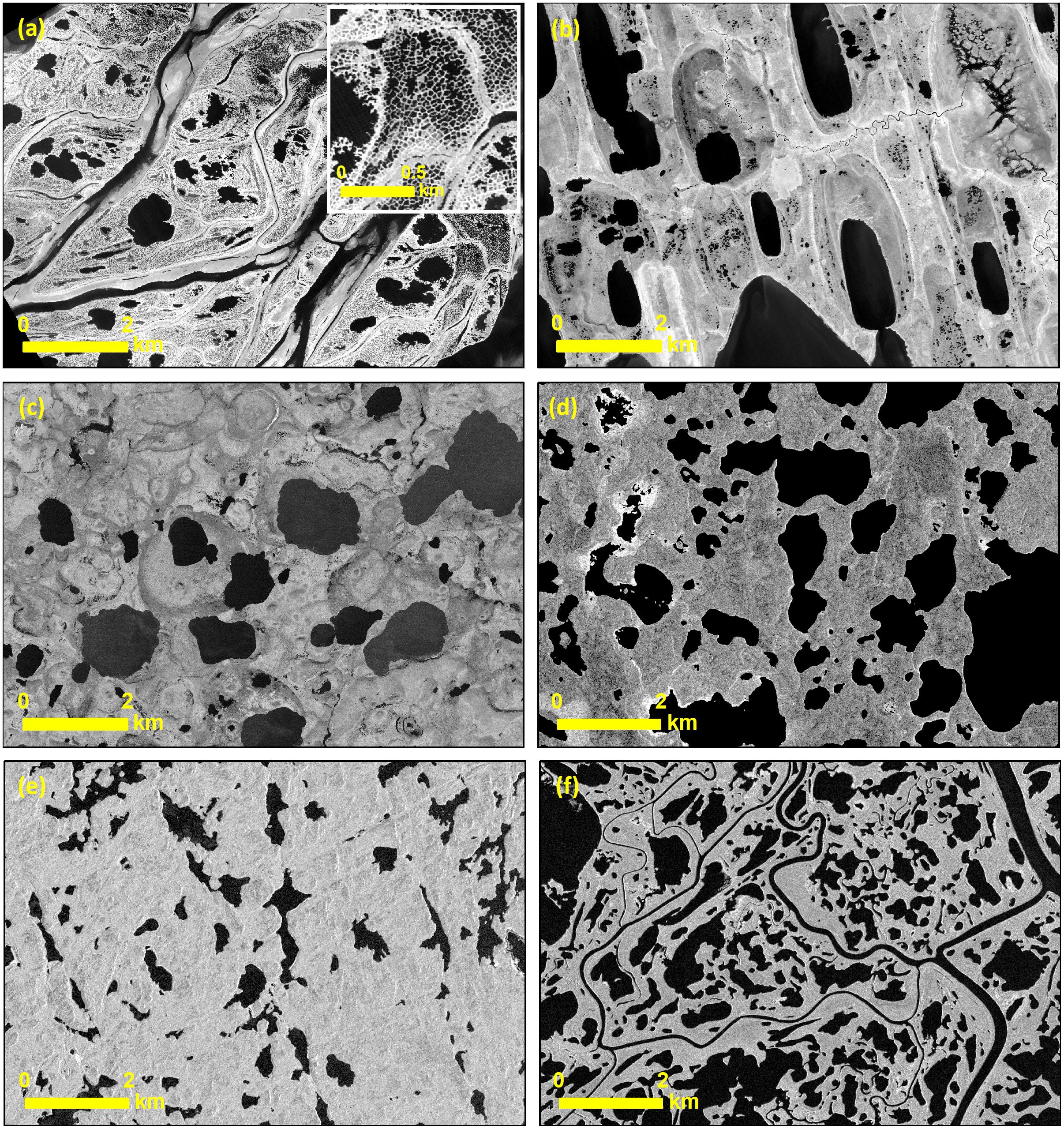
Figure 2. Waterbody patterns in different permafrost regions. (a) First terrace, Lena Delta, Russia – inset shows details of typical polygonal ponds; (b) Wainwright Lower Coastal Plain, Barrow Peninsula, Alaska; (c) Tanzin Lake Uplands, Canada; (d) Mackenzie Delta West, Canada; (e) Kotzebue Sound lowlands, Seward Peninsula, Alaska; and (f) Eskimo Lakes, Canada. Images (a,b) show the near-infrared band from KOMPSAT-2. Image (e) shows near-infrared image from SPOT-5. Images (c,d,f) are TerraSAR-X images© DLR 2013.

Materials and Methods

Preprocessing of Satellite Data and Aerial Photographs

We used waterbody maps from the PeRL database by Muster et al. (2017) for the assessment of waterbody size distributions. PeRL waterbody maps provide areas of open water. Many shallow ponds and pond or lake margins are characterized by vegetation growing or floating in the water. This type of water with vegetation could not be classified from the singleband imagery, which was the main source for PeRL classifications (Muster et al., 2017). Open water, on the other hand, can be classified confidently with high accuracy from most imagery. Accuracy of the waterbody maps ranged from 89% to more than 95% (Muster et al., 2017). Accuracy was assessed using ground surveys of lakes and ponds or aerial imagery with resolutions of less than 1 m.

For this study, we selected PeRL waterbody maps with areal extents greater than 99 km² and high classification quality. Classification quality was considered inadequate in two cases: (1) very large maps with many artifacts (e.g., shadows, rivers, streams etc.) where manual removal was not feasible and (2) manually digitized maps that could not ensure a complete account of small waterbodies. Thirty study regions were selected: 11 in Alaska, 7 in Canada, and 12 in Russia (Supplementary Table 1). Selected classifications are based on images acquired in the years between 2002 and 2013. In order to reduce the impact of inundation following snowmelt only classifications from between July and September were considered. The selected PeRL waterbody maps were derived from radar imagery (TerraSAR-X, ORRI), optical satellite imagery (Corona, GeoEye, QuickBird, WorldView-1 and -2, KOMPSAT-2), or from aerial photography. Areas of open water were extracted using a density slice or an unsupervised k-means classification in ENVI software (v4.8) on the panchromatic or near-infrared band for optical data and the X-Band (HH-polarization) for the TerraSAR-X data. Full descriptions of the image properties and the classification procedures used can be found in Muster et al. (2017). Classifications were converted from raster representations to vector representations (ESRI shape-files). The shape-files were then manually edited to remove rivers, streams, ocean in coastal areas, waterbody fragments at the image boundaries, and cloud or topographic shadows. Waterbodies smaller than 0.0001 km² – corresponding to 4 pixels at the lowest resolution of 5 m – were removed from all datasets.

Statistical Analysis

Statistics such as the areal fraction of surface water, or the mean surface area of waterbodies within a region, are meaningful measures to use for comparisons between individual study regions. However, such statistics are influenced by technical differences used to derive the waterbody maps; i.e., the remote sensing imagery used to map the waterbodies in the study regions varied in both resolution and coverage. The image resolution defines the minimum object size that can be confidently mapped while the coverage defines the maximum object size that can be captured. Limited coverage may not capture larger waterbodies even though these could be characteristic of the broader landscape. Very broad coverage, on the other hand, may reveal more variation in waterbody sizes than limited coverage. To cope with the different spatial resolutions and coverages, as well as with the wide range of waterbody sizes, we (i) band-limited the data to between 0.0001 and 1 km², and (ii) broke down study regions into boxes measuring 10 × 10 km, which were analyzed individually before averaging the statistics over the entire region.

We selected waterbodies with sizes between 0.0001 and 1 km² for our analyses. Waterbodies larger than 1 km² were excluded from the analysis because of the small sample size (10 of the 30 regions included fewer than 5 waterbodies larger than 1 km² and some of the regions had no such waterbodies). On average, waterbodies larger than 1 km² contributed less than 1% (+/–0.8 % standard deviation) to the total number of waterbodies (Figure 3).

FIGURE 3

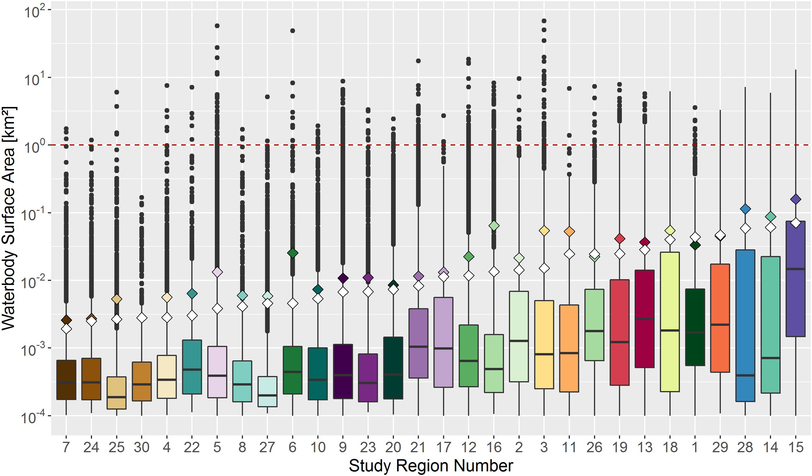
Figure 3. Boxplots of waterbody surface areas for each study region, including all waterbodies larger 0.0001 km². Study regions are sorted according to the mean size (white diamonds) calculated for waterbodies ranging between 0.0001 and 1 km² (red dashed line). Colored diamonds indicate the mean size including all waterbodies, even those with surface areas greater than 1 km². The Y-axis is plotted on a logarithmic scale. For region numbers see Figure 1 and Supplementary Table 1.

Subgrid analyses were conducted by breaking study regions into 10 × 10 km boxes. Statistics were calculated for each box and then averaged over all boxes within the study region, giving an average value for the entire region and an indication of the sub-grid heterogeneity as expressed in the standard error of the mean. A box size of 10 × 10 km was chosen as a compromise between the subgrid variability in the study region and the number of study regions for which at least four boxes could be sampled, i.e., study regions larger than about 300 km² (Muster et al., 2017). For study areas smaller than 300 km², statistics were calculated for the entire regions without any subgrid sampling.

For each study region we calculated the areal fraction of surface water of the total land area, together with the number of waterbodies per km² and the first three statistical moments (mean, variance, and skewness) of the waterbody size distribution. The variance measures how far the set of waterbody sizes are spread out from their mean. The skewness describes the extent to which the distribution is skewed toward larger (positive skewness) or smaller (negative skewness) values than the mean. For all statistical analyses we used R software (version 3.2.2).

Environmental Analysis

Each study region was described in terms of a set of climate, permafrost, and terrain variables (Supplementary Tables 2, 3), which were extracted from global or regional databases to ensure similar spatial scales for all regions (Supplementary Table 4). The climate variables included air temperature, thawing degree days (TDD), precipitation (P), evapotranspiration (ET), and precipitation minus evapotranspiration (P-ET) (Supplementary Table 2). We chose these climatic parameters because we were interested in characterizing the net water inputs across the wide range of conditions in the study regions, and the potential for long-term temperature conditions to affect waterbody size distributions. ERA-INTERIM data was used to calculate long-term averages (1979 to year of image acquisition) for the mean annual air temperature (T) as well as ET, P, and P-ET during the snow-free period. ET was derived by converting daily surface latent heat flux from Joules per m² to mm water equivalent and calculating the annual totals. We also calculated the short-term TDD, ET, P, and P-ET (i.e., for the year of image acquisition). Short-term TDD was calculated by counting all days with mean daily air temperatures larger than 0°C until the date of image acquisition. Short-term ET, P, and P-ET were calculated for the snow-free period. The start of the snow-free period for the year of image acquisition was determined to be the first day on which air temperatures of the preceding 5 days averaged more than 0.5°C. The short-term ET and P were the totals from the start of snow-free periods to the date of image acquisition. Short-term TDD and P-ET figures were used to assess the impact of seasonal variations in the water balance on the statistical moments.

The permafrost properties included its extent and ground ice content (Supplementary Table 3), as derived from regional permafrost maps. The terrain properties included average elevation and slope, derived from the GTOPO30 global DEM. Study regions were categorized as either glaciated at the time of the last glacial maximum or unglaciated at that time (Dyke et al., 2003; Hughes et al., 2016).

Kendall’s tau was used to assess correlations between variables – both between the statistical moments of the study regions and between statistical moments and environmental variables. Kendall’s tau is a non-parametric test that estimates the statistical interdependence of two datasets. If the two datasets are completely independent then the Kendall’s tau value is zero, while positive and negative values correspond to correlated and anti-correlated datasets, respectively (Kendall, 1955). A multivariate classification and regression tree (CART) analysis was also conducted in R software using the “rpart” package, in order to investigate the effect of environmental variables on the mean waterbody size, the number of waterbodies per km², the areal fraction of water, and the statistical moments.

Analyzing the Temporal Development of Waterbody Size Distributions

Change in size distributions and their moments over time were investigated using multi-decadal remote sensing data. Change detection analysis was carried out for two sites in the Kotzebue Sound Lowlands in the northern part of the Seward Peninsula, Alaska (66.3°N, 164.8°W), these being the Espenberg area (442.2 km² in extent) and the Shishmaref area (379.9 km² in extent) (Figure 3 and Supplementary Figure 1). Waterbody maps for the Espenberg area were available from Jones et al. (2011) for the years 1950/1951, 1978, and 2006/2007. Waterbody maps of the Shishmaref area were available from 1962 and 2009/2010 (Muster et al., 2017). The minimum waterbody size was set to 0.001 km², based on the resolution and image quality of the historical data (Jones et al., 2011).

Analyzing the Effect of Microtopography on Waterbody Size Distributions

In order to investigate whether or not microtopography is a dominant factor controlling waterbody size distributions we synthesized waterbody maps using a very high resolution DEM. Water was artificially added to the DEM to simulate rising water levels above the lowest elevation in the DEM (hereafter referred to as “water levels”). The imposed rising water levels progressively filled the areas from lower to higher elevations. Note that this experiment did not aim to simulate real hydrological behavior but simply to assess the effect of topography on the size distributions of waterbodies at different water levels. The DEM used was derived from airborne LiDAR data for the Fish Creek catchment area in Alaska (70.3°N, 151.2°W), acquired in July 2013 (DGGS, 2013); it had a horizontal resolution of 1 m and a vertical resolution of 0.25 m, with a vertical accuracy of 0.15 m. The selected area covered 119 km², with elevations ranging between 2.6 and 24.0 m. Waterbody maps were extracted for water levels ranging between 520 and 710 cm, at increments of 10 cm. Those DEM pixels with water levels less than or equal to the chosen water levels were extracted and converted into a vector file. All objects in the vector file with surface areas between 0.0001 and 1 km² were then treated as waterbodies and used to calculate statistical moments. This process yielded a series of maps showing continuously growing waterbodies (with increasing surface areas and depths), occupying an increasing proportion of the land area.

Results

Do Size Distributions of Arctic Waterbodies Follow a Power-Law Distribution?

We first tested whether the observed waterbody size distributions follow a power law distribution because such a relationship would be very powerful for extrapolating limited observations to larger scales. The cumulative distribution function (CDF) of a quantity with a power-law distribution appears as a straight line when plotted on logarithmic scales. We found that CDFs of waterbody sizes in our study regions did not meet this requirement (Figure 4). However, there were some straight-line relationships in the distributions over limited waterbody size ranges for a few regions (e.g., study region 21, (Figure 4B). However, these size ranges are far too small to be distinguished as power-law distributions (Newman, 2005).

FIGURE 4

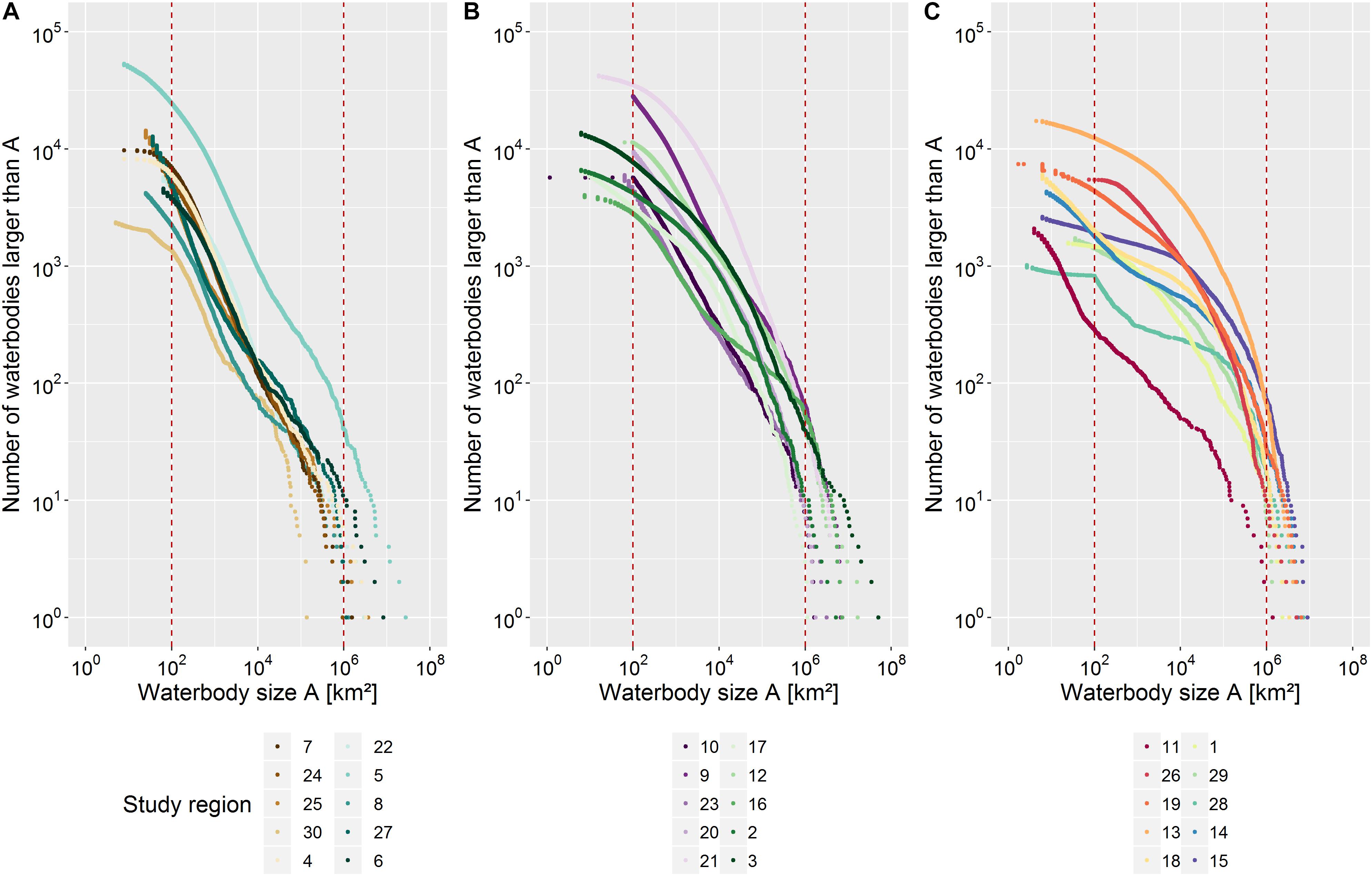
Figure 4. (A–C) A cumulative histogram or rank/frequency plot of waterbody sizes in the thirty study regions (split into three groups). Dotted lines indicate the lower and upper size limits used for the analysis (0.0001 and 1 km², respectively). Study regions are sorted according to their mean waterbodies size (within the band limit). Both the x and y axes are plotted on logarithmic scales. For study region numbers see Figure 1 and Supplementary Table 1.

Statistical Moments of Waterbody Size Distributions in Space

We found that the variance and skewness of waterbody size distributions across all of the study regions were strongly related to the mean waterbody size, i.e., the greater the mean waterbody size, the higher the variance and the lower the skewness (Figure 5 and Tables 1, 2). These relationships reflected differences in the relative proportions of small and large waterbodies: study regions in which the waterbodies had a small mean size are characterized by many small waterbodies and few large ones, in contrast to regions in which the waterbodies had a larger mean surface area, where larger waterbodies are more common. For example, the Elson Lagoon Coastal Plain in Alaska (study region #7) was characterized by polygonal tundra with many small ponds. Waterbodies in this region had a mean waterbody size of 0.0019 km² and a small variance of 0.0004 km⁴. The size distribution was heavily right-skewed with a skewness of 28.6 and 92% of the waterbodies being smaller than the mean. This predominance of small waterbodies could be seen in the region’s PDF, which had a peak to the left of the mean (Figures 6A,B). A small number of waterbodies were much larger than the average waterbody, which produces the long tail to the right of the PDF. The probability of waterbodies on the Elson Lagoon coastal plain being larger than, for example, 0.01 km² was therefore very low. Looking at the all size distributions and their statistical moments, the greater the mean waterbody size in a study region is, the higher is the probability of it containing waterbodies larger than 0.01 km². The Eskimo Lakes region (# 15) in Canada had the highest mean waterbody size of all the regions investigated (0.0709 km²; Figure 5 and Table 1). About half of the waterbodies in this region had sizes larger than 0.01 km² and the region’s waterbody size distribution had a high variance (0.0219 km⁴) but a low skewness (3.3), as the waterbody sizes were more evenly distributed around the mean (Figure 6C). This region included both more relatively large waterbodies than the Elson Lagoon coastal plain and a larger range of waterbody sizes. Three of the regions – Eskimo Lakes (# 15), Tanzin Lake Uplands (#18), and Indigirka Lowlands (#28) – had a bimodal distribution (Figure 6C). The bimodality is not visible on the waterbody maps, i.e., no subregions with different size distributions are discernible. Although the shape of the distributions is different for those regions, the corresponding data points are still on the curve representing all regions (Figure 4). Reasons for the bimodality in these three regions are unclear, motivating future analyses of these systems.

FIGURE 5

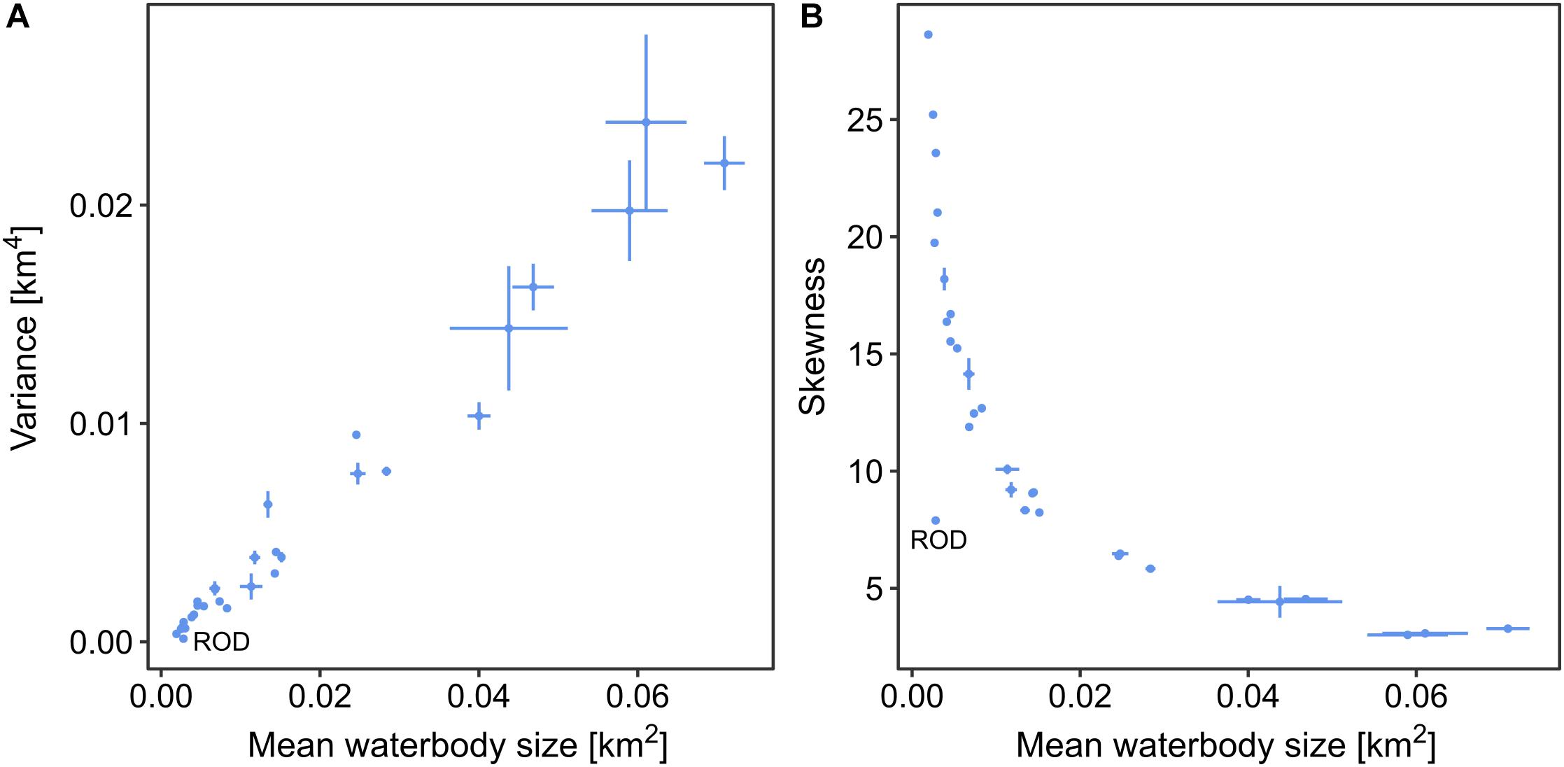
Figure 5. Variations in the statistical moments of waterbody size distributions of the 30 Arctic study regions. The variance (A) and skewness (B) of the size distributions for each study region are plotted against the mean waterbody size. The moments are calculated for waterbodies with sizes between 0.0001 and 1 km². The vertical and horizontal bars represent the standard deviation of the means of the mean size, variance, and skewness across 10 × 10 km subsets of the larger study regions (i.e., those covering 300 km² or more). The size distribution for waterbodies in the Cherskii-Rodinka region (ROD) is significantly less skewed than those for other regions with comparable mean waterbody sizes.

TABLE 1

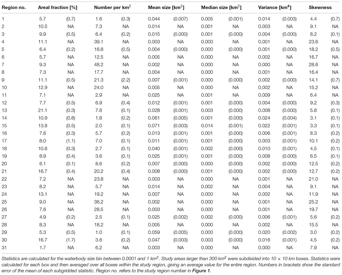
Table 1. Statistics of waterbody size distributions for each region.

TABLE 2

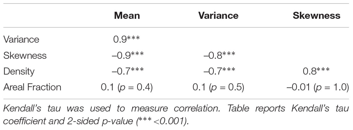
Table 2. Correlation matrix of distribution statistics.

FIGURE 6

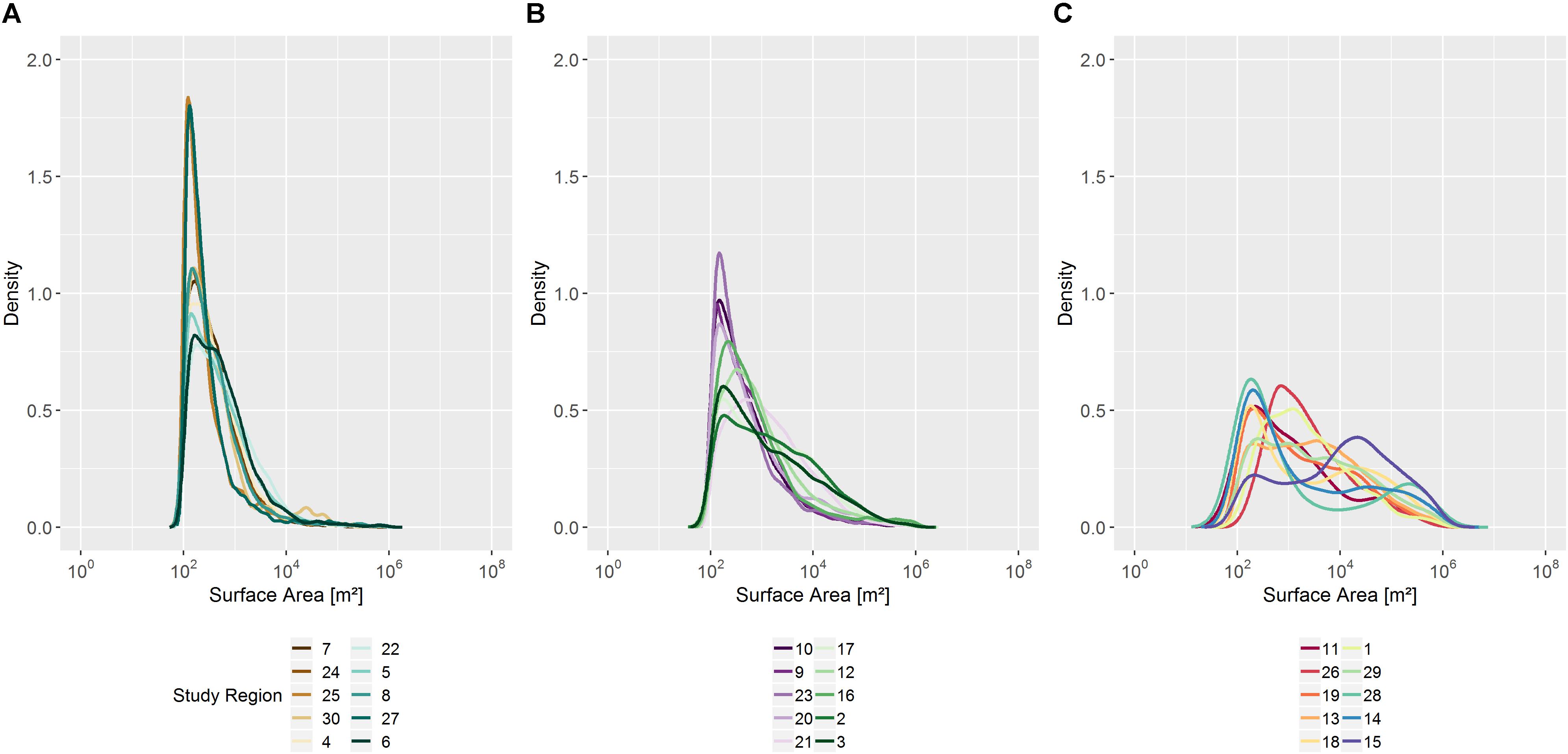
Figure 6. (A–C) Probability density functions (PDF) for band-limited (0.0001 to 1 km²) waterbody size distributions, for three groups of ten study regions. The X-axis is plotted on a logarithmic scale; the PDFs were calculated from log-transformed data. Study regions are sorted according to their mean waterbody sizes. For region numbers see Figure 1 and Supplementary Table 1.

The mean waterbody size did correlate with the number of waterbodies per km² (Supplementary Figure 4B). However, neither the number of waterbodies nor the mean waterbody size did correlate with the areal fraction of surface water (Supplementary Figures 4A,C). We also did not find any significant correlations between the statistical moments and environmental factors (Supplementary Figures 2, 3). The highest Kendall’s tau value (0.45) was found between long-term P-ET values and mean waterbody sizes (Table 3). It is interesting, however, to note that there was one exception, the Cherskii-Rodinka region (#30) in north-eastern Siberia, which had a relatively small mean waterbody size (0.0028 km²) but a waterbody size distribution that was not as highly skewed as those of other regions with similar mean waterbody sizes. This region has a significantly different topography from all of the other regions investigated, with higher elevations and steeper slopes (Supplementary Table 3).

TABLE 3

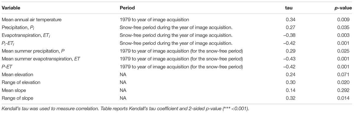
Table 3. Correlation matrix of mean waterbody size versus environmental variables.

Statistical Moments of Waterbody Size Distributions Over Time

Multi-decadal imagery between 1962 and 2010 shows significant drying of the Shishmaref study area on the Seward Peninsula in terms of a reduction in both the number of waterbodies and the areal fraction of surface water (Table 4). However, the changes to waterbodies over time were diverse; they included the development of new waterbodies, the coalescence of adjacent waterbodies, and either complete or partial drainage of existing waterbodies (Figure 7). The size distribution shifted from smaller to larger waterbodies and the mean waterbody size increased. In 1962, 74% of the waterbodies were smaller than 0.01 km² but in 2010 they had decreased to 58%. This change was accompanied by an increase in the variance in waterbody sizes and a more even distribution of their sizes around the mean, i.e., a reduction in skewness. Changes in the Espenberg area were less pronounced (Table 4). Nonetheless, the temporal changes in the statistical moments from the waterbody size distributions of both the Shishmaref and Espenberg areas matched the variations in statistical moments of waterbody size distributions for the 30 study regions (Figure 8).

TABLE 4

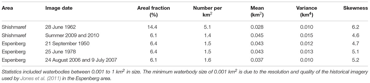
Table 4. Statistics of waterbody size distributions over time for Shishmaref and Espenberg areas in the Kotzebue Sound Lowlands, Alaska.

FIGURE 7

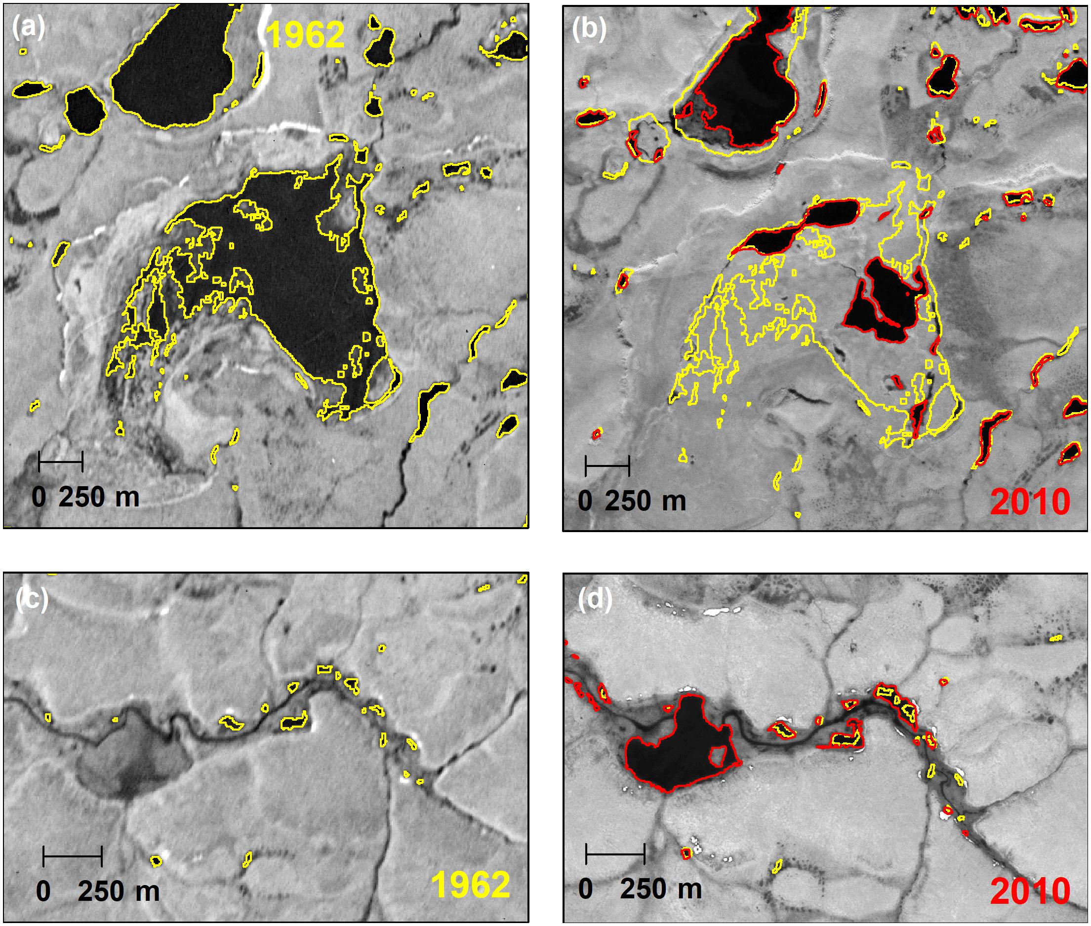
Figure 7. Temporal changes of waterbody sizes in the Shishmaref area in the Kotzebue Sound Lowlands (study region #1) of the Seward Peninsula, Alaska. Waterbody outlines are marked in yellow for 1962 and in red outlines for 2010: (a) and (b) illustrate complete and partial drainage of waterbodies, while (c) and (d) illustrate waterbody formation and expansion.

FIGURE 8

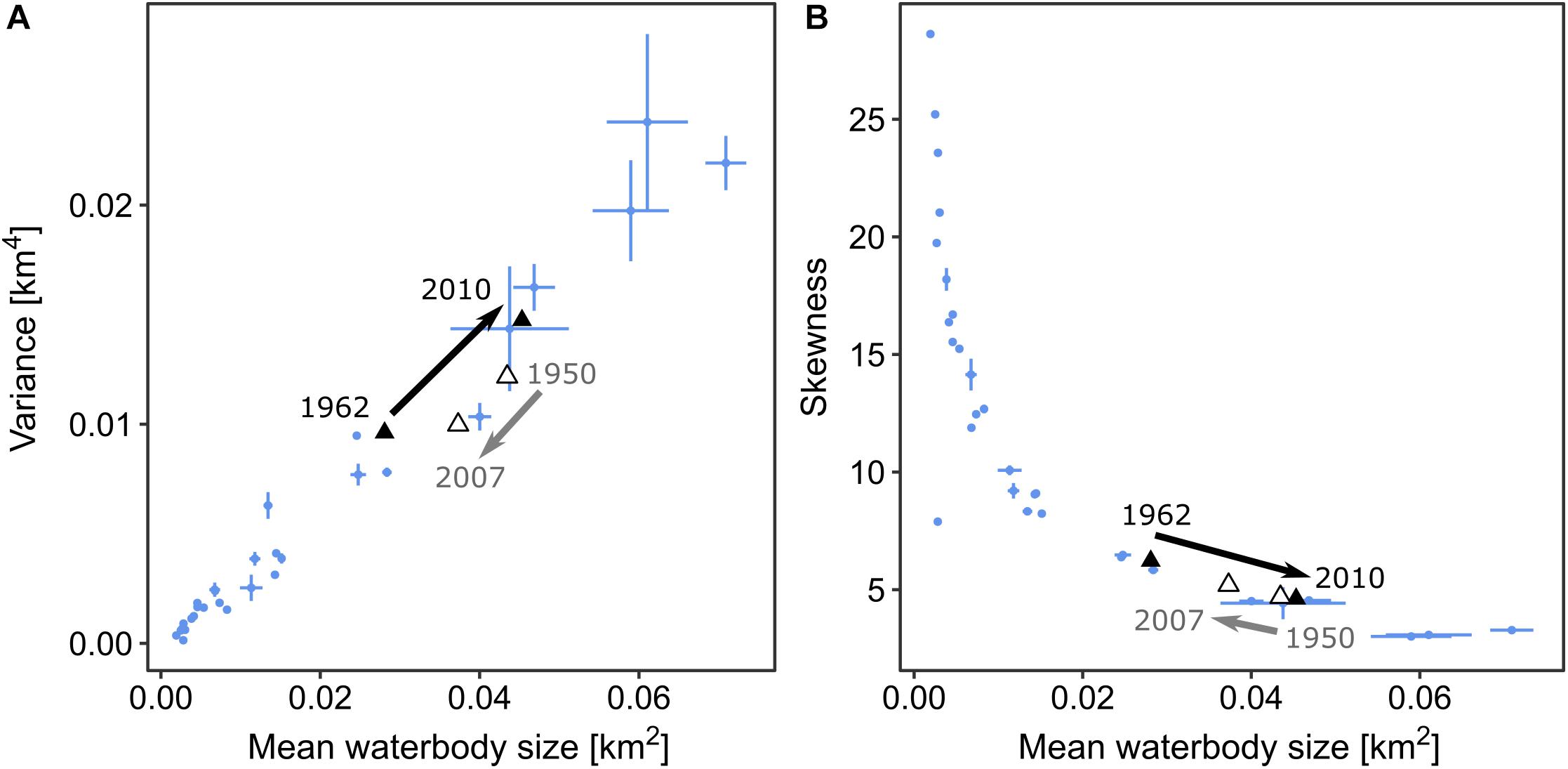
Figure 8. Variations in the statistical moments of waterbody size distributions over time. The triangles and arrows indicate the development of statistical moments for the Shishmaref (black triangles: 1962–2010) and Espenberg areas (white triangles: 1950–2007) in the Kotzebue Sound Lowlands on the Seward Peninsula, for waterbody sizes between 0.001 and 1 km². Blue points indicate the variance (A) and skewness (B) of the size distributions for each study region against the mean waterbody size.

DEM Filling Exercise

To further explore the observed relationships of statistical moments we performed numerical experiments for the Fish Creek region in Alaska, using a high-resolution DEM (Figure 9). These experiments involved estimating the waterbody sizes purely on the basis of topography, ignoring surface and sub-surface water flows. Increases in the mean waterbody size were accompanied by an increase in variance and a decrease in skewness – similar to the observed relationships across the 30 study regions. Statistical moments of waterbody size distributions from both the real and synthetic waterbody maps correlated with the density of waterbodies (i.e., with the number of waterbodies per km²) but not with the areal fraction of surface water. We would intuitively have expected increasingly large waterbodies as the water levels increased and a corresponding increase in mean waterbody size. While this is the case in some areas, the formation of small waterbodies depends on the microtopography, which can be found on different topographic levels. For example, the selected DEM profile (Figure 9a) can be subdivided into two general areas: a lower level from about to 6.6 to 6.8 m a.s.l. and a higher level from about 6.9 to 7.4 m a.s.l. With increasing water levels small ponds first form in the lower level area and eventually merge into one large waterbody. However, when the water level reaches the higher level area many new ponds form. Although the areal fraction is growing continuously, the addition of these small waterbodies to the size distribution reduces the mean waterbody size.

FIGURE 9

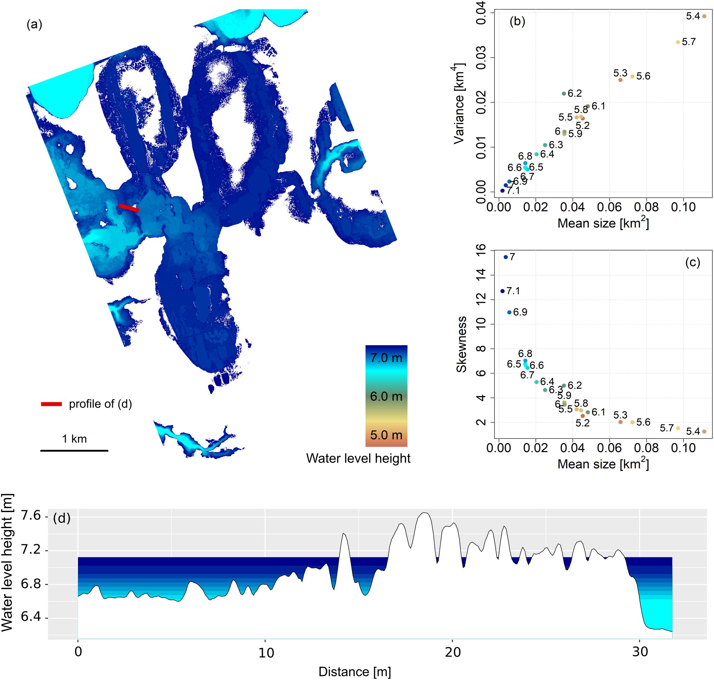
Figure 9. Synthetic waterbody map, together with statistical moments for the waterbody size distributions, for the Fish Creek catchment area, Alaska. (a) Synthetic waterbody map; different colors indicate the different water levels at which waterbodies were extracted. Plots of the variance (b) and skewness (c) of waterbody size distributions versus mean waterbody size: the point colors correspond to the colors on the map and the labels refer to the surface water levels in meters above sea level. Those DEM pixels elevations lower than or equal to the chosen water level were extracted and converted into a vector file. This method produced a series of waterbody maps with continuously growing and deepening waterbodies. The section (d) is a DEM profile that illustrates the increase in water level (red line on the map marks the position of the DEM profile).

Discussion

We found three pieces of evidence suggesting the existence of consistent controls for waterbody size distributions in lowland permafrost landscapes. First, strong relationships were found between the mean and variance of waterbody sizes and between the mean and skewness of waterbody sizes across thirty permafrost landscapes. Second, observed temporal changes in waterbody size distributions on the Seward Peninsula and their associated statistical moments aligned with the observed spatial relationships between statistical moments across the 30 study regions. Third, we reproduced the observed relationships between the statistical moments by extracting synthetic waterbody distributions for different water levels from a high-resolution DEM.

Statistical Moments of Waterbody Size Distributions of Different Arctic Regions

We found a clear relationship between the statistical moments of waterbody size distributions across our study regions. Each study region has a different proportion of small and large waterbodies and the different proportions in each study region correspond to different mean waterbody sizes. Across regions, the mean waterbody size is related to the variance (the width of the size distribution) and skewness.

The relationships of statistical moments hold across a broad range of landscapes with varying hydrology, climate, permafrost and topography, suggesting similar underlying controls across study regions. Our analysis found that the observed mean-variance and mean-skewness relationships could not be explained by hydrological variables such as TDD s, evapotranspiration, precipitation, permafrost extent, glaciation history, or broad-scale topographic parameters (i.e., elevation and slope). This may be due to data uncertainty in the large-scale environmental variables we used for analysis. However, our study looked at snapshots of different landscapes, in presumably different states, not at a time series of one landscape. Finding the observed universal relationships thus suggests that the underlying landscapes are structurally similar. Our simple DEM filling exercise produced waterbody distributions with very similar mean-variance and mean-skewness relationships to those observed across the Arctic. This result illustrates how the relationships between moments are tightly linked to the landscape topography. Most of the study regions are quite flat, with mean gradients of less than 1°, so that the distribution of water in the landscape is mainly controlled by microtopography (Woo and Guan, 2006; Boike et al., 2008; Helbig et al., 2013; Liljedahl et al., 2016). The only exception is the Cherskii-Rodinka study region which has a significantly higher mean slope of 2.1° than all other regions and does not fall on the observed mean-skewness relationship. The particular shape of the mean-variance and mean-skewness relationships is another indicator that the distributions do not follow a power law. If the size distribution of waterbodies followed a universal power law (as described in section 4.1), the variance would increase in proportion to the square of the mean. However, no such relationship was observed. Instead, we suggest that a trade-off between the number and size of waterbodies is responsible for the particular shape of the mean-variance and mean-skewness relationships. Waterbodies cannot form and grow unobstructed in a landscape. For example, in a topographic depression with many small waterbodies the growth of one or more of these waterbodies would result in coalescence, which would increase the sizes of the waterbodies while reducing their number. Conversely, when a large waterbody begins to dry or empty, several smaller waterbodies may remain so that the number of waterbodies increase but the average size decreases. In the case of the coalescence of waterbodies, for example, we deduce that smaller waterbodies disappear more rapidly than new larger waterbodies are formed, causing the mean waterbody size and variance to increase linearly and the skewness to decrease.

Statistical Moments of Waterbody Size Distributions Over Time

The above described spatial trade-off of waterbody loss and growth may occur simultaneously at different sites within the same region as seen at the Espenberg and Shishmaref sites on the Northern Seward Peninsula where we had multi-decadal imagery. This study did not investigate the reasons for the shifts in waterbody size distributions on the Northern Seward Peninsula. Jones et al. (2011), however, did conduct a detailed investigation of lake dynamics in at the Espenberg site and found that the majority of thermokarst lakes at the site are actively expanding because of surface permafrost degradation and may eventually drain when they encroach the drainage gradient. Similar processes are likely responsible for the observed changes in waterbody sizes in the Shishmaref area, which is located within the same region as the Espenberg area. Changes in waterbody sizes can result from changes in the water balance, changes in the topography, or a combination of both. In a thermokarst system, for example, ground ice melt causes the land surface to subside which in turn changes the hydrodynamics of the landscape (Jorgenson and Shur, 2007; Liljedahl et al., 2016). In landscapes not dominated by thermokarst processes, waterbody area dynamics are more likely affected by climate than by changes in topography or storage capacity (Karlsson et al., 2015). In general, changes in climate, water balance, or topography affect waterbodies of all sizes and may cause diverse trends of waterbodies shrinking and growing (Smol and Douglas, 2007; Carroll et al., 2011; Watts et al., 2012; Andresen and Lougheed, 2015; Boike et al., 2016; Liljedahl et al., 2016; Carroll and Loboda, 2017). The dominant process would then determine the direction and magnitude of the shift in the size distribution (Karlsson et al., 2014; Carroll and Loboda, 2017). We note that small waterbodies can show a strong response to seasonal changes in water output and input between years and even within the same year (Bowling et al., 2003; Boike et al., 2008; Abnizova and Young, 2010). We were not able to analyze in this study the effects of seasonality due to a lack of sufficient data. In large study regions, however, variability in waterbody size distributions over time can be due to a combination of short-term variability in local water balance and long-term geomorphological dynamics (Chen et al., 2014). As observed in other studies throughout the Arctic, mechanisms, spatial variation, and time scales of change can be diverse even within the same region due to spatial variation of lake types, and varying hydrologic and geomorphic processes within a region (Riordan et al., 2006; Jones et al., 2011; Roach et al., 2011; Arp et al., 2011).

Outlook on Future Research and Potential Applications

The consistency of the observed mean-variance and mean-skewness relationships between the statistical moments over space and time strongly suggest predictable patterns in waterbody size distributions. The relationships establish spatial and temporal constraints on the range of size distributions in space and time. The prediction of the direction and rate of change as well as the reasons for change, however, remain to be investigated in individual landscape studies.

The temporal pattern could only be demonstrated at two sites where sufficient data was available. However, more than two observations would obviously be required to corroborate this suggestion further. Similarly, the effect of topography should be explored further. The observed relationships comprise landscapes with a very flat topography, although the single outlier region hints at more complicated structures that may be expected to appear as the range of landscapes and topographic systems are extended. To adequately capture the effect of topography, high-resolution DEMs are needed. For example, LIDAR data with a vertical resolution of 1 m or less would facilitate detailed analyses of relationships between topography and waterbody size distributions across the Arctic.

The identified relationships are likely to be of great value in modeling applications. While very large waterbodies have been well represented in models, smaller waterbodies have not. The computational constraints of present-day large-scale models preclude the use of information on individual waterbodies, such as their properties and locations. Statistical or reduced-order model representations are therefore used instead to facilitate land-surface observational modeling and data assimilation (Ji et al., 2015; Pau et al., 2016). Under the constraints and limitations discussed above, the variance-mean and skewness-mean relationships provide valuable constraints for generating waterbody size distributions on a subgrid scale and allow the evaluations of hydrological and land surface modeling outcome.

Conclusion

In this study we have, for the first time, investigated size distributions of Arctic waterbodies with sizes as small as 0.0001 km² (100 m²). We focused on thirty permafrost lowland regions in the Arctic, which represent a cross-section of the main Arctic lake regions and dominant waterbody types. These waterbody size distributions were not representable by a power law so that simple extrapolations from coarse-scale observations were not possible. Nevertheless, we found three pieces of evidence suggesting consistent spatial and temporal controls on the observed waterbody size distributions. First, we found relationships between the mean and variance and the mean and skewness of the observed waterbody size distributions. Second, we showed that these relationships persisted over time in the two areas for which high-resolution multi-decadal imagery was available. Third, these relationships emerge in synthetic waterbody distributions established using different surface water levels in a high-resolution DEM, illustrating that the moments are tightly coupled with the landscape’s topography. We suggest that these properties will be of great value when simulating size distributions of waterbodies for a range of Arctic spatial scales and landscapes. The relationships between the statistical moments of the waterbody size distributions have potentially far-reaching implications for attempts to predict the distribution and development of waterbody-dominated landscapes in the Arctic because they constrain possible variations in space and over time. In particular, we note that these size distributions can be used to generate sub-grid parameterizations of small waterbodies in large-scale models and thus fill an important gap in the understanding of the Arctic’s future hydrological and biogeochemical dynamics.

Data Availability

The datasets analyzed for this study can be found in the PANGAEA repository: https://doi.pangaea.de/10.1594/PANGAEA.868349.

Author Contributions

All authors listed have made a substantial, direct and intellectual contribution to the work, and approved it for publication.

Funding

This work was supported by the Helmholtz Association through a grant (VH-NG 203) awarded to SM, WR, CK, and CW were supported by the US Department of Energy’s BER program under the NGEE-Arctic project (contract no. DE-AC02-05CH11231). GG was supported by the European Research Council (ERC) grant no. 338335. Any use of trade, product, or firm names is for descriptive purposes only and does not imply endorsement by the US Government. BJ was supported by the National Science Foundation under grant OPP-1806213.

Conflict of Interest Statement

The authors declare that the research was conducted in the absence of any commercial or financial relationships that could be construed as a potential conflict of interest.

Acknowledgments

All TerraSAR-X data were made available by the German Aerospace Center (DLR) through PI agreement LAN1747, within the framework of the European Space Agency (ESA) funded DUE Permafrost project, the EU FP7 PAGE21 project, and the Austrian-Russian joint FWF COLD Yamal project (I 1401). KOMPSAT data were provided by the European Space Agency (ESA) to the ACCOnet Project (International Polar Year AO Project 4133). GTOPO 30 data is available from the U.S. Geological Survey.

Supplementary Material

The Supplementary Material for this article can be found online at: https://www.frontiersin.org/articles/10.3389/feart.2019.00005/full#supplementary-material

References

Abnizova, A., Siemens, J., Langer, M., and Boike, J. (2012). Small ponds with major impact: the relevance of ponds and lakes in permafrost landscapes to carbon dioxide emissions. Global Biogeochem. Cycles 26:GB2041. doi: 10.1029/2011gb004237

CrossRef Full Text | Google Scholar

Abnizova, A., and Young, K. L. (2010). Sustainability of High Arctic ponds in a polar desert environment. Arctic 63, 67–84. doi: 10.14430/arctic648

CrossRef Full Text | Google Scholar

Andresen, C. G., and Lougheed, V. L. (2015). Disappearing Arctic tundra ponds: fine-scale analysis of surface hydrology in drained thaw lake basins over a 65 year period (1948–2013). J. Geophys. Res. Biogeo. 120, 466–479. doi: 10.1002/2014JG002778

CrossRef Full Text | Google Scholar

Anthony, K. W., von Deimling, T. S., Nitze, I., Frolking, S., Emond, A., Daanen, R., et al. (2018). 21st-century modeled permafrost carbon emissions accelerated by abrupt thaw beneath lakes. Nat. Commun. 9:3262. doi: 10.1038/s41467-018-05738-9

PubMed Abstract | CrossRef Full Text | Google Scholar

Arp, C. D., Jones, B. M., Urban, F. E., and Grosse, G. (2011). Hydrogeomorphic processes of thermokarst lakes with grounded-ice and floating-ice regimes on the Arctic Coastal Plain, Alaska. Hydrol. Process. 25, 2422–2438. doi: 10.1002/hyp.8019

CrossRef Full Text | Google Scholar

Avis, C. A., Weaver, A. J., and Meissner, K. J. (2011). Reduction in areal extent of high-latitude wetlands in response to permafrost thaw. Nat. Geosci. 4, 444–448. doi: 10.1038/NGEO1160

CrossRef Full Text | Google Scholar

Boike, J., Grau, T., Heim, B., Günther, F., Langer, M., Muster, S., et al. (2016). Satellite-derived changes in the permafrost landscape of central Yakutia,2000–2011: wetting, drying, and fires. Glob. Planet. Change 139, 116–127. doi: 10.1016/j.gloplacha.2016.01.001

CrossRef Full Text | Google Scholar

Boike, J., Wille, C., and Abnizova, A. (2008). Climatology and summer energy and water balance of polygonal tundra in the Lena River Delta, Siberia. J. Geophys. Res. Biogeosci. 113, G03025. doi: 10.1029/2007JG000540

CrossRef Full Text | Google Scholar

Bowling, L. C., Kane, D. L., Gieck, R. E., Hinzman, L. D., and Lettenmaier, D. P. (2003). The role of surface storage in a low-gradient arctic watershed. Water Resour. Res. 39:1087. doi: 10.1029/2002WR001466

CrossRef Full Text | Google Scholar

Brocca, L., Morbidelli, R., Melone, F., and Moramarco, T. (2007). Soil moisture spatial variability in experimental areas of central Italy. J. Hydrol. 333, 356–373. doi: 10.1016/j.jhydrol.2006.09.004

CrossRef Full Text | Google Scholar

Carroll, M., and Loboda, T. (2017). Multi-decadal surface water dynamics in north american tundra. Remote Sens. 9:497. doi: 10.3390/rs9050497

CrossRef Full Text | Google Scholar

Carroll, M., Townshend, J., DiMiceli, C., Loboda, T., and Sohlberg, R. (2011). Shrinking lakes of the arctic: spatial relationships and trajectory of change. Geophys. Res. Lett. 38:L20406. doi: 10.1029/2011GL049427

CrossRef Full Text | Google Scholar

Chen, M., Rowland, J. C., Wilson, C. J., Altmann, G. L., and Brumby, S. P. (2014). Temporal and spatial pattern of thermokarst lake area changes at Yukon Flats, Alaska. Hydrol. Process. 28, 837–852. doi: 10.1002/hyp.9642

CrossRef Full Text | Google Scholar

DGGS (2013). Elevation Datasets of Alaska, Edited by Alaska Division of Geological & Geophysical Surveys Digital Data Series 4. Available at: http://maps.dggs.alaska.gov/elevationdata/

Downing, J. A., Prairie, Y. T., Cole, J. J., Duarte, C. M., Tranvik, L. J., Striegl, R. G., et al. (2006). The global abundance and size distribution of lakes, ponds, and impoundments. Limnol. Oceanogr. 51, 2388–2397. doi: 10.4319/lo.2006.51.5.2388

CrossRef Full Text | Google Scholar

Dyke, A. S., Moore, A., and Robertson, L. (2003). Deglaciation of North America, Geological Survey of Canada Ottawa. Open File 1574. Ottawa: Natural Resources Canada, doi: 10.4095/214399

CrossRef Full Text | Google Scholar

Famiglietti, J. S., Rudnicki, J. W., and Rodell, M. (1998). Variability in surface moisture content along a hillslope transect: rattlesnake hill, texas. J. Hydrol. 210, 259–281. doi: 10.1016/S0022-1694(98)00187-5

CrossRef Full Text | Google Scholar

Folk, R. L., and Ward, W. C. (1957). Brazos river bar: a study in the significance of grain size parameters. J. Sediment. Res. 27, 3–26. doi: 10.1306/74D70646-2B21-11D7-8648000102C1865D

CrossRef Full Text | Google Scholar

Grosse, G., Jones, B., and Arp, C. D. (2013). Thermokarst lakes, drainage, and drained basins. Treatise Geomorphol. 8:29. doi: 10.1016/B978-0-12-374739-6.00216-5

CrossRef Full Text | Google Scholar

Helbig, M., Boike, J., Langer, M., Schreiber, P., Runkle, B. R., and Kutzbach, L. (2013). Spatial and seasonal variability of polygonal tundra water balance: Lena River Delta, northern Siberia (Russia). Hydrogeol. J. 21, 133–147. doi: 10.1007/s10040-012-0933-4

CrossRef Full Text | Google Scholar

Hu, Z., Islam, S., and Cheng, Y. (1997). Statistical characterization of remotely sensed soil moisture images. Remote Sens. Environ. 61, 310–318. doi: 10.1016/S0034-4257(97)89498-9

CrossRef Full Text | Google Scholar

Hughes, A. L. C., Gyllencreutz, R., Lohne,Ø. S., Mangerud, J., and Svendsen, J. I (2016). The last Eurasian ice sheets–a chronological database and time-slice reconstruction, DATED1. Boreas 45, 1–45. doi: 10.1111/bor.12142

CrossRef Full Text | Google Scholar

Ji, X., Shen, C., and Riley, W. J. (2015). Temporal evolution of soil moisture statistical fractal and controls by soil texture and regional groundwater flow. Adv. Water Resour. 86, 155–169. doi: 10.1016/j.advwatres.2015.09.027

CrossRef Full Text | Google Scholar

Jones, B. M., Grosse, G., Arp, C. D., Jones, M. C., Anthony, K. M. W., and Romanovsky, V. E. (2011). Modern thermokarstlake dynamics in the continuous permafrost zone, northern Seward Peninsula. Alaska, J. Geophys. Res. 116:G00M03. doi: 10.1029/2011JG001666

CrossRef Full Text

Jorgenson, M., Yoshikawa, K., Kanevskiy, M., Shur, Y., Romanovsky, V., Marchenko, S., et al. (2008). Permafrost characteristics of Alaska. Proc. Ninth Int. Conference Permafrost 3, 121–122.

Google Scholar

Jorgenson, M. T., and Shur, Y. (2007). Evolution of lakes and basins in northern Alaska and discussion of the thaw lake cycle. J. Geophys. Res. Earth Surf. 112:F02S17. doi: 10.1029/2006JF000531

CrossRef Full Text | Google Scholar

Jun, C., Ban, Y., and Li, S. (2014). China: Open access to Earth land-cover map. Nature 514, 434–434. doi: 10.1038/514434c

PubMed Abstract | CrossRef Full Text | Google Scholar

Karlsson, J. M., Jaramillo, F., and Destouni, G. (2015). Hydro-climatic and lake change patterns in Arctic permafrost and non-permafrost areas. J. Hydrol. 529, 134–145. doi: 10.1016/j.jhydrol.2015.07.005

CrossRef Full Text | Google Scholar

Karlsson, J. M., Lyon, S. W., and Destouni, G. (2014). Temporal behavior of lake size-distribution in a thawing permafrost landscape in northwestern Siberia. Remote Sens. 6, 621–636. doi: 10.3390/rs6010621

CrossRef Full Text | Google Scholar

Kastowski, M., Hinderer, M., and Vecsei, A. (2011). Long-term carbon burial in European lakes: Analysis and estimate. Global Biogeochem. Cycles 25:GB3019. doi: 10.1029/2010GB003874

CrossRef Full Text | Google Scholar

Kendall, M. G. (1955). Rank Correlation Methods. New York, NY: Hafner Publishing Co.

Google Scholar

Langer, M., Westermann, S., Anthony, K. W., Wischnewski, K., and Boike, J. (2015). Frozen ponds: production and storage of methane during the Arctic winter in a lowland tundra landscape in northern Siberia. Lena River delta. Biogeosciences 12, 977–990. doi: 10.5194/bg-12-977-2015

CrossRef Full Text | Google Scholar

Langer, M., Westermann, S., Boike, J., Kirillin, G., Grosse, G., Peng, S., et al. (2016). Rapid degradation of permafrost underneath waterbodies in tundra landscapes—toward a representation of thermokarst in land surface models. J. Geophys. Res. 121, 2446–2470. doi: 10.1002/2016JF003956

CrossRef Full Text | Google Scholar

Laurion, I., Vincent, W. F., MacIntyre, S., Retamal, L., Dupont, C., Francus, P., et al. (2010). Variability in greenhouse gas emissions from permafrost thaw ponds. Limnol. Oceanogr. 55, 115–133. doi: 10.4319/lo.2010.55.1.0115

CrossRef Full Text | Google Scholar

Lehner, B., and Döll, P. (2004). Development and validation of a global database of lakes, reservoirs and wetlands. J. Hydrol. 296, 1–22. doi: 10.1016/j.jhydrol.2004.03.028

CrossRef Full Text | Google Scholar

Lewis, W. M. Jr. (2011). Global primary production of lakes: 19th Baldi Memorial Lecture. Inland Waters 1, 1–28. doi: 10.5268/IW-1.1.384

CrossRef Full Text | Google Scholar

Li, B., and Rodell, M. (2013). Spatial variability and its scale dependency of observed and modeled soil moisture over different climate regions. Hydrol. Earth Syst. Sci. 17, 1177–1188. doi: 10.5194/hess-17-1177-2013

CrossRef Full Text | Google Scholar

Liljedahl, A. K., Boike, J., Daanen Ronald, P., Fedorov Alexander, N., Frost Gerald, V., Grosse, G., et al. (2016). Pan-Arctic ice-wedge degradation in warming permafrost and its influence on tundra hydrology. Nat. Geosci. 9, 312–318. doi: 10.1038/ngeo2674

CrossRef Full Text | Google Scholar

Marshall, I. B., and Schut, P. (1999). A National Ecological Framework for Canada. Ottawa, ON: Agriculture and Agri-Food Canada.

Google Scholar

McGuire, A. D., Anderson, L. G., Christensen, T. R., Dallimore, S., Guo, L., Hayes, D. J., et al. (2009). Sensitivity of the carbon cycle in the arctic to climate change. Ecol. Monogr. 79, 523–555. doi: 10.1890/08-2025.1

CrossRef Full Text | Google Scholar

McLaren, P., and Bowles, D. (1985). The effects of sediment transport on grain-size distributions. J. Sediment. Res. 55, 457–470.

Google Scholar

Muster, S., Heim, B., Abnizova, A., and Boike, J. (2013). Water body distributions across scales: a remote sensing based comparison of three Arctic tundra wetlands. Remote Sens. 5, 1498–1523. doi: 10.3390/rs5041498

CrossRef Full Text | Google Scholar

Muster, S., Roth, K., Langer, M., Lange, S., Cresto Aleina, F., Bartsch, A., et al. (2017). PeRL: a circum-arctic permafrost region pond and Lake database. Earth Syst. Sci. Data 9, 317–334. doi: 10.1111/gcb.14289

PubMed Abstract | CrossRef Full Text | Google Scholar

Newman, M. E. J. (2005). Power laws, pareto distributions and Zipf’s law. Contemp. Phys. 46, 323–351. doi: 10.1080/00107510500052444

CrossRef Full Text | Google Scholar

Paltan, H., Dash, J., and Edwards, M. (2015). A refined mapping of Arctic lakes using Landsat imagery. Int. J. Remote Sens. 36, 5970–5982. doi: 10.1080/01431161.2015.1110263

CrossRef Full Text | Google Scholar

Papa, F., Prigent, C., Aires, F., Jimenez, C., Rossow, W., and Matthews, E. (2010). Interannual variability of surface water extent at the global scale. 1993–2004. J. Geophys. Res. Atmos. 115, D12111. doi: 10.1029/2009JD012674

CrossRef Full Text | Google Scholar

Pau, G. S. H., Shen, C., Riley, W. J., and Liu, Y. (2016). Accurate and efficient prediction of fine-resolution hydrologic and carbon dynamic simulations from coarse-resolution models. Water Resour. Res. 52, 791–812. doi: 10.1002/2015WR017782

CrossRef Full Text | Google Scholar

Pekel, J.-F., Cottam, A., Gorelick, N., and Belward, A. S. (2016). High-resolution mapping of global surface water and its long-term changes. Nature 540,418–422. doi: 10.1038/nature20584

PubMed Abstract | CrossRef Full Text | Google Scholar

Rautio, M., Dufresne, F., Laurion, I., Bonilla, S., Vincent, W., and Christoffersen, K. (2011). Shallow freshwater ecosystems of the circumpolar Arctic. Ecoscience 18, 204–222. doi: 10.2980/18-3-3463

CrossRef Full Text | Google Scholar

Riley, W., and Shen, C. (2014). Characterizing coarse-resolution watershed soil moisture heterogeneity using fine-scale simulations. Hydrol. Earth Syst. Sci. 18, 2463–2483. doi: 10.5194/hess-18-2463-2014

CrossRef Full Text | Google Scholar

Riordan, B., Verbyla, D., and McGuire, A. D. (2006). Shrinking ponds in subarctic Alaska based on 1950–2002 remotely sensed images. J. Geophys. Res. Biogeosci. 111:G04002. doi: 10.1029/2005JG000150

CrossRef Full Text | Google Scholar

Roach, J., Griffith, B., Verbyla, D., and Jones, J. (2011). Mechanisms influencing changes in lake area in Alaskan boreal forest. Global Change Biol. 17, 2567–2583. doi: 10.1111/j.1365-2486.2011.02446.x

CrossRef Full Text | Google Scholar

Shilts, W. W., Aylsworth, J. M., Kaszycki, C. A., and Klassen, R. A. (1987). Canadian shield. In: W.L. Graf (Editor), geomorphic systems of North America. Geol. Soc. Am. Centenn. 2, 119–161. doi: 10.1130/DNAG-CENT-v2.119

CrossRef Full Text | Google Scholar

Smith, L. C., Sheng, Y., and MacDonald, G. M. (2007). A first pan-Arctic assessment of the influence of glaciation, permafrost, topography and peatlands on northern hemisphere lake distribution. Permafrost Periglacial Process. 18, 201–208. doi: 10.1002/ppp.581

CrossRef Full Text | Google Scholar

Smol, J. P., and Douglas, M. S. V. (2007). Crossing the final ecological threshold in high Arctic ponds. Proc. Natl. Acad. Sci. U.S.A. 104, 12395–12397. doi: 10.1073/pnas.0702777104

PubMed Abstract | CrossRef Full Text | Google Scholar

Stolbovoi, V., and McCallum, I. (2002). Land Resources of Russia. Laxenburg: International Institute for Applied Systems Analysis.

Google Scholar

Tapiador, F. J., Haddad, Z. S., and Turk, J. (2014). A probabilistic view on raindrop size distribution modeling: a physical interpretation of rain microphysics. J. Hydrometeorol. 15, 427–443. doi: 10.1175/JHM-D-13-033.1

CrossRef Full Text | Google Scholar

Tranvik, L. J., Downing, J. A., Cotner, J. B., Loiselle, S. A., Striegl, R. G., Ballatore, T. J., et al. (2009). Lakes and reservoirs as regulators of carbon cycling and climate. Limnol. Oceanogr. 54, 2298–2314. doi: 10.4319/lo.2009.54.6_part_2.2298

CrossRef Full Text | Google Scholar

Van Huissteden, J., Berrittella, C., Parmentier, F. J. W., Mi, Y., Maximov, T. C., and Dolman, A. J. (2011). Methane emissions from permafrost thaw lakes limited by lake drainage. Nat. Clim. Change 1, 119–123. doi: 10.1038/s41467-018-05738-9

PubMed Abstract | CrossRef Full Text | Google Scholar

Verpoorter, C., Kutser, T., Seekell, D., and Tranvik, A. (2014). A global inventory of lakes based on high-resolution satellite imagery. Geophys. Res. Lett. 41, 6396–6402. doi: 10.1002/2014GL060641

CrossRef Full Text | Google Scholar

Verpoorter, C., Kutser, T., and Tranvik, L. (2012). Automated mapping of water bodies using Landsat multispectral data. Limnol. Oceanogr. Meth. 10,1037–1050. doi: 10.3390/s18072082

PubMed Abstract | CrossRef Full Text | Google Scholar

Vincent, W. F., Laurion, I., Pienitz, R., Walter Anthony, K. M., Goldman, C. R., Kumagai, M., et al. (2012). Climate impacts on arctic lake ecosystems, in Climatic Change and Global Warming of Inland Waters. Hoboken, N J: John Wiley & Sons, Ltd., 27–42. doi: 10.1002/9781118470596.ch2

CrossRef Full Text | Google Scholar

Walter, K. W., Daanen, R., Anthony, P., von Deimling, T. S., Ping, C.-L., Chanton, J. P., et al. (2016). Methane emissions proportional to permafrost carbon thawed in Arctic lakes since the 1950s. Nat. Geosci. 9, 679–682. doi: 10.1038/ngeo2795

CrossRef Full Text | Google Scholar

Watts, J., Kimball, J., Jones, L., Schroeder, R., and McDonald, K. (2012). Satellite Microwave remote sensing of contrasting surface water inundation changes within the Arctic–Boreal Region. Remote Sens. Environ. 127, 223–236. doi: 10.1016/j.rse.2012.09.003

CrossRef Full Text | Google Scholar

Wik, M., Varner, R. K., Anthony, K. W., MacIntyre, S., and Bastviken, D. (2016). Climate-sensitive northern lakes and ponds are critical components of methane release. Nat. Geosci. 9, 99–105. doi: 10.1038/ngeo2578

CrossRef Full Text | Google Scholar

Winslow, L. A., Read, J. S., Hanson, P. C., and Stanley, E. H. (2014). Does lake size matter? Combining morphology and process modeling to examine the contribution of lake classes to population-scale processes. Inland Waters 5, 7–14. doi: 10.5268/IW-5.1.740

CrossRef Full Text | Google Scholar

Woo, M. K., and Guan, X. J. (2006). Hydrological connectivity and seasonal storage change of tundra ponds in a polar oasis environment: canadian High Arctic. Permafr. Periglac. Process. 17, 309–323. doi: 10.1002/ppp.565

CrossRef Full Text | Google Scholar

Wrona, F. J., and Reist, J. D. (2013). Freshwater Ecosystems Rep. Akureyri: Conservation of Arctic Flora and Fauna (CAFF), 442–485.

Zhang, B., Schwartz, F. W., and Liu, G. (2009). Systematics in the size structure of prairie pothole lakes through drought and deluge. Water Res. Res. 45:w04421. doi: 10.1029/2008WR006878

CrossRef Full Text | Google Scholar