Application of Sentinel-2 MSI in Arctic Research: Evaluating the Performance of Atmospheric Correction Approaches Over Arctic Sea Ice

Introduction

The limited accessibility of Arctic sea ice makes satellite remote sensing an important tool for synoptic observations in this region. The retrieval of parameters, such as the spectral albedo of sea ice or snow and properties of melt ponds and leads, relies on spectral information; the retrieval of optical properties of target surfaces and waterbodies therefore is necessary. Optical sensors such as the Advanced Visible High Resolution Radiometer (AVHRR; e.g., Huck et al. (2007)) and the MODerate Resolution Imaging Spectroradiometer (MODIS; e.g., Rösel et al. (2012), Tschudi et al. (2008)) have long been used in Arctic research (Pope et al., 2014; Nasonova et al., 2017) providing observations of different parameters such as sea ice extent, sea ice thickness and albedo. The Sentinel-3 satellites (S-3) from the European Space Agency's (ESA) Copernicus program, carrying the Ocean and Land Color Instrument (OLCI), continue this tradition (Donlon et al., 2012; Malenovský et al., 2012). Recently, Istomina and Heygster (2017) published a retrieval algorithm for sea ice albedo and melt pond fraction from S-3/OLCI observations. Despite a high temporal and spatial coverage of the abovementioned sensors (swath widths: AVHRR = 2,900 km, MODIS = 2,330 km, S-3/OLCI = 1,270 km), their coarse spatial resolution (AVHRR: 1.1–4 km, MODIS: 250–1,000 m, S-3/OLCI: 300 m) impedes detailed observations of sea ice features such as melt ponds and ridges, which exist at spatial scales of meters to tens of meters (Figure 1). Studies based on optical sensors with a higher spatial resolution (≤ 30 m), however, are rare. Markus et al. (2002) demonstrated the potential of Landsat 7 ETM+ (L-7; 30 m) for the classification of summertime sea ice surface conditions and retrieved the spatial distribution of ponded/unponded ice and open water (Markus et al., 2003), while Landy et al. (2014) used this sensor to observe sea ice development. Rösel (2013) underlined that high resolution satellite data enable determining melting features on Arctic sea ice and provide a basis for the comparison with coarse resolution satellite data. The ETM+ 8-bit sensor, however, showed saturation problems in the contrast-rich Arctic environment (Bindschadler et al., 2008; Rösel, 2013).

FIGURE 1

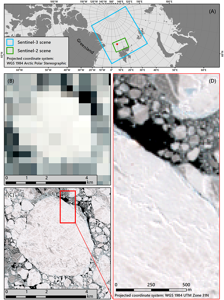
Figure 1. Comparison of Sentinel-2A (S-2A) and−3A (S-3A) spatial coverage and resolution [contains modified Copernicus Sentinel data (2017) processed by ESA/EOM]. (A) Coverage of S-3A/OLCI and S-2A/MSI scenes, the red dot indicates the location of (B). (B) Ice floe acquired with S-3A/OLCI (300 m, RGB: 665, 560, and 490 nm) at 2017-06-10 14:00:15 UTC. (C) The same floe acquired with S-2A (10 m, RGB: 665, 560, and 490 nm) at 2017-06-10 14:58:01 UTC. (D) S-2A details.

ESA's Sentinel-2 mission (S-2) offers new opportunities for optical sensors in the Landsat-like spatial domain. S-2 consists of the twin satellites S-2A and S-2B, launched in 2015 and 2017, respectively. Both satellites are equipped with the MultiSpectral Instrument (MSI), which provides 13 spectral bands with a 12-bit radiometric resolution in the wavelength region from 443 to 2,202 nm. Depending on the band, spatial resolution varies between 10, 20, and 60 m (European Space Agency, 2015, 2018a). Figure 2 illustrates the spatial and spectral settings of S-2A. Compared to L-7, S-2 has a larger swath width (290 km) and geographical coverage reaches up to 83° north. The two S-2 satellites are shifted by 180° on the same orbit, which results in a return period of 5 days. In higher latitudes, overlapping swaths further increase the return period to up to one image per day (European Space Agency, 2015, 2018b; Copernicus EO Support, personal communication). Due to the terrestrial focus of the S-2 mission, geographical coverage in the Arctic Ocean is currently limited to areas around islands but areas of interest may be added to the Mission baseline “if sufficient resources are identified” (European Space Agency, 2015). Malenovský et al. (2012) mentioned the potential of S-2 for albedo retrieval, derivation of snow properties and mapping of polynyas and leads; nevertheless, they also highlighted the demand for “precise corrections for atmospheric propagation, topography and directional reflectance behavior” (Malenovský et al., 2012), pointing to the importance of atmospheric correction (AC) of optical remote sensing data. Zege et al. (2015) also emphasized the importance of AC for the retrieval of melt pond fraction and surface albedo.

FIGURE 2

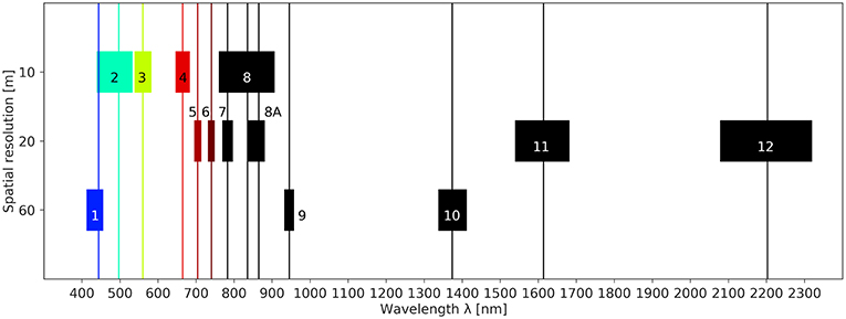
Figure 2. S-2A MSI band widths, central wavelengths and spatial resolutions.

Radiative transfer through the atmosphere is strongly influenced by Rayleigh and Mie scattering as well as aerosol and gas absorption. This combination is particularly challenging over water areas, where the atmospheric path radiance is typically >85% of the total signal in oceanic waters, >60% in sediment-rich waters, and >94% in very dark waters (IOCCG, 2010). Low sun-zenith angles (>70°) and correspondingly long atmospheric paths further aggravate the processing of data at the beginning and the end of summer in high latitudes (IOCCG, 2015). An adequate AC is therefore essential for the derivation of physical surface properties and follow-up multi-temporal analyses. Another challenge resulting from atmospheric transfer and the scattering of radiation is the neighboring or adjacency effect, i.e., the scattering of light from neighboring surfaces into the sensors field of view resulting in information overlay (Sterckx et al., 2015b). Adjacency effects depend on the brightness contrast between a target pixel and its neighborhood (Richter et al., 2006). The Arctic sea ice is a mix of snow, ice, melt ponds and ocean water, with typical broadband albedos in the visible wavelength region (VIS) ranging from >0.90 for fresh snow to <0.05–0.1 for ocean water (Perovich et al., 1998). Moreover, while being negligible for wavelength regions >1.5 μm, the adjacency effect increases with shorter wavelengths (Richter and Schläpfer, 2017), i.e., the wavelength region used for water remote sensing is heavily affected. Due to the characteristic spatial mixture and high contrasts of deep, clear ocean waters, melt ponds, bright ice and snow surfaces in the sea ice, we expect the adjacency effect to have a large impact on S-2 imagery of Arctic sea ice.

Several AC processors are available for S-2, and some papers already compared processors for lakes (e.g., Dörnhöfer et al., 2016; Martins et al., 2017). Only recently, Doxani et al. (2018) performed an inter-comparison of AC processors for different surface types in temperate and tropical zones. Yet, to our knowledge, no study exists for Arctic sea ice; therefore, the objective of this paper is to evaluate the performance of AC processors for S-2 over different surface types in the Arctic sea ice. For this, we processed S-2A data applying five AC processors (ACOLITE, ATCOR, iCOR, Polymer, and Sen2Cor) and evaluated the results using in situ data from open water and ice floe surface measurements acquired during an RV Polarstern cruise in June 2017. We further investigate the influence of different AC processors on the retrieval of apparent optical properties, i.e., surface reflectance and remote sensing reflectance, which are used to retrieve parameters such as the spectral albedo or NDMI.

Methods

Study Area

Cruise Overview

During cruise PS106.1 RV Polarstern was moored to an ice floe north of Svalbard between June 3 and 16, 2017 (Figure 3). At the beginning of the measurement period, snow and white ice covered most of the floe. Some few ponds had already formed at pressure ridges but we did not observe any pond formation on the flat parts of the floe; bare ice was exposed only very occasionally. Neither ponds nor bare ice were present near the measurement sites. Melting, however, started during the measurement period. The specific surface area of snow samples from the top 1–2 cm has been analyzed with an IceCube (A2 Photonic Sensors, France) at different locations in the area of interest. Snow melt results in a decrease of the snow's specific surface area. Figure 4 illustrates that melt occurred between June 4 and 10.

FIGURE 3

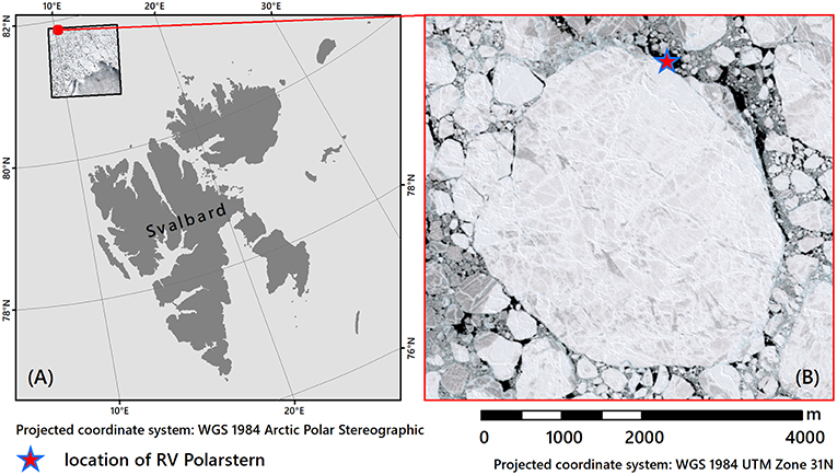
Figure 3. Location of S-2 granule (A) and ice floe (B) in the Arctic Ocean on June 10, 2017.

FIGURE 4

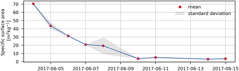
Figure 4. Specific surface area of snow at different locations between 2017-06-04 and 2017-06-15.

Atmospheric Parameters

To provide input data for the different AC processors, we used sun photometer measurements conducted on board of RV Polarstern and published in the Maritime Aerosol Network (AERONET-MAN, Holben et al., 1998). For later analysis, we computed the aerosol optical thickness (AOT) at 550 nm from the sun photometer measurements as:

$\begin{array}{rc}\beta =\frac{AO{T}_{\lambda }}{{(\lambda /550)}^{-\alpha }}& (1)\end{array}$

with β being turbidity, i.e., AOT at 550 nm, AOT_λ being the mean AOT at λ (500 nm) and α being the mean Angstrom exponent between 440 and 870 nm. We further used data from the weather station on board RV Polarstern (Schmithüsen, 2018). Table 1 summarizes minimum, maximum, mean and standard deviation of the atmospheric parameters used to atmospherically correct the S-2 data acquired on June 10, 2017 (details on S-2 data are provided in section Sentinel-2 Data).

TABLE 1

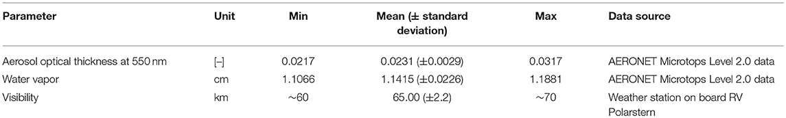
Table 1. Atmospheric parameters.

In Situ Data

To validate the results of the AC processors, we performed radiometric measurements of snow and ice covered areas (section Snow and Ice Measurements on the Floe) as well as open water (section Open-Water Measurements). Simultaneously to the radiometric open water measurements, we took water samples for water constituent analysis (section Water Sampling). All measurements have been localized with Global Positioning System (GPS) measurements (section Positioning of Sampling Points).

Radiometric Measurements

Snow and ice measurements on the floe

For spectral measurements on the floe, we used an ASD LabSpec5000 spectrometer (Analytical Spectral Devices Inc., United States), covering the wavelength region from 350 to 2,500 nm with a 1 nm spectral sampling rate. The ASD was equipped with an optical fiber with a 23° field of view (FOV) mounted to a pistol grip attached to a pole to avoid influences of the polar suits during the measurements (Figure 5A). We used a Labsphere Spectralon reflectance standard with 95% diffuse reflectance (Labsphere Inc., United States) as white reference. In addition, we used a set of Ocean Optics STS-VIS spectrometers (Ocean Optics Inc., United States). The setup consists of two synchronized spectrometers; one pointing downwards with a 1° FOV and the other, equipped with a diffusor, pointing upwards to track planar incoming radiation. Both instruments cover a wavelength region from 340 to 820 nm with a spectral sampling rate <1 nm. The spectrometers have also been attached to the end of a pole to avoid influences of the polar suits on the measurements (Figure 5B). For the Ocean Optics Instruments, we used a Labsphere Spectralon 99% diffuse reflectance standard (Labsphere Inc., United States) as white reference. For both instrument setups, we took reference measurements at intervals <10 min and when illumination conditions changed. Before conducting a white reference measurement with the ASD, we measured the Spectralon panel to control whether illumination has changed since the last reference measurement. If we detected changes, we performed a visual quality check on all measurements since the previous white reference and deleted spectra with unusual shapes. We corrected the Ocean Optics measurements for irradiance changes using the upwards pointing sensor. To account for the spatial heterogeneity within one S-2 pixel, we either walked around during the measurement process or performed measurements at different sites that we chose randomly. Table 2 summarizes measurement dates, instruments and illumination conditions.

FIGURE 5

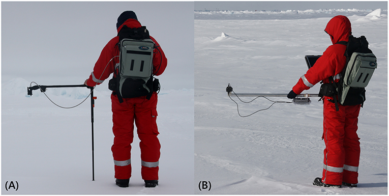
Figure 5. Measurement setups for ASD (A) and Ocean Optics (B) spectrometers. Photos: Natascha Oppelt.

TABLE 2

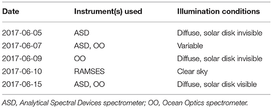
Table 2. Illumination conditions and instruments used.

Open-water measurements

In open-sea water of a polynya, we conducted radiometric measurements from the deck of the vessel using three hyperspectral (380–950 nm) RAMSES sensors (TriOS GmbH, Germany). The sensors were arranged to measure downwelling irradiance (E_d), upwelling radiance just above the water surface (L_u; sensor viewing angle of 40° with 90° azimuth angle to the sun), and corresponding sky radiance (L_sky). We calculated remote sensing reflectance, R_rs, according to the following equation:

$\begin{array}{rc}{R}_{rs}(40°,90°)=\frac{L_u(40°,90°)-\rho L_{sky}(40°,90°)}{E_d}& (2)\end{array}$

The sea surface reflectance factor, ρ, depends on the sun-viewing geometry and wind-dependent roughness of the surface. Wind was light to moderate, but the limited fetch reduced roughness (mean square slope of the waves) compared to open sea. We applied the usually recommended surface reflactance factor of Mobley (1999) to determine the mean reflectance, in this case ρ = 0.0272. Moreover, we applied four different surface reflectance factors between 0.0176 and 0.03 (Mobley, 2015; Hieronymi, 2016) to account for potential effects of reduced roughness and polarization. This methodical variability together with temporal changes of the single measurements were taken into account to determine the standard deviation of the in situ measurements.

We resampled all field spectra to S-2A bands using the spectral response functions and central wavelengths (European Space Agency, 2018a,c).

Water Sampling

We took water samples from the polynya simultaneously to the radiometric measurements. Water samples were filtrated and optically analyzed in the ship's laboratory. We determined the spectral absorption properties using a PSICAM (Röttgers and Doerffer, 2007), a QFT-ICAM (Röttgers et al., 2016), and a Liquid Waveguide Capillary Cell (World Precision Instruments, United States). During the S-2A acquisition on June 10, the −1.7°C cold seawater had a salinity of ~34 PSU. The particle concentration was very low, yielding a total particulate absorption coefficient at 440 nm, a_p(440) of approximately 0.013 m⁻¹. The colored dissolved organic matter (CDOM) absorption at 440 nm, a_cdom(440), was 0.038 m⁻¹. The spectral shape of the particulate absorption indicates only to the presence of organic phytoplankton particles and no sediments; there is no significant particulate and CDOM absorption in the near infrared (>700 nm). The chlorophyll-a concentration (Chl-a) from the photometric measurements was 0.19 (±0.1) mg m⁻³; additional measurements with an AlgaeTorch (bbe Moldaenke GmbH, Germany) yielded Chl between 0.2 and 0.3 mg m⁻³. These results confirm that the sampled water was very clear during the measurement period.

Positioning of Sampling Points

During the measurement period (Table 2) the ice floe drifted several tens of kilometers. To relocate all field measurements in a satellite image, we performed a drift-correction. Three stationary GPS devices constantly tracked floe movement in a 10-s interval. Additionally, we determined the locations of all sampling points with GPS measurements (F5521gw, Ericsson, Sweden; Galaxy S7, Samsung, South Korea; eTrex 10, Garmin, United States) in the World Geodetic System 1984 reference system. To locate all measurements from different dates and times in a single satellite image, we first applied a Savitzky-Golay filter to smooth the positioning data of each of the stationary GPS devices; then we used a second order polynomial to interpolate points in a 1-s interval. In this way, we could allocate every field measurement to three stationary GPS positions. Using this data, we computed the distances from every field measurement position to each of the three stationary GPS devices at the respective time of data acquisition (t_{in situ}). To find the measurement locations on the floe at the time of satellite overpass (t_satellite) we fit the distances to the three stationary GPS devices at t_satellite to the distances computed at t_{in situ} using the method of least squares. Finally, we performed a visual quality control.

Sentinel-2 Data

On June 10, 2017, clear sky conditions allowed acquisition of S-2A data of the floe at 14:58:01 UTC. For this study, we used the S-2 L1C top of atmosphere (TOA) reflectance product (processing baseline: 02.05; European Space Agency, 2015). For AC evaluation, we used S-2 bands which are in the spectral range of the field instruments, i.e. S-2A bands 2–7 (490–783 nm) for sea ice surfaces and bands 2–7 plus band 8A (490–865 nm) for the open water surface. All processors provide a 10 m output, except ATCOR. Which only offers a 20 m output. To provide spatially comparable results, we therefore downsampled 10 m output data to a spatial resolution of 20 m by 2 × 2 pixel block averaging.

Regions of Interest

In general, a point-by-pixel comparison is necessary for an accurate validation of remote sensing data via in situ measurements. With a steadily drifting floe, however, we are unable to assess precise accuracies of GPS measurements and trilateration; we therefore dismissed a point-based validation. Instead, we defined a region of interest (ROI) for each measurement Section by computing a circular buffer with a 20 m radius around all GPS points belonging to one measurement section. We defined all pixels intersecting the respective buffer area to be one ROI. Table 3 lists the respective number of pixels and field spectra as well as the measurement device used for each ROI.

TABLE 3

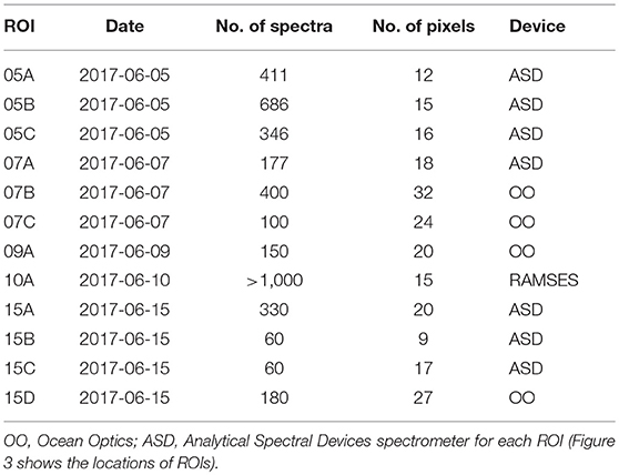
Table 3. Number of pixels, number of in situ spectra and measurement device.

Regarding the RAMSES measurements, we manually defined one ROI in the open water area next to RV Polarstern and excluded pixels with unusual shape presumably influenced by floating ice. Figure 6 illustrates locations of the respective ROIs.

FIGURE 6

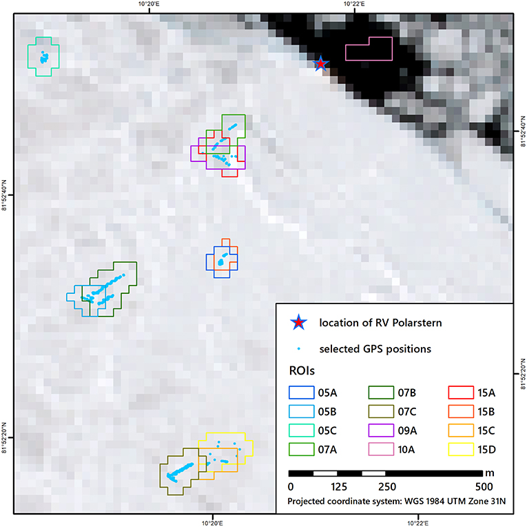
Figure 6. ROI locations on the investigated floe. Background: S-2A stretched pseudo-true color RGB image (RGB: 665, 560, and 490 nm, spatial resolution: 20 m) acquired at 2017-06-10 14:58:01 UTC.

Atmospheric Correction Processors

For our study, we selected common, publicly available AC algorithms. The level of user-controlled parametrization depends on the respective processor and is described in the following. Table 4 summarizes the most relevant parameters.

TABLE 4

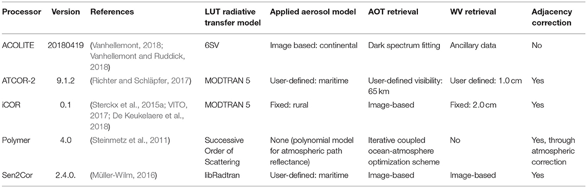
Table 4. Parametrization of AC processors used in this study.

ACOLITE is developed at the Royal Belgian Institute of Natural Sciences and includes AC processors specifically designed for aquatic applications, e.g., it addresses diffuse sky reflectance at the water surface. We used the most recent version that applies a new dark spectrum fitting AC by default (Vanhellemont, submitted). The algorithm consists of five steps (Vanhellemont and Ruddick, 2018): (1) Correction of atmospheric gas transmittance and sky reflectance in the TOA signal; (2) Construction of a dark spectrum using the darkest pixels in each band; (3) Estimation of AOT at 550 nm for different aerosol models (continental, maritime) by linearly interpolating path reflectance from look up tables (LUTs) generated with the Second Simulation of a Satellite Signal in the Solar Spectrum–Vector (6SV) radiative transfer model (Vermote et al., 1997); (4) Retaining the band resulting in the lowest AOT for each aerosol model; (5) AC with band and model combination resulting in overall lowest AOT. This approach is presumably more appropriate for ice surfaces than the black short-wave infrared approach of previous versions (Vanhellemont and Ruddick, 2015). Information on precipitable water, atmospheric pressure and ozone concentration are obtained from ancillary data. Adjacency effects are to some extent addressed in the aerosol correction procedure, but are not entirely extinguished (Vanhellemont and Ruddick, 2018). We used the default parameterization but changed the WV default value to 1.14 cm according to the AERONET data. The output of ACOLITE may be images of different reflectances such as surface reflectance or R_rs with a 10 m spatial resolution, which was downsampled afterwards.

ATCOR (Atmospheric/Topographic Correction for Satellite Imagery; Richter and Schläpfer, 2017) uses pre-calculated LUTs computed with the Moderate-Resolution Atmospheric Radiance and Transmittance Model–version 5 (MODTRAN 5) (Berk et al., 2008) and image-based retrievals of atmospheric properties. The LUTs cover four aerosol models (rural, urban, maritime, and desert) and six water vapor column contents (0.4–5.0 cm). Varying ozone concentrations are addressed via an extra ozone database. The dense dark vegetation method is used to derive AOT and the aerosol type can be estimated by comparison of derived path radiance with MODTRAN standard aerosol types. WV is estimated using the Atmospheric Pre-corrected Differential Absorption algorithm. The resulting unit is “bottom of atmosphere” (BOA) reflectance (Richter and Schläpfer, 2017). The interface of ATCOR guides the user through the parametrization of the processor, which enables to address emerging problems. The small number of dark pixels in the image hampered an image-based retrieval of aerosol type and AOT. A WV map could be generated, but values near the vessel were high (~1.8 cm) compared to the AERONET data. To parametrize the processor in accordance to the AERONET data, we therefore selected the pre-defined maritime aerosol type and a stable WV of 1.0 cm, which is the closest selectable default value, compared to the AERONET data. Visibility as a measure for AOT was set to 65 km. ATCOR considers adjacency effects as averaged reflectance of the neighborhood of a pixel (Richter and Schläpfer, 2017); its impact therefore depends on the difference in reflectance of a pixel and its neighborhood and decreases exponentially with increasing distance. Thus, for recurrent spatial patterns, adjacency effects remain similar at different spatial scales; consequently, the absolute range of the adjacency correction is uncritical. Therefore, we selected a typical range of 1 km (Richter and Schläpfer, 2017). The number of adjacency zones remained unchanged (1). We further applied a cirrus correction and selected the 20 m spatial resolution output.

In this study, we also used iCOR version 0.1 in ESA's Sentinel Application Platform (SNAP; v5.0). iCOR, previously known as OPERA (Sterckx et al., 2015a), is an AC processor for land and water as it accounts for the non-Lambertian reflectance of water surfaces. The iCOR workflow comprises four steps (De Keukelaere et al., 2018): (1) Classification of land/water pixels; (2) AOT retrieval over land following the approach in Guanter (2006), and extension to adjacent water pixels assuming a spatially homogeneous atmosphere; (3) adjacency correction; (4) AC using pre-calculated MODTRAN 5 LUTs based on a rural aerosol model (De Keukelaere et al., 2018). In the current iCOR SNAP version, WV is fixed to 2.0 cm. Over water the adjacency effect is corrected using the SIMilarity Environment Correction (SIMEC) approach (Sterckx et al., 2015b) while over land the user defines a fixed range (Sterckx et al., 2015a; VITO, 2017). We applied the adjacency correction and increased the default adjacency window for land surfaces to three pixels (tests with larger values introduced a reflectance peak at 705 nm). Further, we adjusted the default AOT value to 0.02 according to the AERONET data. Besides that, we used the default parameter setting. iCOR returns BOA reflectances in the native resolution of the respective band.

The polynomial-based atmospheric correction algorithm Polymer (Hygeos France; Steinmetz et al., 2011) is an AC processor for water bodies applicable to multiple sensors, including MSI and OLCI. Polymer is a spectral matching algorithm, which decouples the reflectance signal of the water body from atmospheric and water surface reflectance. It makes use of the observation that the sum of atmospheric path reflectance and adjacency effects can be approximated by a polynomial consisting of three terms that address (1) non-spectral scattering or reflection, (2) fine aerosol scattering and (3) molecular scattering and adjacency effects, and does not require an aerosol model (IOCCG, 2015). One of the strengths of Polymer is the possibility to retrieve R_rs in presence of sun glint, which leads to a higher yield of evaluable pixels compared to other algorithms. Recently, the Polymer algorithm has been modified to improve results in high latitudes (Steinmetz and Ramon, 2018). In the processing chain, non-water surfaces are masked, i.e., Polymer has only been applied to ROI 10A. For this study, the Polymer 10 m outputs were projected and resampled to the Sentinel-2 grid using the Nearest Neighbor approach, and spatially downsampled to 20 m resolution by 2 × 2 pixel block averaging.

Sen2Cor is the Sentinel-2 Level-2A Prototype processor for land surfaces. For this paper, we used the stand-alone version of Sen2Cor 2.4.0, which also allows for an image-based retrieval of atmospheric parameters. Water vapor is derived with the Atmospheric Pre-corrected Differential Absorption algorithm applied to S-2 bands 8A and 9. Sen2Cor estimates AOT by means of the dense dark vegetation method using the relation of the reflectance in bands 4, 2, and 12. The image-derived atmospheric parameters are then associated with pre-computed LUTs generated by a libRadtran based radiative transfer model. The LUTs include two atmospheric models (mid-latitude summer and winter), two aerosol types (maritime, rural), six or four different WV column values and six ozone concentrations (Müller-Wilm, 2016). We chose the maritime aerosol type and selected the mid-latitude winter model atmosphere as suggested in Harris Geospatial Solutions Inc (2018). We activated the variable visibility option and changed the default value to 65 km.

Performance Measures

We performed the spectral measurements on the floe within 5 days before and after the satellite acquisition. Illumination conditions therefore differed for field measurements and the satellite observation (see section Radiometric Measurements) which may affect measurement results (Malinka et al., 2016). Moreover, due to the different spectrometer setups described in section Snow and Ice Measurements on the Floe, ASD and Ocean Optics show varying sensitivities to changing illumination conditions. The different FOVs result in varying sensitivities to changing sensor-surface geometries. An inter-comparison of ASD and Ocean Optics under field conditions revealed mean differences in surface reflectance of about 0.1; a comparison of in situ spectra and BOA reflectances by means of classic performance metrics such as bias or root mean squared error therefore is unreasonable.

To identify systematic differences between the respective processors, i.e., the average tendency of the BOA reflectance to be larger or smaller than TOA reflectance, we computed the percentage bias (PBIAS) as

$PBIAS=100·\frac{{\displaystyle {\sum }_{i=1}^n\left(R^{AC}({\lambda }_i)-R^{TOA}({\lambda }_i)\right)}}{{\displaystyle {\sum }_{i=1}^n\left(R^{TOA}({\lambda }_i)\right)}}(3)$

with R^AC and R^TOA being the bottom and top of atmosphere reflectance at band λ_i, respectively; n is the number of bands.

Compared to the absolute values, spectral shapes are more stable, especially at the beginning of the melt season and for the visible wavelength regions (Perovich, 1994). We therefore evaluated the spectral shapes of ice and snow measurements on the floe, computing the slope between two adjacent bands and then calculate the slopes' Mean Absolute Error (slope MAE):

$\begin{array}{rc}slopeMAE=\frac{1}{n}{\displaystyle \sum _{i=1}^n}|S^{AC}({\lambda }_i,{\lambda }_{i+1})-S^{insitu}({\lambda }_i,{\lambda }_{i+1})|& (4)\end{array}$

with $S^{AC}({\lambda }_i,{\lambda }_{i+1})$ being the slope of the BOA reflectance outputs of the respective AC processor and $S^{insitu}({\lambda }_i,{\lambda }_{i+1})$ being the slope of the resampled in situ reflectance between band λ_i and band λ_i+1, respectively; n is the number of band pairs. We further calculated the coefficient of determination (r²) as the square of Pearson's correlation coefficient to evaluate linear correlations between the respective AC BOA output and the in situ measurement:

$\begin{array}{ll}{r}^2={\left(\frac{{\displaystyle {\sum }_{i=1}^n}\left(R^{insitu}\left({\lambda }_i\right)-\overline{R^{insitu}}\right)·\left(R^{AC}\left({\lambda }_i\right)-\overline{R^{AC}}\right)}{\sqrt{{\displaystyle {\sum }_{i=1}^n}{\left(R^{insitu}\left({\lambda }_i\right)-\overline{R^{insitu}}\right)}^2}·\sqrt{{\displaystyle {\sum }_{i=1}^n}{\left(R^{AC}\left({\lambda }_i\right)-\overline{R^{AC}}\right)}^2}}\right)}^2& (5)\end{array}$

with R^AC being the output of the respective AC processor and R^{in situ} being the reflectance of the resampled in situ spectrum at band λ_i (band 2–7); n is the number of bands.

For deep polynya water, we performed measurements of R_rs from the deck of the vessel parallel to the satellite overpass under clear-sky conditions. No white referencing was necessary due to the measurement setup, which already integrates changes in illumination conditions. We therefore compared resulting reflectance intensities. ACOLITE calculates R_rs, while ATCOR, iCOR, SEN2COR and Polymer yield surface reflectances. The surface reflectances were transformed into R_rs following (Mobley et al., 2018):

$\begin{array}{rc}{R}_{rs}=\frac{R^{AC}}{\pi }& (6)\end{array}$

with R^AC being the surface reflectance output of the respective AC processor. We then computed MAE to account for differences in reflectance intensity according to:

$\begin{array}{rc}MAE=\frac{1}{n}{\displaystyle \sum _{i=1}^n}|R_{rs}^{AC}({\lambda }_i)-R_{rs}^{insitu}({\lambda }_i)|& (7)\end{array}$

with $R_{rs}^{AC}$being Rrs of the respective AC processor and $R_{rs}^{insitu}$ being Rrs of the resampled in situ spectrum at band λ_i (band 2–8A); n is the number of bands. To evaluate correspondence in spectral shapes, we computed slope MAE and r², replacing surface reflectance with Rrs and expanding S-2A band selection by band 8A.

Results

Due to the different measurement designs described above, we discuss the results for open water as well as snow and ice surfaces separately.

Snow and Ice Surfaces

Figures 7A,C,E illustrates the mean shape and intensity of S2-A TOA reflectances, BOA reflectances of the respective AC processors and resampled in situ spectra from snow and ice surfaces. Due to the low variance, we computed the mean spectra of all ROIs on the floe. In situ spectra show the typical shapes of snow and ice with maximum reflectances in the blue-green wavelength region and a decrease toward longer wavelengths. Maximum mean in situ reflectances at band 2 (490 nm) range from approximately 0.8–1.1 with high standard deviations presumably resulting from a high spatial variability on sub-pixel scale. Values are in line with field measurements from other studies (e.g., Perovich, 1998; Goyens et al., 2018). In comparison to the TOA spectrum, BOA spectra for all AC processors show increased reflectances over the entire spectrum. For each ROI, Sen2Cor produces the highest BOA reflectances, also indicated by high PBIAS values (Table 5). On average, Sen2Cor BOA reflectances are about 30 % higher than TOA reflectances. BOA reflectances of iCOR (mean PBIAS: 10.8%) and ATCOR (mean PBIAS: 11.7%) are generally lower than Sen2Cor values and resemble each other in intensity and shape. Yet, in comparison to iCOR, ATCOR BOA reflectances decrease slightly with shorter wavelengths. ACOLITE BOA reflectances are lowest for all ROIs and only 6.6% higher than TOA reflectances, on average. Figure 7E illustrates the slopes of the respective spectra showing largest differences for Sen2Cor (mean slope MAE: 1.17E-03); high slope MAE values in Table 5 confirm this observation. For iCOR (mean slope MAE: 2.64E-04) and ATCOR (mean slope MAE: 2.29E-04), Figure 7E highlights differences in bands 2–4 and similarities in bands 5–7. Overall, ACOLITE fits the shape of the resampled in situ spectrum best, also indicated by low slope MAE values in Table 5 (mean slope MAE: 1.92E-04). Coefficients of determination in Table 5 confirm this trend and are highest for ACOLITE (mean r²: 0.9758), followed by ATCOR (mean r²: 0.9728) and iCOR (mean r²: 0.9702), while Sen2Cor shows the weakest linear relationship (mean r²: 0.9137), on average.

FIGURE 7

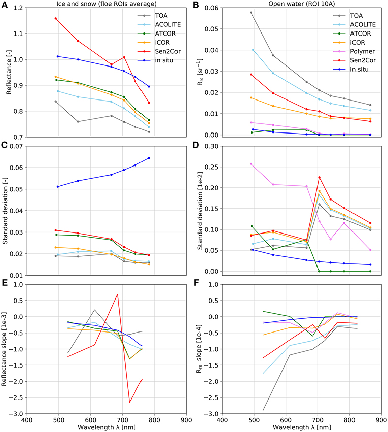
Figure 7. Mean resampled in situ spectrum, S-2A TOA spectrum and BOA outputs of different AC processors for ice and snow ROIs (A), respective standard deviations (C) and spectral slopes (E). Mean resampled in situ spectrum, S-2A TOA and BOA R_rs outputs of different AC processors for the open water ROI 10A (B), respective standard deviations (D) and spectral slopes (F).

TABLE 5

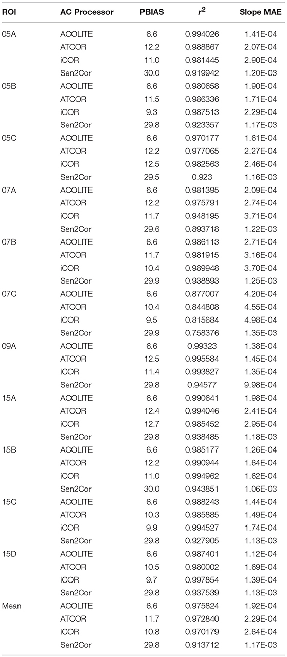
Table 5. Performance measures of resampled mean in situ and BOA spectra for different ROIs on the ice floe.

Open Water

Figures 7B,D,F illustrates the results for the open water measurements. It is obvious that ACOLITE and Sen2Cor intensities are one order of magnitude higher than the in situ values, also demonstrated by high MAE values in Table 6. High coefficients of determination (r²~0.96), however, indicate a strong linear correlation between resampled in situ and R_rs spectra, although the spectral slope is different (slope MAE in Table 6 and Figure 7). iCOR average R_rs is almost 10 times higher than average in situ data (MAE~0.01), but spectral shape is more similar compared to ACOLITE and Sen2Cor indicated by a small slope MAE (2.17E-05) and high r² (~0.97). Polymer retrieved R_rs are in the same order of magnitude as measured R_rs, illustrated by a small MAE of 0.0015, while ACOLITE, iCOR and Sen2Cor overestimate R_rs. The lowest slope MAE (1.54E-05) indicates that Polymer resembles the shape of the in situ spectrum most accurately. The comparably weak correlation (r²~0.85) results from a drop of the spectrum in bands 5–8A (Figure 7B). The ATCOR output is also in the correct order of magnitude over the full spectrum and has the smallest MAE and a comparable low slope MAE. It has to be noted, however, that the spectral shape in the visible range differs, also indicated by a weak linear correlation (r²~0.18). The slope MAE is higher than for Polymer, highlighting the difference in shape in visible bands 2 (490 nm) to 4 (665 nm).

TABLE 6

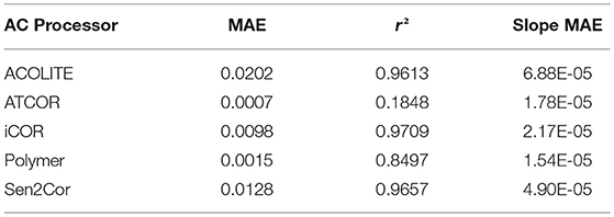
Table 6. Performance measures of resampled mean in situ and R_rs spectra for respective AC processors in comparison with mean resampled in situ spectrum at ROI 10A.

Application Examples

To illustrate the consequences of different ACs on parameter retrieval, we computed the average BOA reflectance from band 2 to 7 (490–782 nm) as a rough approximation to broadband albedo (Figure 8). In addition, we calculated NDMI, which can be used as a proxy for melt pond fraction (Istomina and Heygster, 2017) according to

$\begin{array}{rc}NDMI=\frac{{\lambda }_{Green}-{\lambda }_{NIR}}{{\lambda }_{Green}+{\lambda }_{NIR}}& (8)\end{array}$

where λ_Green is S-2 band 3 (560 nm) and λ_NIR is S-2 band 8A (865 nm) from the respective AC product. Theoretically, NDMI values range from −1 to +1. Due to the specific reflectance characteristics of the different sea ice surfaces in these wavelength regions the value range, however, is practically limited to values >0. Increasing values indicate an increasing melt pond fraction. Figure 8 illustrates that the AC processor influences parameter retrieval and, in reverse, that the application rules the choice of AC processor. Note that median TOA reflectance of the floe surface is 0.75, and BOA reflectances are approximately 0.80 in the ACOLITE product and ~0.84 in the ATCOR and iCOR products, reaching 0.97 in the Sen2Cor product. In general, NDMI results show the same pattern, whereas median NDMI values are lowest for TOA (0.06), followed by ACOLITE (0.12), ATCOR (0.13), iCOR (0.14), and Sen2Cor (0.18). This corresponds to the spectral behavior illustrated in Figure 7.

FIGURE 8

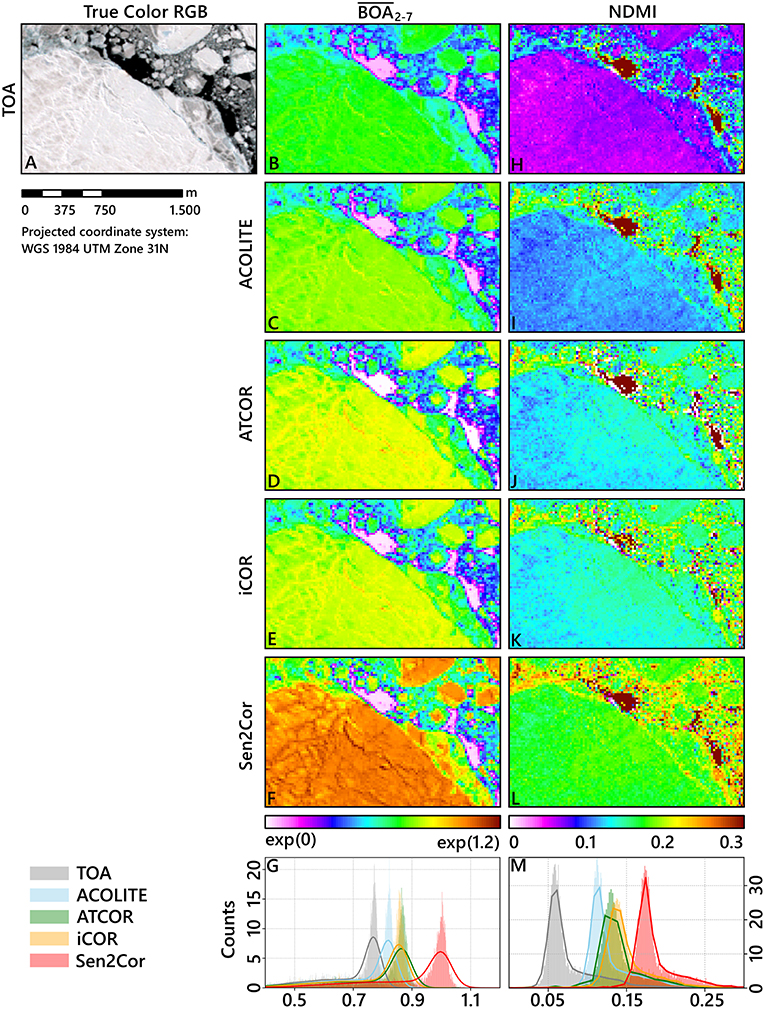
Figure 8. True color RGB image (A); band 2–7 average of TOA (B) and BOA (C–F); NDMI results for TOA (H) and BOA (I–L); and histograms of the respective parameters for the image subset (G,M).

Discussion

Comparability of Field and Satellite Data

The comparison of field spectroscopy and satellite observations involves a number of difficulties, which particularly applies to remote regions such as the Arctic where ideal measurement opportunities and coincident satellite overpasses are rare. We conducted spectral measurements of the floe surface within a period of ±5 days of the satellite overpass under varying illumination conditions and possibly changing surface properties due to the onset of melt. We postulate, however, that an analysis of spectral shapes is reasonable as the anisotropic reflectance factor of snow at nadir is ~1 (Perovich, 1994) and the shape of the spectral albedo is constant under different illumination angles (Malinka et al., 2016). For snow surfaces, Goyens et al. (2018) and Bourgeois et al. (2006) observed no significant relationship between variations in reflectance anisotropy with illumination conditions for sun zenith angles <65°. In addition, the effect of melt on the spectral shape of nadir reflectance of snow and ice is comparably low in the VIS (Perovich, 1994, 1998). Nevertheless, we are unable to exclude potential differences in spectral slope due to melt processes. Besides the temporal differences, it is challenging to represent the spatial variability within a 20 m × 20 m area measured by S2-A via field measurements, even when measured at different locations. Moreover, a re-location of the measurement positions on a drifting floe in combination with spatial uncertainties of both GPS devices and satellite image positioning exacerbates a point-by-pixel comparison. For this reason, we included surrounding pixels into the analysis. However, this method is vulnerable to extreme spectral features in a ROI that can have a great impact on the average spectrum. The standard deviations of the ROIs located on the floe, however, are small indicating low spectral variability (Figure 7C); we therefore assume the ROI approach to be a valid method for evaluating the AC processors. ROI 10A over open water was defined manually and excluded pixel with unusual shape, presumably resulting from sub-pixel contamination due to floating ice. This pre-selection may substantially influence the outcome of the study, as pixel with expected shape are preselected. The pre-selection, however, avoids integration of extreme spectral features, which may have a major influence on the average spectrum due to sub-pixel contamination.

Quality of In Situ Data

For some ROIs, field spectrometer data show reflectances >1.0, although both field spectrometer setups were calibrated with reflectance standards. The Ocean Optics setup also enabled the correction of illumination changes. For ASD measurements, we surveyed changes in illumination by measuring the reflectance standards before each subsequent calibration. We manually deleted ASD measurements affected by illumination changes, i.e., spectra with unusual shape. Successive spectra with stable shape showing reflectances >1.0, however, remained in the dataset. In addition to the differences regarding sensitivity to changes in illumination, both setups vary regarding their FOVs. The smaller FOV of the Ocean Optics makes it more vulnerable to twisting of the pole and anisotropic effects due to ice surface topography. An inter-comparison of spectrometers in the field revealed that Ocean Optics reflectance values are ~0.1 higher than ASD reflectances, on average, while the spectral shape was very similar. Warren (1982) stated that cloud cover affects both the spectral distribution of irradiance and the effective incident zenith angle, which causes an increase in all-wave snow albedo of up to 11%. Painter and Dozier (2004) attributed reflectances >1.0 to anisotropic effects of snow, which depend on the sun zenith angle, the grain size and the viewing geometry. Anisotropic effects may also have influenced the measurements described by Goyens et al. (2018) and Perovich (1998), who report reflectances >1.0 at approximately 400 nm measured under clear sky conditions. Peltoniemi et al. (2005) included snow wetness as an additional parameter influencing the spectral albedo and anisotropic behavior of snow and ice surfaces. As we evaluate the spectra only regarding to their shape, however, results remain unaffected by values >1.0. Analysis of water samples in the deep-water polynia show no significant absorption or scattering of the water constituents in the near infrared spectral range (>700 nm). Accordingly, beyond the visible range, measured R_rs is smaller than 1.5 × 10⁻⁴, i.e., near zero (black) in the near infrared. Measurements influenced by ice floating into the FOV of the RAMSES spectrometer were excluded from the evaluation. The AERONET AOT values (~0.02) are within the range reported for typical Arctic background aerosol concentrations, with values between 0.02 and 0.08 (Tomasi et al., 2012; IOCCG, 2015).

AC Processors

Differences between BOA or R_rs products may originate from the different processors, the integrated LUTs, different parameterization and image-based parameter retrieval regarding WV content, aerosol type and AOT, or different adjacency correction schemes, and the interplay of these components. Varying options for the user to modify the parameterization further complicate a direct comparison. Moreover, some of the processors are still under development and not yet entirely documented which hinders a detailed reasoning.

The LUTs applied in the AC processors have been generated with different radiative transfer models (MODTRAN 5, 6SV, libRadtran, and Successive Order of Scattering). These models differ regarding the implementation of physical equations, approximation of the radiative transfer equation and subroutines which can result in differences (e.g., Callieco and Dell'Acqua, 2011). Evaluating the impact of a certain radiative transfer model on AC, however, is beyond the scope of this study. The aerosol models covered by the pre-calculated LUTs cover common aerosol types. The options, however, differ between the AC processors (section Atmospheric Correction Processors). It is questionable how well these models represent Arctic aerosol components, e.g., mineral dust, sulfate aerosols and sea salt (at Barrow, Alaska; Tomasi et al., 2012; IOCCG, 2015). In late spring and summer, a phenomenon known as Arctic Haze results from anthropogenic aerosol accumulation in winter is common and occasionally aerosols from forest fires or volcanic eruptions are observed (IOCCG, 2015). To analyze the impact of the aerosol model we conducted a sensitivity analysis with different aerosol models in ATCOR. For the desert, maritime and rural aerosol models, differences in the VIS bands for the bright snow and ice surfaces were ~2%, while the urban aerosol model resulted in an increase of ~5–10% reflectance.

ACOLITE is designed for aquatic applications; the main differences compared to other AC processors are the AOT retrieval by the dark spectrum fitting algorithm and the consideration of skyglint. Its performance over ice surfaces, however, is good regarding the shape of BOA reflectance spectra. For sea ice surfaces differences in surface reflectance due to skyglint correction are <0.02. No water vapor and ozone values could be obtained from ancillary data, which might due to the developmental state of the processor; thus, the default values were used for AC and it remains unclear if the retrieval of water vapor and ozone in the Arctic from ancillary data is possible. Given the applied parameterization, the dark spectrum fitting algorithm results in the application of a continental aerosol model and an AOT of 0.0084 at 550 nm, i.e., comparably close to the measured value of 0.02 (AERONET-MAN reports uncertainties ≤0.02 per band; NASA Goddard Space Flight Center, 2017). We assume that the high R_rs values over water result from adjacency effects, which are not addressed by ACOLITE.

ATCOR performs well over ice surfaces while its performance over open water is poor as the spectral shapes of BOA and in situ data do not correspond. Due to the lack of dark pixels in the S2-A data set we defined AOT by visibility (65 km), illustrating that the dark vegetation method is unsuitable for AOT retrieval in this image. For WV, image-based retrieval resulted in an overestimation of WV (~1.8 cm). We therefore defined a default value (1.0 cm) referring to the AERONET data. Few pixels (1.2–1.4%) of bands 5–9 show negative reflectance values at open water areas, which may be caused by underestimated visibility, the aerosol type or calibration issues. Application of haze removal was not possible due to the small amount of clear pixels (<4%). Increasing the visibility parameter (up to 120 km) only had negligible consequences for the snow and ice surfaces and did not improve the spectral shape of open water pixels. This corresponds to Huck et al. (2007) who found that increasing visibility in a 6S forward simulation for AVHRR only affects open water surfaces. Changing the WV content from 1.8 to 1.0 cm had a significant influence, especially in S-2 bands that cover WV absorption features, i.e., band 8 (842 nm), band 9 (940 nm), and also band 5 (705 nm). For simulated Sea-viewing Wide Field-of-view Sensor (SeaWiFS) like spectra at the edge between sea ice and open water, Bélanger et al. (2007) found contaminations due to the adjacency effect up to 24 km off the ice edge resulting in unreliable results in derived chlorophyll concentrations and optical properties of open ocean water. Bulgarelli and Zibordi (2018) found that for S-2/MSI adjacency effects caused by highly reflecting surfaces (e.g., snow) are theoretically detectable at least 20 km off the coast in mid-latitude coastal environments. In contrast to these simulations, the area of interest is characterized by a small-scale mixture of snow, ice, melt ponds and open water, where spatial patterns and average reflectance are similar on different spatial scales. To check whether this statement applies for sea ice, we tested different ranges (1, 3, 5, and 10 km) and results confirmed that the influence is negligible for the spectral shape of the snow surface and intensity of open water pixels.

iCOR addresses the requirements for aquatic and terrestrial surfaces including a correction of adjacency effects. iCOR was unable to assess AOT from the image as the retrieval algorithm relies on vegetation and soil pixels (De Keukelaere et al., 2018), questioning the suitability of this approach for the Arctic sea ice in the absence of in situ AOT values. Even though, the fixed WV column height of 2.0 cm showed good results over ice, iCOR's unknown sensitivity to WV aggravates AC processor inter-comparison. The good performance over water compared to ACOLITE and Sen2Cor is probably attributed to the correction of adjacency effects using the SIMEC algorithm. For the application of SIMEC, Sterckx et al. (2015b) point out that aerosol information (AOT and aerosol model) should be either estimated using a land-based aerosol retrieval or from sun photometer data. While we used AERONET data to set the default AOT, we could not parameterize the aerosol type. Further, SIMEC is based on the assumption that reflectance differences between water and surrounding surfaces are strongest in the NIR, which is true for vegetated surfaces but not for ice, where differences are strongest in the VIS. We found that iCOR is very sensitive to changes in AOT. Increasing AOT from 0.02 to 0.1 resulted in an overcorrection and, consequently, a decrease of the spectrum matching the in situ measurements very well (slope MAE ~8.49E-06).

Polymer performs best over water and produces reasonable results even in the high contrast Arctic sea ice matching findings of Steinmetz and Ramon (2018). It is robust to adjacency effects because the atmospheric model fits any spectrally smooth non-water component (Steinmetz and Ramon, 2018). The manual definition of ROI 10A guaranteed that we only considered deep-water pixels, which may also be important for the good performance of Polymer. Nevertheless, we observe a high spectral variability in the VIS bands. Moreover, some negative values appear in the red-edge and NIR regions. Sub-pixel contamination due to floating ice should be corrected due to its spectrally-flat contribution to the reflectance signal.

Usually, Sen2Cor applies image-based retrievals to generate maps of AOT and WV. The lack of dark pixels in the S-2A image, however, prohibited an AOT retrieval based on the DDV method; thus, AOT was estimated from the provided visibility (65 km). Values for scene average WV and AOT at 550 nm are 1.51 cm and 0.132, respectively. Compared to the AERONET data, however, both values are very high. A further test with a fixed visibility of 120 km, corresponding to an AOT of ~0.0780, as proposed by Pflug et al. (2016) as a good practice for clear air and low AOT over Antarctica, did not improve the results for BOA reflectance and R_rs significantly. The increased BOA reflectance in comparison to the other processors fit findings of Li et al. (2018) who report that surface reflectance derived with Sen2Cor is generally overestimated, in particular for bright pixels. The high values over water may be attributed to the lacking correction of skyglint and adjacency effects or the provided LUTs.

A general challenge in high latitudes is the low sun elevation throughout long periods of the year. Huck et al. (2007) found that the solar zenith angle has a major influence on the retrieved TOA reflectance of a nadir-viewing sensor. The low reflectance levels of water bodies further increase this effect, because atmospheric path length increases with decreasing sun elevation. Consequently, the amount of energy absorbed in the atmosphere increases while the amount that arrives at the Earth's surface decreases. At the same time, the amount of light that is specularly reflected at the water surface increases with decreasing sun elevation, while a lower amount is transmitted into the water body. As a consequence, the water body scatters less light toward the sensor (Hieronymi, 2013). Further, the influence of surface roughness on the transmission of light into the waterbody increases with sun zenith angle which challenge wind speed-dependent AC (Hieronymi, 2016). When the sun is close to the horizon, adjacent ice floes may also have a shading effect. The same applies for ice floes, where shadows of ridges increase with lower sun elevation and anisotropic effects increase for sun-zenith angles >65° (Bourgeois et al., 2006). Another issue regarding low sun elevation is the limitation of most processors to sun zenith angles ≤70°. The reason is that the LUTs are generated with radiative transfer models that base on the assumption of a plane parallel atmosphere rather than an actual spherical-shell atmosphere (IOCCG, 2015). Since in our study the sun zenith angle is 62.5°, we assume that this effect is negligible.

Sentinel-2A Data

Typically, reflectance spectra of snow and ice (like in situ spectra) are characterized by a steady decrease from the blue domain toward longer wavelength regions. S-2A TOA spectra, however, show a steep decrease from band 2 to 3 (490 and 560 nm, respectively), followed by an increase from band 3 to 4 (560–665 nm; Figure 7A). A comparison of BOA reflectance spectra with typical spectra found in literature (e.g., Perovich, 1994, 1998) indicates that ACOLITE, ATCOR and iCOR produce realistic results. As described in section Comparability of Field and Satellite Data, however, melt processes may have caused reflectance changes between in situ and satellite data. Thus, the evaluation of BOA spectral shape is challenging. In general, however, BOA shapes of ACOLITE, ATCOR, and iCOR are similar to the shape of the in situ spectra, i.e., the differences in slope MAE and r² are small. The shapes of Sen2Cor BOA reflectances do not resemble the typical shapes of snow and ice spectra as they show a steep decrease from the blue wavelength region toward longer wavelengths, interrupted by a local peak in band 5 at 705 nm. Furthermore, Sen2Cor is the only processor that produces reflectance values >1.0. Nadir reflectances of snow and white ice may exceed 1.0 in the blue part of the electromagnetic spectrum (e.g., Perovich, 1994; Goyens et al., 2018) but Sen2Cor BOA reflectances exceed 1.0 even in bands 3 and 4 (560 and 665 nm, respectively). This may result from anisotropic effects due to snow parameters or floe topography and matches observations of Li et al. (2018) who found that Sen2Cor overestimates BOA reflectance; ACOLITE, ATCOR, and iCOR BOA reflectance values, however, are <1.0 in all bands.

Application Examples

As indicated in section Application Examples, the choice of AC processor influences parameter retrieval. The differences in BOA reflectance illustrated in Figure 7 have a great impact on NDMI and surface albedo (Figure 8), which is roughly approximated here by the mean BOA reflectance of bands 2–7 (490–783 nm). The shifted peaks in the histograms refer to the offset-like behavior of the spectra from different AC processors illustrated in Figure 7. The example illustrates well that the application of a certain AC processor and resulting BOA reflectances affects the retrieval of geophysical parameters from S-2A imagery.

Conclusion

ESA's S-2 mission shows high potential to assist sea ice research. The high spatial resolution allows detailed observation of small-scale sea ice features such as ridges and melt ponds. Thus, S-2 can be used to bridge the spatial scale between in situ observations and very high spatial resolution imagery, e.g., from airborne sensors, to coarse resolution sensors such as Sentinel-3. Even though geographical coverage in the Arctic Ocean is currently limited to areas close to the shore, coverage may be extended on request (European Space Agency, 2015). The temporal scale may be bridged either by comparison of identical granules from multiple dates or by multiple images of the same floe. For all subsequent applications such as change detection and time series analysis, however, AC is a crucial step in the processing chain of S-2 data as it is a requirement for an accurate retrieval of geophysical parameters.

We applied five AC processors for S-2 (i.e., ACOLITE, ATCOR, iCOR, Polymer, and Sen2Cor) to a S-2A dataset acquired north of Svalbard on June 10, 2017 and analyzed the results for snow and ice surfaces as well as for deep-water areas. For this dataset, the ACOLITE dark spectrum fitting algorithm resembled the shape of the mean resampled in situ spectra of the floe surface in the wavelength region 490–783 nm most accurately, closely followed by ATCOR and iCOR. Considering potential influences of melt on the spectral slope, a conclusive assessment, however, is challenging as ACOLITE, ATCOR and iCOR resembled the typical shape of snow reflectance. Results of this study, however, indicate that the present version of Sen2Cor is unsuitable for applications in the Arctic sea ice.

Due to the field measurement setup, our study was incapable of evaluating AC quality in terms of absolute intensities. Hence, future validation measurements on sea ice are necessary. Field measurements of the water surface concurrent to the S-2A overpass allowed a direct comparison of in situ data and AC products. Coefficients of determination indicate a strong linear relationship between the mean resampled in situ spectrum and ACOLITE, iCOR, and Sen2Cor BOA reflectances, respectively; their spectral slope, however, differs and intensities are one order of magnitude higher. Regarding absolute intensities and slope MAE, Polymer produced the best results, while ATCOR performed poorly over open-water areas. At the time of the S-2A overpass, existing ponds were too small to be included in this study. Future investigations should therefore also address the applicability of AC processors on optically shallow melt pond water.

We further demonstrated the influence of different AC processors on the retrieval of geophysical parameters. Depending on the processor, medians of average reflectances and NDMI for an image subset range from 0.80 to 0.97, and 0.12 to 0.18, respectively. Medians of average reflectance and NDMI are 0.75 and 0.06, respectively. We expect the impact on models that rely on absolute intensities instead of ratios to be even higher. In our study, the retrieval of AOT was critical. The absence of surface types such as dense dark vegetation (which are relevant for image-based retrieval of atmospheric parameters such as AOT) turned out as a general issue for all processors. ATCOR, Sen2Cor, and iCOR failed to retrieve aerosol information from the image, AOT estimated by the new ACOLITE dark spectrum fitting algorithm, however, was in the margin of uncertainty of the AERONET data. Sensitivity analyses with ATCOR and Sen2Cor, however, indicate that AOT, i.e., visibility, is not a limiting factor regarding bright ice surface BOA reflectance. Apparently, the influence of AOT on the spectral shape is negligible if some threshold (≤65 km) is exceeded. Image-based retrieval of WV by ATCOR and Sen2Cor and sun photometer data also discorded. With lacking sun photometer data, information about total columnar WV and ozone for processor parameterization, we therefore recommend using predefined aerosol models over ice; nevertheless, we strongly underline the need for image-based retrievals for scenes only containing Arctic sea ice. We further encourage the implementation of an Arctic Background aerosol model (Tomasi et al., 2007) as done by Zege et al. (2015) into existing processors. Until then, the integration of ancillary data might improve BOA retrieval. Yet, further tests are necessary to estimate the quality and availability of ancillary data in the Arctic.

Our study showed that AOT has a large impact on optically deep water. Since Polymer is independent from AOT and aerosol type estimation and insensitive to adjacency effects, it shows a huge potential for the Arctic Ocean. Further field studies, however, should be carried out to explore its capabilities, e.g., for the detection of algae blooms; and extrapolation of the atmospheric signal to adjacent ice floes may also enable AC of ice and snow surfaces. Similarly to Bélanger et al. (2007) and Huck et al. (2007), a sensitivity analysis based on forward modeling of atmospheric transfer to generate S-2A like TOA signals from in situ measurements may also support the improvement of existing processors.

Data Availability

Reflectance measurements, positions and regions of interest are available at the PANGAEA data repository under doi.pangaea.de/10.1594/PANGAEA.898552.

Author Contributions

MK, MH, and NO conceived and designed the study. MK wrote the paper and conducted image and data processing and analysis. MH processed RAMSES data, analyzed water samples and contributed the respective passages. All authors contributed equally in reviewing and finalizing the manuscript.

Conflict of Interest Statement

The authors declare that the research was conducted in the absence of any commercial or financial relationships that could be construed as a potential conflict of interest.

Acknowledgments

We acknowledge the support of captain Wunderlich, the crew and the chief scientists Andreas Macke and Hauke Flores of RV Polarstern cruise AWI_PS106_00. We want to thank Peter Gege, Gerit Birnbaum and Niels Fuchs for their contributions to the field measurements. We are grateful to Marcel Nicolaus and the AWI Sea Ice Physics team for providing stationary GPS measurements on the floe and Rüdiger Röttgers from Helmholtz-Zentrum Geesthacht for helping with the analysis of optical water properties. We also thank François Steinmetz from HYGEOS for providing Polymer data, Quinten Vanhellemont from RBINS for his help with ACOLITE, Sindy Sterckx from VITO for her explanations regarding iCOR and Sebastian Riedel for his support regarding AOT data. We acknowledge the efforts of the AERONET-MAN and the colleagues from TROPOS for the sun photometer measurements and thank ESA for providing Sentinel-2 data. We further thank Marco Zanatta and the AC3 project for providing IceCube data and three reviewers for their thorough examination and helpful comments. MH was partly funded by the EnMAP scientific preparation program (FKZ: 50EE1718). We acknowledge financial support by Land Schleswig-Holstein within the funding programme Open Access Publikationsfonds.

References

Bélanger, S., Ehn, J. K., and Babin, M. (2007). Impact of sea ice on the retrieval of water-leaving reflectance, chlorophyll a concentration and inherent optical properties from satellite ocean color data. Remote Sens. Environ. 111, 51–68. doi: 10.1016/j.rse.2007.03.013

CrossRef Full Text | Google Scholar

Berk, A., Anderson, G. P., Acharya, P. K., and Shettle, E. P. (2008). MODTRAN 5.2.0.0 User's Manual. Burlington, MA; Hanscom, MA: Spectral Sciences Inc.; Air Force Research Laboratory.

Google Scholar

Bindschadler, R., Vornberger, P., Fleming, A., Fox, A., Mullins, J., Binnie, D., et al. (2008). The landsat image Mosaic of Antarctica. Remote Sens. Environ. 112, 4214–4226. doi: 10.1016/j.rse.2008.07.006

CrossRef Full Text | Google Scholar

Bourgeois, C. S., Calanca, P., and Ohmura, A. (2006). A field study of the hemispherical directional reflectance factor and spectral albedo of dry snow. J. Geophys. Res. Atmos. 111, 1–13. doi: 10.1029/2006JD007296

CrossRef Full Text | Google Scholar

Bulgarelli, B., and Zibordi, G. (2018). On the detectability of adjacency effects in ocean color remote sensing of mid-latitude coastal environments by SeaWiFS, MODIS-A, MERIS, OLCI, OLI and MSI. Remote Sens. Environ. 209, 423–438. doi: 10.1016/j.rse.2017.12.021

PubMed Abstract | CrossRef Full Text | Google Scholar

Callieco, F., and Dell'Acqua, F. (2011). A comparison between two radiative transfer models for atmospheric correction over a wide range of wavelengths. Int. J. Remote Sens. 32, 1357–1370. doi: 10.1080/01431160903547999

CrossRef Full Text | Google Scholar

De Keukelaere, L., Sterckx, S., Adriaensen, S., Knaeps, E., Reusen, I., Giardino, C., et al. (2018). Atmospheric correction of Landsat-8/OLI and Sentinel-2/MSI data using iCOR algorithm: validation for coastal and inland waters. Eur. J. Remote Sens. 51, 525–542. doi: 10.1080/22797254.2018.1457937

CrossRef Full Text | Google Scholar

Donlon, C., Berruti, B., Buongiorno, A., Ferreira, M. H., Féménias, P., Frerick, J., et al. (2012). The Global Monitoring for Environment and Security (GMES) Sentinel-3 mission. Remote Sens. Environ. 120, 37–57. doi: 10.1016/j.rse.2011.07.024

CrossRef Full Text | Google Scholar

Dörnhöfer, K., Göritz, A., Gege, P., Pflug, B., and Oppelt, N. (2016). Water constituents and water depth retrieval from sentinel-2A—A first evaluation in an Oligotrophic Lake. Remote Sens. 8:941. doi: 10.3390/rs8110941

CrossRef Full Text | Google Scholar

Doxani, G., Vermote, E., Roger, J., Gascon, F., Adriaensen, S., Frantz, D., et al. (2018). Atmospheric correction inter-comparison exercise. Remote Sens. 10, 1–18. doi: 10.3390/rs10020352

CrossRef Full Text | Google Scholar

European Space Agency (2015). Sentinel-2 User Handbook. 1–64. Available online at: https://earth.esa.int/documents/247904/685211/Sentinel-2_User_Handbook

European Space Agency (2018a). Resolution and Swath. Sentin. Online. Available online at: https://sentinel.esa.int/web/sentinel/missions/sentinel-2/instrument-payload/resolution-and-swath (Accessed May 28, 2018).

European Space Agency (2018b). Revisit and Coverage. Sentin. Online. Available online at: https://sentinel.esa.int/web/sentinel/user-guides/sentinel-2-msi/revisit-coverage (Accessed Nov 1, 2018).

European Space Agency (2018c). Sentinel-2 Spectral Response Functions (S2-SRF). Sentin. Online. Available online at: https://earth.esa.int/web/sentinel/user-guides/sentinel-2-msi/document-library/-/asset_publisher/Wk0TKajiISaR/content/sentinel-2a-spectral-responses (Accessed May 3, 2018).

Goyens, C., Marty, S., Leymarie, E., Antoine, D., Babin, M., and Bélanger, S. (2018). High angular resolution measurements of the anisotropy of reflectance of sea ice and snow. Earth Sp. Sci. 5, 30–47. doi: 10.1002/2017EA000332

CrossRef Full Text | Google Scholar

Guanter, L. (2006). New Algorithms for Atmospheric Correction and Retrieval of Biophysical Parameters in Earth Observation. Application to ENVISAT/MERIS Data, Doctoral thesis, Universitat de Valéncia, Departament de Física de la Terra i Termodinàmica.

Google Scholar

Harris Geospatial Solutions Inc (2018). Fast Line-of-sight Atmospheric Analysis of Hypercubes (FLAASH). Available online at: https://www.harrisgeospatial.com/docs/FLAASH.html (Accessed May 3, 2018).

Hieronymi, M. (2013). Monte Carlo code for the study of the dynamic light field at the wavy atmosphere-ocean interface. J. Eur. Opt. Soc. Rapid Publ. 8:13039. doi: 10.2971/jeos.2013.13039

CrossRef Full Text | Google Scholar

Hieronymi, M. (2016). Polarized reflectance and transmittance distribution functions of the ocean surface. Opt. Express 24:A1045. doi: 10.1364/OE.24.0A1045

PubMed Abstract | CrossRef Full Text | Google Scholar

Holben, B. N., Eck, T. F., Slutsker, I., Tanré, D., Buis, J. P., Setzer, A., et al. (1998). AERONET—A federated instrument network and data archive for aerosol characterization. Remote Sens. Environ. 66, 1–16. doi: 10.1016/S0034-4257(98)00031-5

CrossRef Full Text | Google Scholar

Huck, P., Light, B., Eicken, H., and Haller, M. (2007). Mapping sediment-laden sea ice in the Arctic using AVHRR remote-sensing data: atmospheric correction and determination of reflectances as a function of ice type and sediment load. Remote Sens. Environ. 107, 484–495. doi: 10.1016/j.rse.2006.10.002

CrossRef Full Text | Google Scholar

IOCCG (2010). Atmospheric Correction for Remotely-Sensed Ocean-Colour Products. Available online at: http://www.ioccg.org/reports/report10.pdf.

IOCCG (2015). Ocean Colour Remote Sensing in Polar Seas. eds M. Babin, K. Arrigo, S. Bélanger, and M.-H. Forget Dartmouth. Dartmouth, NS: IOCCG.

Istomina, L. Heygster, G. (2017). Retrieval Algorithm for Albedo and Melt Pond Fraction from Sentinel-3 Observations. EU Project SPICES Deliverable D5.1. Available online at: https://www.h2020-spices.eu/publications/ (Accessed May 29, 2018).

Landy, J., Ehn, J., Shields, M., and Barber, D. (2014). Surface and melt pond evolution on landfast first-year sea ice in the Canadian Arctic Archipelago. J. Geophys. Res. Ocean. 119, 3054–3075. doi: 10.1002/2013JC009617

CrossRef Full Text | Google Scholar

Li, Y., Chen, J., Ma, Q., Zhang, H. K., and Liu, J. (2018). Evaluation of sentinel-2A surface reflectance derived using Sen2Cor in North America. IEEE J. Sel. Top. Appl. Earth Obs. Remote Sens. 11, 1997–2021. doi: 10.1109/JSTARS.2018.2835823

CrossRef Full Text | Google Scholar

Malenovský, Z., Rott, H., Cihlar, J., Schaepman, M. E., García-Santos, G., Fernandes, R., et al. (2012). Sentinels for science: potential of Sentinel-1,−2, and−3 missions for scientific observations of ocean, cryosphere, and land. Remote Sens. Environ. 120, 91–101. doi: 10.1016/j.rse.2011.09.026

CrossRef Full Text | Google Scholar

Malinka, A., Zege, E., Heygster, G., and Istomina, L. (2016). Reflective properties of white sea ice and snow. Cryosph 10, 2541–2557. doi: 10.5194/tc-10-2541-2016

CrossRef Full Text | Google Scholar

Markus, T., Cavalieri, D. J., and Ivanoff, A. (2002). The potential of using Landsat 7 ETM+ for the classification of sea-ice surface conditions during summer. Ann. Glaciol. 34, 415–419. doi: 10.3189/172756402781817536

CrossRef Full Text | Google Scholar

Markus, T., Cavalieri, D. J., Tschudi, M. A., and Ivanoff, A. (2003). Comparison of aerial video and Landsat 7 data over ponded sea ice. Remote Sens. Environ. 86, 458–469. doi: 10.1016/S0034-4257(03)00124-X

CrossRef Full Text | Google Scholar

Martins, V. S., Barbosa, C. C. F., de Carvalho, L. A. S., Jorge, D. S. F., Lobo, F. d. L., and de Moraes Novo, E. M. L. (2017). Assessment of atmospheric correction methods for sentinel-2 MSI images applied to Amazon floodplain lakes. Remote Sens. 9:322. doi: 10.3390/rs9040322

CrossRef Full Text | Google Scholar

Mobley, C. D. (1999). Estimation of the remote-sensing reflectance from above-surface measurements. Appl. Opt. 38, 7442. doi: 10.1364/AO.38.007442

PubMed Abstract | CrossRef Full Text | Google Scholar

Mobley, C. D. (2015). Polarized reflectance and transmittance properties of windblown sea surfaces. Appl. Opt. 54, 4828. doi: 10.1364/AO.54.004828

PubMed Abstract | CrossRef Full Text | Google Scholar

Mobley, C. D., Boss, E., and Roesler, C. (2018). Ocean Optics Web Book. Available online at: http://www.oceanopticsbook.info/ (Accessed May 17, 2018).

Müller-Wilm, U. (2016). Sentinel-2 MSI–Level-2A Prototype Processor Installation and User Manual. Eur. Sp. Agency, (Special Publ. ESA SP 49, 1 –51).

Google Scholar

NASA Goddard Space Flight Center (2017). AERONET MARITIME AEROSOL NETWORK. Available online at: https://aeronet.gsfc.nasa.gov/new_web/maritime_aerosol_network.html (Accessed November 19, 2018).

Nasonova, S., Scharien, R., Haas, C., and Howell, S. (2017). Linking regional winter sea ice thickness and surface roughness to spring melt pond fraction on Landfast Arctic Sea Ice. Remote Sens. 10:37. doi: 10.3390/rs10010037

CrossRef Full Text | Google Scholar

Painter, T. H., and Dozier, J. (2004). The effect of anisotropic reflectance on imaging spectroscopy of snow properties. Remote Sens. Environ. 89, 409–422. doi: 10.1016/j.rse.2003.09.007

CrossRef Full Text | Google Scholar

Peltoniemi, J. I., Kaasalainen, S., Näränen, J., Matikainen, L., and Piironen, J. (2005). Measurement of directional and spectral signatures of light reflectance by snow. IEEE Trans. Geosci. Remote Sens. 43, 2294–2304. doi: 10.1109/TGRS.2005.855131

CrossRef Full Text | Google Scholar

Perovich, D. K. (1994). Light reflection from sea ice during the onset of melt. J. Geophys. Res. 99, 3351–3359. doi: 10.1029/93JC03397

CrossRef Full Text | Google Scholar

Perovich, D. K. (1998). Observations of the polarization of light reflected from sea ice. J. Geophys. Res. Ocean. 103, 5563–5575. doi: 10.1029/97JC01615

CrossRef Full Text | Google Scholar

Perovich, D. K., Roesler, C. S., and Pegau, W. S. (1998). Variability in Arctic sea ice optical properties. J. Geophys. Res. Ocean. 103, 1193–1208. doi: 10.1029/97JC01614

CrossRef Full Text | Google Scholar

Pflug, B., Bieniarz, J., Debaecker, V., Louis, J., and Müller-Wilms, U. (2016). “Some Experience Using SEN2COR,” in Geophysical Research Abstracts. EGU General Assembly 2016, 17–22. Apr. 2016, (Vienna).

Google Scholar

Pope, A., Rees, W. G., Fox, A. J., and Fleming, A. (2014). Open access data in polar and cryospheric remote sensing. Remote Sens. 6, 6183–6220. doi: 10.3390/rs6076183

CrossRef Full Text | Google Scholar

Richter, R., Bachmann, M., Dorigo, W., and Müller, A. (2006). Influence of the adjacency effect on ground reflectance measurements. IEEE Geosci. Remote Sens. Lett. 3, 565–569. doi: 10.1109/LGRS.2006.882146

CrossRef Full Text | Google Scholar

Richter, R., and Schläpfer, D. (2017). “Atmospheric/Topographic Correction for Satellite Imagery (ATCOR-2/3 User Guide),” in ATCOR-2/3 User Guide, Version 9.1.2 (Wil), 1–71.

Google Scholar

Rösel, A. (2013). Detection of Melt Ponds on Arctic Sea Ice with Optical Satellite Data. Berlin; Heidelberg: Springer Berlin Heidelberg.

Rösel, A., Kaleschke, L., and Birnbaum, G. (2012). Melt ponds on Arctic sea ice determined from MODIS satellite data using an artificial neural network. Cryosphere 6, 431–446. doi: 10.5194/tc-6-431-2012

CrossRef Full Text | Google Scholar

Röttgers, R., and Doerffer, R. (2007). Measurements of optical absorption by chromophoric dissolved organic matter using a point-source integrating-cavity absorption meter. Limnol. Oceanogr. Methods 5, 126–135. doi: 10.4319/lom.2007.5.126

CrossRef Full Text | Google Scholar

Röttgers, R., Doxaran, D., and Dupouy, C. (2016). Quantitative filter technique measurements of spectral light absorption by aquatic particles using a portable integrating cavity absorption meter (QFT-ICAM). Opt. Express 24:A1. doi: 10.1364/OE.24.0000A1

PubMed Abstract | CrossRef Full Text | Google Scholar

Schmithüsen, H. (2018). Continuous meteorological surface measurement during POLARSTERN cruise PS106.1 (ARK-XXXI/1.1). Bremerhaven: Alfred Wegener Institute, Helmholtz Centre for Polar and Marine Research. doi: 10.1594/PANGAEA.886302

CrossRef Full Text | Google Scholar

Steinmetz, F., Deschamps, P.-Y., and Ramon, D. (2011). Atmospheric correction in presence of sun glint: application to MERIS. Opt. Express 19:9783. doi: 10.1364/OE.19.009783

PubMed Abstract | CrossRef Full Text | Google Scholar

Steinmetz, F., and Ramon, D. (2018). “Sentinel-2 MSI and Sentinel-3 OLCI consistent ocean colour products using POLYMER,” in Proceedings 10778, Remote Sensing of the Open and Coastal Ocean and Inland Waters; 107780E (Honolulu, HI).

Google Scholar

Sterckx, S., Knaeps, E., Adriaensen, S., Reusen, I., De Keukelaere, L., and Hunter, P. (2015a). Opera : an atmospheric correction for land and water. Proc. Sentin. Sci. Work. 734, 3–6.

Google Scholar

Sterckx, S., Knaeps, S., Kratzer, S., and Ruddick, K. (2015b). SIMilarity Environment Correction (SIMEC) applied to MERIS data over inland and coastal waters. Remote Sens. Environ. 157, 96–110. doi: 10.1016/j.rse.2014.06.017

CrossRef Full Text | Google Scholar

Tomasi, C., Lupi, A., Mazzola, M., Stone, R. S., Dutton, E. G., Herber, A., et al. (2012). An update on polar aerosol optical properties using POLAR-AOD and other measurements performed during the International Polar Year. Atmos. Environ. 52, 29–47. doi: 10.1016/j.atmosenv.2012.02.055

CrossRef Full Text | Google Scholar

Tomasi, C., Vitale, V., Lupi, A., Di Carmine, C., Campanelli, M., Herber, A., et al. (2007). Aerosols in polar regions: a historical overview based on optical depth and in situ observations. J. Geophys. Res. Atmos. 112, 1–28. doi: 10.1029/2007JD008432

CrossRef Full Text | Google Scholar

Tschudi, M. A., Maslanik, J. A., and Perovich, D. K. (2008). Derivation of melt pond coverage on Arctic sea ice using MODIS observations. Remote Sens. Environ. 112, 2605–2614. doi: 10.1016/j.rse.2007.12.009

CrossRef Full Text | Google Scholar

Vanhellemont, Q. (2018). ACOLITE Python User Manual. Brussels: RBINS.

Google Scholar

Vanhellemont, Q., and Ruddick, K. (2015). Advantages of high quality SWIR bands for ocean colour processing: examples from Landsat-8. Remote Sens. Environ. 161, 89–106. doi: 10.1016/j.rse.2015.02.007

CrossRef Full Text | Google Scholar

Vanhellemont, Q., and Ruddick, K. (2018). Atmospheric correction of metre-scale optical satellite data for inland and coastal water applications. Remote Sens. Environ. 216, 586–597. doi: 10.1016/j.rse.2018.07.015

CrossRef Full Text | Google Scholar

Vermote, E. F., Tanré, D., Deuzé, J. L., Herman, M., and Morcrette, J.-J. (1997). Second simulation of the satellite signal in the solar spectrum, 6s: an overview. IEEE Trans. Geosci. Remote Sens. 35, 675–686. doi: 10.1109/36.581987

CrossRef Full Text | Google Scholar

VITO (2017). iCOR plugin for SNAP toolbox, SOFTWARE USER MANUAL, VERSION 1.0. Mol: VITO.

Warren, S. G. (1982). Optical Properties of Snow. Rev. Geophys. Sp. Phys. 20, 67–89. doi: 10.1029/RG020i001p00067

CrossRef Full Text | Google Scholar

Zege, E., Malinka, A., Katsev, I., Prikhach, A., Heygster, G., Istomina, L., et al. (2015). Algorithm to retrieve the melt pond fraction and the spectral albedo of Arctic summer ice from satellite optical data. Remote Sens. Environ. 163, 153–164. doi: 10.1016/j.rse.2015.03.012

CrossRef Full Text | Google Scholar