A Model Setup for Mapping Snow Conditions in High-Mountain Himalaya

Introduction

Seasonal snow cover is an important source of melt water for irrigation and hydropower production in many regions of the world (Barnett et al., 2005; Viviroli et al., 2007; Callaghan et al., 2011). Among the population of the Himalayan region, there is generally a lack of grid-energy supply to households, while the hydropower potential of the region is very large and still mostly unexploited (Shrestha et al., 2015). In Nepal, for example, only 1–2% of the hydropower potential is used, and households are currently mostly meeting their energy needs with fuel wood (68%), followed by agricultural waste (15%), animal dung (8%), and imported fossil fuels (Alam et al., 2017). Moreover, for snow melt water provision for downstream communities, both the timing and volume of snowmelt are of critical importance (Smith et al., 2017). The snow cover and melt water can also be a cause of disasters, such as snow melt floods and avalanches. In April 2015, anomalously large snow amounts in combination with a major earthquake triggered numerous avalanches in the Nepal Himalayas, of which a massive one, with estimated volume of ~7 × 10⁶ m³, hit the Langtang village causing more than 350 casualties among the local residents and tourists (Fujita et al., 2017).

Due to the importance of snow to society, many countries run an operational snow mapping service to provide updated information about snow conditions (Saloranta, 2016). The information derived from operational snow mapping is valuable for planning hydropower production and water resources management, for natural hazard forecasting (flood, avalanche), and for informing the public and tourists about trekking or skiing conditions in the mountains. In the Himalayas, such near real-time information about snow conditions is very limited at present, with efforts mostly focused on cloud-free satellite images showing the extent of the snow-covered area (SCA) (Immerzeel et al., 2009; Gurung et al., 2017; Huang et al., 2017). However, these satellite-based maps of SCA do not provide any direct information on snow depth and snow water equivalent (SWE), which is needed in hydropower applications and in flood or avalanche hazard forecasting. In light of the planned hydropower development initiatives (e.g., Alam et al., 2017) and of the recent snow-related disasters, there is a great demand for up-to-date information on the snow conditions in the remote Himalayan environments. Consequently, our main research question has been: how to enhance operational snow and water availability mapping in remote high-mountain areas, such as the Nepal Himalayas?

In this paper we describe and evaluate a snow mapping setup for remote high-mountain areas that could potentially be utilized by local hydropower companies, managerial authorities and trekking agencies. Our case study area for monitoring and modeling is the remote Langtang Valley in the Nepal Himalayas. In this region, seasonal snow cover is abundant above ~4,000 meters above sea level (m a.s.l.; Stigter et al., 2017). Routine snow monitoring by manual snow surveys is however demanding as the approach to the snow-covered areas is difficult and/or expensive, normally requiring several days trekking and acclimatization.

Generally, numerical snow models are the preferred tool to map snow conditions since the available in-situ observations of snow often do not adequately capture the high spatiotemporal variability of snow cover, especially in rugged mountain environments (e.g., Grünewald and Lehning, 2015). Previously, various hydrological and snow models have been applied in the Langtang catchment. For example, Braun et al. (1993) and Konz et al. (2007) applied hydrological rainfall-runoff models based on the HBV (Hydrologiska Byråns Vattenbalansavdelning) model framework to simulate water balance in the catchment. Pradhananga et al. (2014) simulated the present and future discharge of Langtang Khola, the main river in Langtang Valley, using a glacio-hydrological model which utilized the positive-degree day approach to calculate snow and glacier melt at different elevation zones. Immerzeel et al. (2012, 2013) applied a high-resolution combined cryospheric and hydrological model for the Langtang catchment, and more recently also the TOPKAPI-ETH model (Immerzeel et al., 2014) to demonstrate the impact of uncertain vertical air temperature and precipitation gradients on model results. The TOPKAPI-ETH model was also applied by Ragettli et al. (2015) to simulate glacio-hydrological processes in the upper portion of the Langtang catchment. Their simulations were run at an hourly resolution and although many of the parameters were estimated from relevant local in-situ data, 13 parameters were still to be estimated by calibration. Three of the four generally most sensitive parameters for runoff in Ragettli et al. (2015) were connected to snow melt processes. Moreover, Ragettli et al. (2015) ran 10 different model cases in order to represent uncertainties in estimating snow melt water refreezing efficiency and the horizontal precipitation gradients in Langtang Valley. Recently, Stigter et al. (2017) used a modified version of the seNorge snow model to estimate SWE and snowmelt runoff as well as their sensitivity to climate in the Langtang catchment. They calibrated key model parameters using the ensemble Kalman filter technique and automatic station observations of snow depth, in addition to satellite-derived data of snow cover extent. Their results highlighted the sensitivity of the simulations of snow depth and snow extent to precipitation and temperature lapse rate uncertainties, as well as to snow melt temperature thresholds. Their snow depth simulation results also suggested that a sub-daily timestep should be used to improve snow melt modeling.

Our study continues to explore and improve the mapping and simulation of the snow cover and snow melt rates in the Langtang catchment. The novel model features include: (i) estimation of snow melt rate parameters from dedicated snow observations using automatic SWE measurements (section Model Setup and Parameter Estimation), (ii) improved parameterization of melt water refreezing in the snowpack (section Model Description), (iii) inclusion of estimated sublimation/evaporation rates (section Model Setup and Parameter Estimation), (iv) estimation of more accurate snow precipitation rates for model forcing using a passive SWE sensor (Kirkham et al., submitted; section Liquid and Solid Precipitation), and (v) estimation of monthly precipitation distribution in Langtang Valley on the basis of open access global historic precipitation dataset (Beck et al., 2017a,b section Liquid and Solid Precipitation). The main focus in this paper is on seasonal snow but liquid precipitation estimates are also included. Moreover, in order to estimate how applicable the simulated estimates of snow conditions in the Langtang catchment are in comparison with the neighboring regions, we assess the spatial correlation of snow line elevation (SLE) in the part of Himalayas bordering to Nepal using SCA data derived from MODIS (Moderate Resolution Imaging and Spectroradiometer) satellite images in the period 2001–2017 (section MODIS Snow-Covered Area).

Our model application aims to become an operational tool in near real-time monitoring of snow conditions for hydropower and disaster risk reduction applications in remote mountainous regions and is therefore simplified in terms of the required model input data types and number of calibrated parameters. Previous model intercomparison studies (e.g., Etchevers et al., 2004; Essery et al., 2013; Skaugen et al., 2018) have indicated that there is no strong relation between model performance and model complexity. Moreover, we aim to create a robust, simplified and almost maintenance-free instrument setup that is capable of forcing our year-round snow mapping application. This monitoring and modeling setup could then be expanded out across remote Himalayan environments to provide near real-time monitoring of snow conditions in a region where reliable in-situ data and catchment-wide simulations are severely lacking (Rohrer et al., 2013).

Materials and Methods

Snow and Meteorological Measurement Data

Four automatic solar- and wind-powered measurement stations were installed in the Langtang catchment on a mountain face at 4,200 (Lower), 4,304 (Middle), 4,888 (Upper), and 4,962 (Ganja La) m a.s.l. in September 2015 (Saloranta et al., 2016; Figure 1). The overall aspect of the mountain face is north, and the stations are located on flat sites, except the Upper station, which is located on steeper terrain. The Langtang catchment is situated ~60 km north of Kathmandu (Nepal) and was selected as a case study site due to its remoteness and Himalayan high-mountain environment, but also due to the region's hydropower potential and development plans (Alam et al., 2017). The majority of the precipitation in the Langtang catchment falls during the monsoon in June-September (Immerzeel et al., 2014), normally then as rain below ~5,000 m a.s.l. elevation.

FIGURE 1

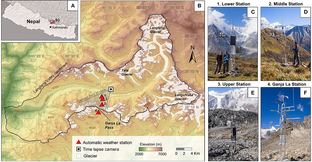
Figure 1. Study site location. (A) The location of Langtang Valley, Nepal. (B) Automatic weather station and time lapse camera location within the Langtang Valley catchment. Major glaciers and ice masses in Nepal are displayed (Bajracharya et al., 2014). The lower (C), middle (D), upper (E), and Ganja La (F) automatic weather stations in snow free conditions.

All four stations measure hourly air temperature (T_a) and humidity, ground temperature, snow depth, and have time-lapse cameras that take five images per day of the station surroundings. Liquid precipitation (rainfall) is recorded at three out of four stations. Moreover, the highest station (Ganja La), located on the south side of the Ganja-La pass (Figure 1), is also equipped with an extra precipitation gauge able to record solid precipitation (snowfall). In addition, SWE, air pressure, long- and short-wave radiation, as well as wind-speed and direction are recorded at the Ganja La station. Kirkham et al. (submitted) provide a detailed analysis and evaluation of the snow and solid precipitation related measurements from the Ganja La station. The sensors transmit their data in real-time via the Iridium satellite constellation. In addition to the four stations, a solar-powered high-resolution time-lapse camera was installed on the opposite side of the valley (Figure 1) in order to monitor the SCA and SLE on the mountain side where the four stations are located.

Since September 2015, hourly values of 41 different variables from the four stations have been transmitted in real-time, and the four stations have been operating 77–99% of the time. Despite some malfunction, always at least two of the four stations have been functioning well. The dataset obtained from September 2015 to June 2018 was processed further removing a few outliers, correcting snow depth for bare ground offset and aggregating the hourly values to 3 and 24-h means (sums for precipitation). An exception to the general hourly measurement rate is the SWE-sensor (Campbell Scientific CS725), which updates every 6 h its 24-h-averaged counts of gamma-radiation emitted from potassium isotopes (⁴⁰K) naturally contained in the ground, attenuated by snow. Due to the 24-h averaging of gamma-ray counts, the sensor's response to rapid changes in SWE is somewhat slow and delayed. The parallel hourly precipitation and snow depth measurement and CS725 data analysis by Kirkham et al. (submitted) showed an average delay time of 18 h. The SWE data used in this study are corrected for this lag. The CS725 at the Ganja La station, located at almost 5,000 m a.s.l., provides unique and valuable data to estimate solid precipitation (Kirkham et al., submitted) as well as the snow melt water contribution to runoff Q_M and the net snow melt rates M_obs (section Station Data Analysis and Estimation of Model Parameters).

We define a snow-covered period (t_SCP) for the Ganja La station as all the 3-h time steps from January 2017 to June 2018 (including the two major periods of seasonal snow cover) when the observed SWE is >15 mm and the observed surface albedo is >0.46. This definition is based on the time-lapse image analysis of the uniformity of snow cover at the Ganja La station by Kirkham et al. (submitted). In total, this definition provides 1,597 time steps with snow cover for our analysis, equivalent to 200 days. A verification check shows that 99% of the measured snow depth values in the t_SCP are between 9 and 88 cm.

MODIS Snow-Covered Area

Satellite imagery provides a high-resolution and spatiotemporally well-covering source of snow information. This is an especially valuable snow data source in remote high-mountain regions, such as the Langtang catchment.

We use the MODIS 8-day maximum binary (snow/no snow) SCA product with 500 m spatial resolution (1) for evaluating the model performance and (2) for comparing the SLE statistics between the Langtang region and other regions in Nepal. The SCA products from Terra (MOD10A2) and Aqua (MYD10A2) satellites acquire data in the morning and afternoon, respectively, and utilize the Normalized Difference Snow Index (NDSI). This is the ratio of difference and addition between the reflectance in visible (band 4, 0.545–0.565 μm) and short-wave infrared (band 6, 1.628–1.652 μm) wavelengths (Hall et al., 1995). A pixel is classified as snow if the NDSI ≥0.4 and the reflectance in band 2 (0.841–0.976 μm) and band 4 exceed 10 and 11%, respectively. Stigter et al. (2017) obtained a 83.1% classification accuracy for MOD10A2 product based on a comparison with field observations in the Langtang catchment.

The available data were further enhanced by reducing the number of cloud-covered pixels using the combined Aqua and Terra SCA products, followed by temporal and spatial filtering (Gurung et al., 2011). The temporal filtering fills cloud-covered pixels by cloud-free values from the previous and next 8-day time steps. The spatial filtering fills cloud-covered pixels by the most popular cloud-free values inside a surrounding 7 × 7 pixel window. Despite filtering cloud-covered pixels, the enhanced MODIS snow product is still significantly influenced by misclassifications of cloud cover as snow, particularly during the monsoon season (section Spatiotemporal Variation of the SLE Derived from MODIS SCA-Images, Model Simulation Results). Therefore, the monsoon season SCA-images (June-September) are omitted in this study (except in Figure 4A).

As snow cover is often patchy, it can be difficult to derive a distinct snow line which separates snow-covered terrain from snow-free areas. In this study we define the snow line as the zone where SCA gets below 0.5 (i.e., 50%). The SLE is estimated using the enhanced 8-day maximum MODIS SCA product and USGS HydroSHEDS elevation data (https://hydrosheds.cr.usgs.gov) resampled to the spatial resolution of MODIS using the nearest neighbor method.

In order to evaluate the representativeness of the SLE in the Langtang catchment for other areas of Nepal, the country's Himalayan region is divided into 50 × 50 km rectangular boxes taking Langtang Valley as the reference box (centered at Kyangjing village). All the SCA values within a box are assigned their respective elevation bands with 200 m intervals and a mean SCA for each elevation band is calculated. Finally, the SLE is defined as the highest elevation where the mean SCA, interpolated between the elevation bands, drops below 0.5 when moving from higher to lower elevations. The same SLE calculation method is also applied to the simulated SCA results from the seNorge model.

The seNorge Snow Model

Model Description

The snow simulation model applied in this study is the single-layer seNorge snow model (Saloranta, 2012, 2016), which was originally developed for operational snow mapping in Norway (www.seNorge.no). The high-mountain version (v.2) of the model, described in Saloranta et al. (2016), is applied here and its meteorological input data requirements are T_a and precipitation. The model is coded in the “R” statistical software (www.r-project.org), and consists of two main sub-models, namely: (1) the SWE sub-model for snow pack water balance and (2) the snow compaction and density sub-model for converting SWE to snow depth. The extended degree-day method (Hock, 2003; Pellicciotti et al., 2005) is applied to calculate snow melt rates M_eDD [mm h⁻¹].

$\begin{array}{ll}{M}_{eDD}=max(0,b_0{T}_a+c_{0}S{W}_{net}),if{T}_a>T_M& (1)\end{array}$

where SW_net is the net shortwave radiation flux [W m⁻²], b₀ [mm h^−1°C⁻¹] and c₀ [mm h⁻¹ (W m⁻²)⁻¹] are empirical snow melt parameters, and T_M is a melt onset threshold temperature parameter. The SW_net = (1–α_s)·SW_in, where the formulation by Allen et al. (2006) is used to estimate the incoming solar radiation SW_in for inclined grid cells with defined slope and aspect, taking also into account the attenuation in the atmosphere as well as the diffuse solar radiation. The snow surface albedo α_s is calculated as in Tarboton and Luce (1996), where α_s is a function of the solar angle, snow age and snow surface temperature. The snow melt rate for a grid cell is also affected by the simulated SCA in the grid cell, where the subgrid snow distribution is modeled using a uniform probability distribution function and a spatial snow variability parameter f_var (Saloranta, 2016). Negative melt rates are set to zero.

Refreezing of meltwater within the snowpack can occur in the model when M_eDD = 0 and T_a < 0°C. The model algorithm for refreezing of liquid water in the snow pack (Saloranta et al., 2016) is based on the “Stefan's law” model, originally developed for sea ice freezing (e.g., Leppäranta, 1993). In this approach, refreezing of liquid water is modeled in terms of a “refreezing front” which proceeds downwards from the top of the snow pack, effectively taking into account the fact that liquid water in the top layer refreezes much more easily than liquid water deeper in the snow pack, due to the thermal insulation effect of the snow. The temperature profile in the snow pack is assumed to be 0°C in wet snow below the refreezing front and linear above that, adjusting instantly to the changing snow surface temperature (approximated here by T_a). Whenever refreezing occurs, the increase in the depth of the refreezing front z_rf [m] in the snow pack is formulated as:

$\begin{array}{ll}{z}_{rf}^t=\sqrt{{\left(z_{rf}^{t-1}\right)}^2+\frac{{2\kappa }_s}{{\rho }_{lw}L}·(-T_a)\Delta t},if{T}_a<0^{°}C& (2)\end{array}$

where κ_s is the thermal conductivity of snow [W m⁻¹ K⁻¹], L is the latent heat of fusion [J kg⁻¹], ρ_lw is the partial density of the liquid water residing in the snow pack [kg m⁻³], Δt is the time step [s], and superscripts t and t–1 denote the current and previous time steps, respectively. The empirical parameterization for κ_s by Yen (1981) is applied, where κ_s = 2.22362·ρ_s^1.885, and ρ_s is the snow density expressed in [kg L⁻¹]. The z_rf is set to zero whenever liquid water from snow melt or rain enters the snow pack.

In order to simulate the integral effects of gravitational snow transport due to avalanching activity in steep Himalayan terrain, the SnowSlide algorithm Bernhardt and Schulz (2010) is applied. This algorithm was also used by Ragettli et al. (2015) and Stigter et al. (2017) in their modeling studies of the Langtang catchment. The algorithm distributes snow between grid cells whenever the slope angle S > 25° and a maximum snow holding amount SWE_max [mm] is exceeded. An exponential relation between S and SWE_max is applied as proposed by Bernhardt and Schulz (2010), where SWE_max = SS₁·exp(SS₂·S) (section Model Setup and Parameter Estimation).

Sublimation/evaporation from the snow pack is not implicitly calculated in the seNorge model, as this would preferably require distributed fields of wind speed and relative humidity as input forcing (Stigter et al., 2018). However, sublimation/evaporation from snow cover was recently estimated to be exceptionally high (21% of the annual snowfall) on the Yala glacier at 5,350 m a.s.l. in the Langtang catchment (Stigter et al., 2018). Consequently, a loss term for SWE at each time step due to sublimation/evaporation is included in the model code, and predefined sublimation/evaporation rates are provided as input for the model (section Model Setup and Parameter Estimation).

Model Setup and Parameter Estimation

The seNorge model (v.2) accommodates either 24 or 3-h simulation time steps. Observations of T_a in the Langtang catchment (section Snow and Meteorological Measurement Data) reveal high diurnal variability, where on 44–57% of all days (depending on the station) the minimum and maximum T_a are below and above the freezing point (0°C), respectively. Similarly, on 23–33% of all days, while the mean daily T_a is below the freezing point, the maximum T_a is above it. Consequently, the higher 3-h temporal resolution is selected for our model application as a daily model forcing time step would not be able to capture the frequent diurnal melt-refreeze cycles in the snow pack, as also pointed out by Ragettli et al. (2015).

A latitude-longitude grid with 15 arc s resolution (~450 m) is defined for the current model application for the Langtang catchment. The grid cell elevations are based on the Shuttle Radar Topography Mission (SRTM) digital elevation model (https://www2.jpl.nasa.gov/srtm/). The snow model application is started at July 1, 2016 at the approximate seasonal snow minimum (Immerzeel et al., 2009) assuming initial conditions simulated in a model spin-up run from July 2016 to July 2017. As the simulation period is 2 years, no yearly reset or removal of old snow/firn from the seasonal snow pack store is applied.

The main model parameters are listed in Table 1. Some of the parameter values depend on whether the grid cell is below or above the treeline, which is in our application approximated by the 3,000 m a.s.l. elevation contour. The sensitivity analyses of previous model applications in the Langtang catchment (Immerzeel et al., 2014; Ragettli et al., 2015; Stigter et al., 2017) indicate that the generally most influential model key parameters for simulated streamflow volumes, runoff and SCA are the correction factors and vertical gradients of precipitation and T_a, the threshold temperature T_thr for separating liquid and solid precipitation, as well as parameters related to snow melt algorithm (T_M, degree-day factor, fresh snow albedo). In our model application, many of these sensitive parameters, such as the vertical gradients of T_a, the threshold temperature T_thr, and the snow melt parameters T_M, b₀, and c₀, are estimated on the basis of relevant in-situ meteorological and snow observations in Langtang Valley, as described below.

TABLE 1

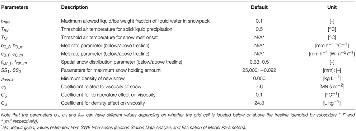
Table 1. The main seNorge snow model parameters with their default values.

The parameter value of T_thr used in the seNorge model is validated by examining measured T_a during snowfall events at the Ganja La station. Snow events are identified and confirmed using time-lapse camera imagery as well as snow depth and precipitation weighting gauge data (Kirkham et al., submitted).

The sublimation/evaporation rates R_SE [mm h⁻¹] from the snow pack will likely have a significant spatial variability in the Langtang catchment due to variability in wind speed and humidity. Due to the lack of such information, we cannot resolve the spatial distribution of R_SE in detail in our model application. In order to make a rough estimate of the influence of sublimation/evaporation at the catchment scale, we assume time-variable R_SE, which is constant in space. We estimate R_SE for the Ganja La station based on the bulk-aerodynamic method, as described in Stigter et al. (2018), and hourly in-situ meteorological data available at this site. We assume that the estimated time series of R_SE for the Ganja La station apply for all snow-covered grid cells in the catchment. We apply the surface roughness length for momentum (0.013 m) estimated by Stigter et al. (2018) and truncate the surface temperature to values ≤ 0°C (i.e., implicating presence of snow cover) allowing year-round estimation of R_SE at the Ganja La station.

A constant ρ_s of 0.270 kg L⁻¹ is assumed in the refreezing algorithm (Equation 2), based on field observations of the density of the upper 20 cm portion of the snow pack at its seasonal peak by Kirkham et al. (submitted). The avalanching model parameters SS₁ and SS₂ (Table 2) are estimated on the basis of the graph in Bernhardt and Schulz (2010; their Figure 2B). The resulting SWE_max for different slope angles is shown in Supplementary Material (Figure S1) and compared to an alternative parameterization by Ragettli et al. (2015).

TABLE 2

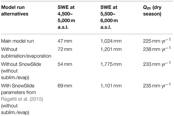
Table 2. Summary results for the main model run as well as for three alternative model runs, where no sublimation/evaporation is taken into account, and where in addition the SnowSlide avalanching routine was switched off, or where alternative SnowSlide parameter values (SS₁, SS₂) from Ragettli et al. (2015) were used.

FIGURE 2

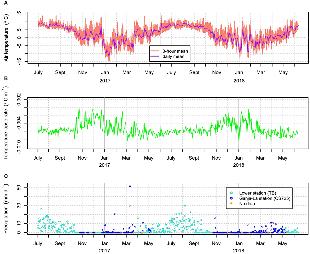
Figure 2. Model input forcing time series for the Lower station (4,200 m a.s.l.) from July 2016 to June 2018. (A) The daily and 3-hourly mean air temperature; (B) the daily mean temperature lapse rate, based on the air temperature difference between the Lower and Ganja La stations; (C) the daily precipitation data based on the Lower (tipping bucket, TB) and Ganja La (SWE-sensor, CS725) stations, respectively. The 4% of missing precipitation data (for which zero precipitation is assumed) is indicated by orange circles.

The snow model melt parameters T_M, b₀, and c₀ are estimated from observation-based snow melt rates (M_obs) in the t_SCP at the Ganja La station. A decrease in SWE registered by the CS725 implies that a corresponding amount of water in liquid or solid phase has left the snow pack either at the surface (i.e., evaporated/sublimated or blown away by wind) or through the bottom (i.e., runoff and percolation away from the monitored ground surface area). Thus, M_obs can be estimated from decreases in SWE recorded by the CS725, but this requires correction of the time-series for (1) sublimation/evaporation losses and (2) removal of episodes related to wind-blown snow. In addition, (3) refreezing of melt water in the snow pack must be compensated for when estimating M_obs as the “same” snow has then to be melted multiple times before the melt water finally can leave the snow pack. The additional effects of capillary melt water attachment to and release from the snow grains are not corrected for when estimating M_obs from the CS725 time series, as their net effect is assumed to be minor in a wet melting snow pack. An increase in SWE, normally registered by the CS725 due to snow accumulation (Kirkham et al., submitted), is assumed to imply no snow melting.

As the value-resolution of the CS725 is 1 mm and its time resolution is based on 24-h averages updated every 6 h, the CS725 time series cannot resolve the generally low sublimation rates (< 1 mm d⁻¹) or the 3-h melt rates. Therefore, time series of accumulated M_obs are used in estimation of the model melt parameters, weighing equally the total melt amount and root-mean-squared-difference (RMSD) in the optimization function.

The sublimation time series (R_SE) used in estimating M_obs from the CS725 time series at the Ganja La station are the same as applied in the model (see above). The estimation of the refreezing rates R_RF [mm h⁻¹] is challenging since no observed time-series of R_RF are available from the Ganja La station, or from any other similar site to our knowledge. Field observations of the snow pack at the Ganja La station at the time of maximum SWE (30th of April 2018; Kirkham et al., submitted), however, revealed a basal ice layer making up 22% of the current SWE and suggesting a significant refreezing within the snow pack. We use here model-derived time series of R_RF (section Model Description, Equation 2) from a grid point representative of the Ganja La station, showing that 34% of total snow melt is refrozen.

Wind erosion episodes, omitted when estimating M_obs at the Ganja La station, are assumed whenever the observed decrease of SWE is associated with 3-h-average of (hourly) maximum wind speed >8 m s⁻¹ over an erodible snow surface. An erodible, not melt-affected snow surface is assumed whenever the accumulated sum of positive degree-days is < 5 degree-days after the last snow fall. The wind speed threshold is the same as applied by Luijting et al. (2018), based on the empirical study by Li and Pomeroy (1997). This filter omits 22 mm (5%) of the observed decreases in SWE as wind erosion episodes.

Since most of the key model parameters are either set at default values or estimated from relevant observations, the model application is not additionally calibrated in this study against any SCA or snow depth observations. Consequently, the model application has not been fine-tuned specifically to work for the Langtang catchment only.

Meteorological Data for Snow Model Forcing

The meteorological input forcing data required for the seNorge snow model application are T_a and precipitation at each of the 3,084 simulated model grid cells in the Langtang catchment in the period from July 2016 to June 2018. This forcing data is, as described below, based on measurements of T_a and precipitation at the lowest (Lower) and highest (Ganja La) stations with an elevation difference of 760 m.

Air Temperature

The 3-h mean T_a values from the Lower, or if missing, from the Ganja La station are used to construct model input time series (Figure 2). This time series has < 1% of missing values which are estimated by interpolation. The T_a values from these stations are extrapolated to all the model grid cells in the Langtang catchment by using the corresponding grid cell elevations and the measured daily mean vertical gradient of air temperature (i.e., temperature lapse rate; Figure 2) between the Lower and Ganja La stations.

Liquid and Solid Precipitation

The precipitation input forcing data for the snow model (Figure 2) is a combination of 3-h-sum precipitation data from (1) the tipping bucket precipitation gauge at the Lower station and (2) data from the CS725 at the Ganja La station, updated every 6 h (Kirkham et al., submitted). The tipping bucket can adequately measure liquid precipitation only, and therefore its values are only used in the model forcing when the positive degree-day sum has exceeded 10 degree-days since the last recorded negative daily mean T_a, assuming this to ensure a gauge free of any snow and ice. The increases registered by the CS725 are utilized to estimate the solid precipitation (Kirkham et al., submitted) and therefore its values are only used in model forcing when T_a ≤ 0°C.

The precipitation time series from the Lower station tipping bucket gauge are adjusted up by 20% based on a measured difference in accumulated monsoon precipitation between the parallel tipping bucket and weighing gauges mounted on same mast at the Ganja La station (17 and 25% more precipitation in the weighing gauge in monsoon of 2016 and 2017, respectively). As the diameters of the orifices of the two gauges are the same, this difference could be connected to a larger wetting and evaporation loss from the walls of the tipping bucket. Since no wind measurements are available at the Lower station, wind-induced gauge catch-correction, as done by Kirkham et al. (submitted) for the gauge at the Ganja La station, is not feasible here. Fortunately, the wind-induced undercatch for liquid precipitation is generally small as compared to that of solid precipitation (Wolff et al., 2015).

Since the CS725 represents a much larger measurement footprint area (>150 m²) compared to common precipitation gauges (< 0.05 m²) and registers the solid precipitation at the ground level, no precipitation catch-correction factor is required. Kirkham et al. (submitted) compared the accumulated solid precipitation from the CS725 and from a weighing precipitation gauge and concluded that the CS725 captures ~38% more precipitation than the weighting gauge on average, a difference that was largely attributed to wind induced undercatch of the weighting gauge.

The data from the tipping bucket and CS725 complement each other in the model forcing time series: if a precipitation measurement from the tipping bucket is not available, a value from the CS725 is then used. The 760 m elevation difference between the two stations means that the Lower station is normally several degrees warmer than the Ganja La station, which is favorable in reducing the missing value period when switching from the rain- to the snow-based precipitation measurements in the autumn, and vice versa in the spring (Figure 2). The 4% of missing values in the period July 2016 to June 2018 are set to zero (i.e., no precipitation assumed; Figure 2).

The time series of solid precipitation from the CS725 at Ganja La station is first extrapolated to the elevation of the Lower station (4,200 m a.s.l.) by applying the seasonal vertical precipitation gradients of 0.031–0.053% m⁻¹ estimated by Immerzeel et al. (2014) for Langtang Valley. This unified precipitation time series estimated for the Lower station is then extrapolated to all the grid cells in the Langtang catchment by applying a monthly climatological spatial precipitation pattern based on the Multi-Source Weighted-Ensemble Precipitation (MSWEP; Beck et al., 2017a,b; http://www.gloh2o.org) global historic dataset (1979–2016). The MSWEP data is downscaled to the model grid resolution by applying the seasonally varying vertical precipitation gradients estimated by Immerzeel et al. (2014). Figure S2 shows examples of precipitation from MSWEP and the downscaled precipitation distribution patterns.

Results

Station Data Analysis and Estimation of Model Parameters

The mean daily vertical temperature gradient from July 2016 to June 2018 estimated between the Lower and Ganja La stations is −0.0054°C m⁻¹ and the 10 and 90% percentile values are −0.0071 and −0.0032°C m⁻¹, respectively. These values agree well with the previous estimates for Langtang Valley by Immerzeel et al. (2014). Using the four season definitions in Immerzeel et al. (2014), the strongest vertical temperature gradients are in our data detected in pre-monsoon (−0.0065°C m⁻¹) and monsoon (−0.0060°C m⁻¹), while the post-monsoon and winter gradients are somewhat weaker, −0.0042 and −0.0048°C m⁻¹, respectively (Figure 2). In the study by Immerzeel et al. (2014) the strongest gradients in Langtang Valley were recorded in winter and pre-monsoon (−0.0058 and −0.0064°C m⁻¹, respectively).

Since the tipping buckets cannot properly register solid precipitation, no year-round time series of vertical precipitation gradients can be calculated from our station data. However, during the monsoon 2016 and 2017 the measured accumulated precipitation difference between the Lower and Upper stations correspond to vertical gradients of 0.041 and 0.029% m⁻¹, respectively. These gradients agree roughly with the monsoon season vertical precipitation gradient of 0.040% m⁻¹ estimated for Langtang Valley by Immerzeel et al. (2014).

The snowfall event analysis (Figure 3A), using 6-h data-averaging and based on both snow depth and SWE measurements, shows that 95% of the recorded snowfall events occur at T_a < 0.5°C. Accordingly, the T_thr is set to the default value of 0.5°C in the model application.

FIGURE 3

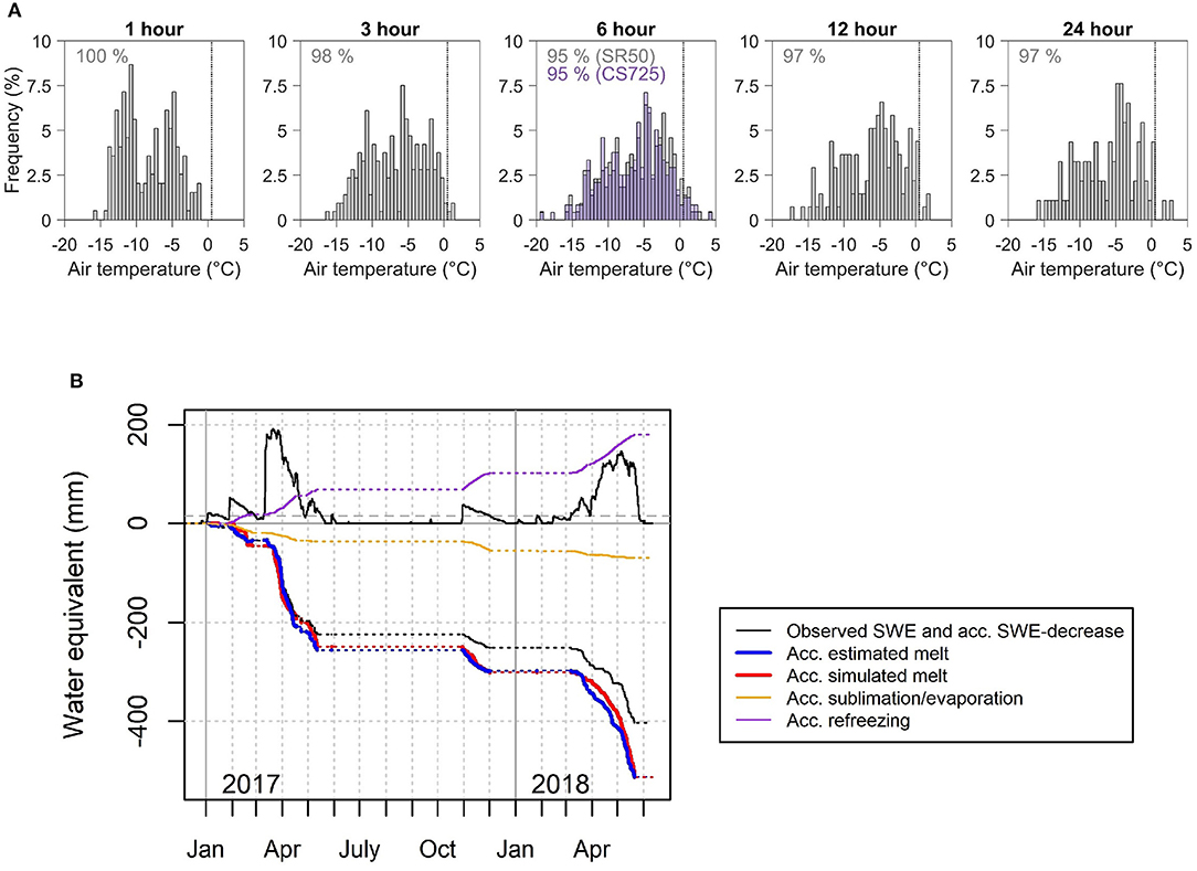
Figure 3. (A) Frequency distribution of ambient air temperatures at which snowfall occurs at the Ganja La station. The percentage of snow events that occur below the 0.5°C model temperature threshold is stated for 1, 3, 6, 12, and 24-h time windows. (B) Observed SWE and its accumulated (negative values) decrease at the Ganja La station (black lines) as well as the estimated (M_obs; blue line) and simulated (M_eDD; red line) accumulated snow melt during the snow-covered period in 2017–2018. The estimated accumulated sublimation/evaporation (orange line) and refreezing of melt water (purple line) are also shown. The gray dashed line denotes the lower limit of 15 mm SWE used in definition of the snow-covered period (t_SCP).

The mean of estimated daily R_SE at the Ganja La station in the t_SCP is 0.36 mm d⁻¹, while the 5 and 95% percentiles are −0.04 (deposition onto snow surface) and 1.1 mm d⁻¹, respectively. Evaporation comprises 25% of the R_SE. The whole time series of R_SE for the model simulation period (3-h values) is shown in Figure S3.

The time series of CS725 shows that in 27% of the days in the t_SCP, SWE decreases ≥3 mm d⁻¹ are recorded. Of these events the median and 95% percentile decreases are 5 and 12 mm d⁻¹, respectively, showing rather moderate daily decreases in SWE at the Ganja La station at an elevation around 5,000 m a.s.l. The total observed accumulated decrease of SWE in the t_SCP at the Ganja La station is 403 mm. The total accumulated R_SE in the same period is 70 mm, and the model-based estimate of refreezing indicates that ~34% of the total surface melt is refrozen within the snow pack at this site. Correcting the observed accumulated decrease of SWE for sublimation/evaporation (subtraction) and refreezing (addition) gives a net accumulated M_obs of 513 mm in the t_SCP (Figure 3B). The estimated sublimation/evaporation is thus 17% of the observed accumulated decrease of SWE and 14% of the estimated M_obs at the Ganja La station.

The 5, 50, and 95% percentile values of the snow melt model forcing variables (3-h means; Equation 1) at the Ganja La station in the t_SCP were −12.6, −4.8, +0.8°C for T_a, 0, 37, 244 Wm⁻² for SW_net and 0.72, 0.78, 0.80 for α_s. Moreover, the observed T_a and calculated SW_in are correlated somewhat, the correlation coefficient being r = 0.17 in the whole measurement period and r = 0.41 in the t_SCP (r = 0.45 if SW_net is used instead of SW_in). The calculated SW_in is strongly correlated with the observed SW_in (r = 0.81 in the whole period and r = 0.89 in the t_SCP), and even more with the observed incoming total radiation (short- and longwave radiation; r = 0.86 in the whole period and r = 0.92 in the t_SCP), as the decrease in SW_in due to clouds is partly compensated by increased atmospheric emissivity and thus increased incoming longwave radiation.

The 3-h values of the model melt parameters, optimized against the time series of accumulated M_obs (Figure 3B) are T_M = −3°C, b₀ = 0.33 mm (3 h)⁻¹ °C⁻¹ and c₀ = 0.0086 mm (3 h)⁻¹ (W m⁻²)⁻¹. The time series of simulated accumulated M_eDD matches well that of the observed M_obs (Figure 3B). The estimated b₀ and c₀ values for treeless terrain are assumed to apply also for the occasional snow cover in the lower-lying grid cells located below the treeline elevation of 3,000 m a.s.l.

When applying the optimized melt parameter values, the total amount of accumulated M_eDD in the t_SCP sums up to 514 mm (Figure 3B). If replacing the flat ground assumption at the Ganja La station by south and north facing slopes of 30° steepness, similar accumulated M_eDD values would be 7% higher and 33% lower, respectively, exemplifying the varying M_eDD along different terrain exposures to solar radiation in the Langtang catchment.

Spatiotemporal Variation of the SLE Derived From MODIS SCA-Images

The seasonal variation of the median SLE over the Langtang catchment (50 × 50 km box centered at Kyanjing village), as derived from MODIS 8-day maximum SCA-images, ranges from 3,075 to 5,341 m a.s.l., being lowest in February (Figure 4A) and rising gradually toward the monsoon season (July). A substantial variability of SLE occurs during the winter months (January to March). The low SLE outliers in Figure 4A in June-September are likely due to misclassification of clouds as snow (see e.g., Parajka and Blöschl, 2006).

FIGURE 4

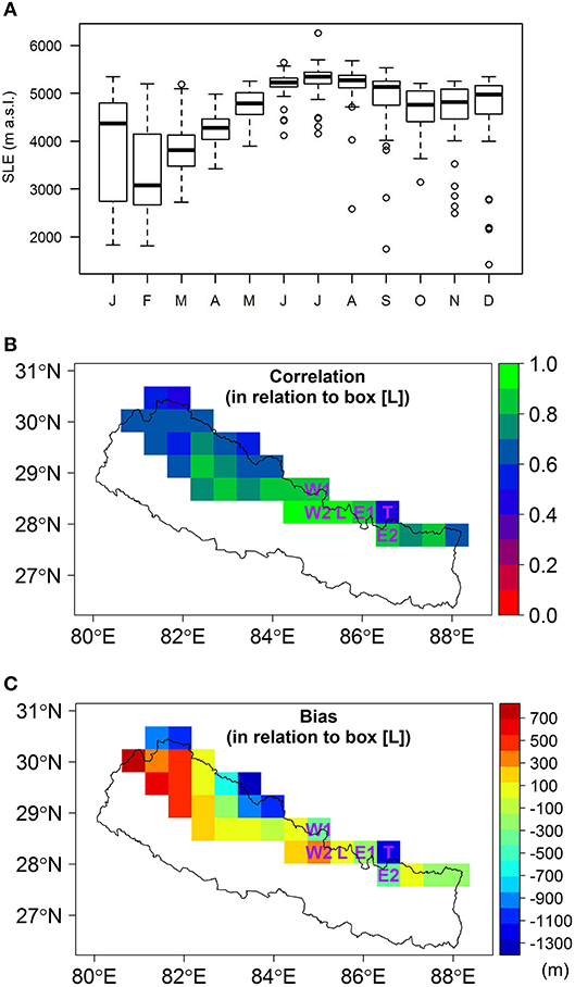
Figure 4. (A) Box-and-whiskers plot of the monthly distribution of observation-based SLE in 2001–2017 in a 50 × 50 km box over the Langtang catchment. The boxes and black line denote the 25 and 75% percentiles and the median, respectively. The whiskers denote the lowest and highest data point still within 1.5 times the interquartile range below and above the box. Data points outside the whiskers are denoted by circles. (B) Correlation and (C) bias of observation-based SLE time series between the 50 × 50 km box over the Langtang catchment (denoted by “L”) and 30 other similar rectangular boxes over the Nepal Himalayan region. Positive bias values mean a lower SLE than in the Langtang box. The letters indicate neighboring boxes toward the Tibetan Plateau (T), toward west (W1, W2) and toward east (E1, E2) of the Langtang box (L). All the SLE values are derived from MODIS satellite images (8-day maximum SCA).

Figures 4B,C show the spatial variability of correlation and bias for the observed SLE time series (monsoon season June-September excluded) between the Langtang box and other mountain areas of Nepal. No model results are thus used in this purely observation-based comparison. The correlation remains relatively high and bias low in many of the neighboring boxes to Langtang. For example, the neighboring boxes toward west and east (denoted by W1–W2, E1–E2 in Figures 4B,C) have correlation and bias values ranging from 0.80 to 0.92 and from −379 to +293 m, respectively, while the box just east of E1 toward the Tibetan Plateau (denoted by T in Figures 4B,C) has lower correlation and higher bias, 0.48 and −1,154 m, respectively. Regionally, the correlation gets weaker and the bias increases especially toward the central and far-western areas of Nepal. The most negative biases (higher SLE) are seen in the boxes located toward the drier Tibetan Plateau north of Nepal, while the most positive biases (lower SLE) are seen in the far western areas of Nepal (Figure 4C). The median of SLE correlation values for all boxes is 0.7 and the median bias close to zero, indicating that the Langtang box represents average SLE conditions in the Nepal Himalayas.

Model Simulation Results

The model results for snow depth, SLE and SCA in the simulation period July 2016–June 2018 are plotted together with observations in Figures 5, 6. An example illustrating a simulated SWE map for the Langtang catchment is shown in Figure 5A. The simulated snow depth at a grid cell between the Lower and Middle as well as between the Upper and Ganja La stations show generally a good match with the observed snow depth time series at these stations (Figure 5B). This figure also reveals some significant differences between the observed snow depths at the Upper and Ganja La stations, only 74 m apart in vertical and 2 km in horizontal distance, exemplifying the small-scale variability in point-based snow depth measurements (Lehning et al., 2008; Clark et al., 2011).

FIGURE 5

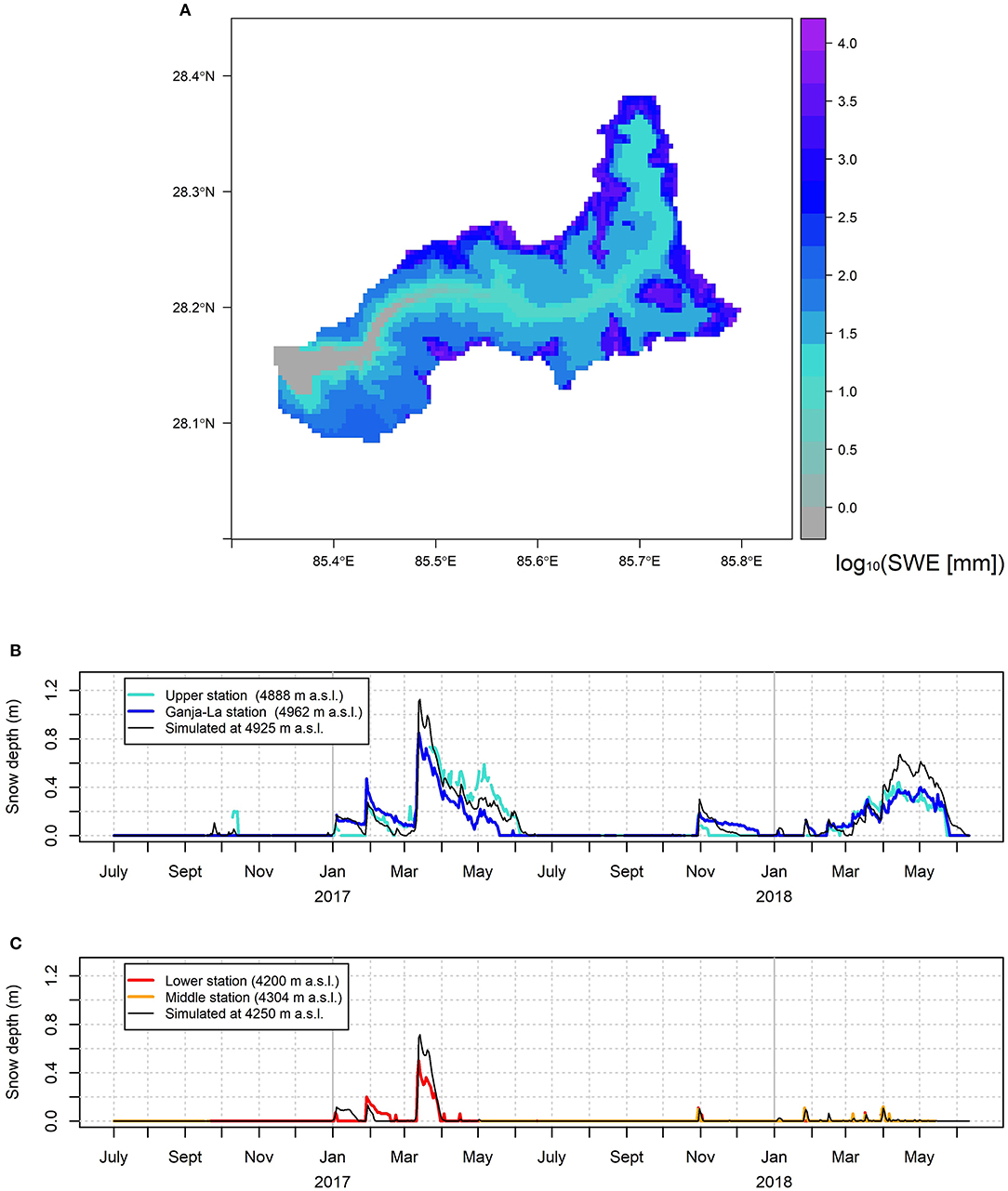
Figure 5. (A) Example of a simulated SWE map (log₁₀-transformed SWE-values) for the Langtang catchment in October 30, 2017. The observed snow depth from July 2016 to June 2018 (B) at the Upper and Ganja La stations and (C) at Lower and Middle stations. The simulated snow depth in a grid cell between the station-pairs is shown by black lines.

FIGURE 6

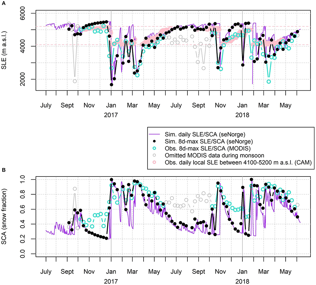
Figure 6. Time series of observed and simulated (A) snow line elevation (SLE) and (B) fraction of snow-covered area (SCA) in the Langtang catchment. Observations are based on MODIS 8-day maximum values (light blue circles), and the omitted dubious monsoon data in June-September is indicated by gray circles. The locally observed SLE on the north mountain face seen by the time-lapse camera (CAM; Figure 1) is shown in (A) by pink circles and the detectable SLE value range 4,100–5,200 m a.s.l. by horizontal pink dashed lines. Both daily (at 06:00 am, purple line) and 8-day-max (black circles) values of the model-simulated SCA and SLE are shown.

While the comparison to the snow depth measurements at the four stations in Figure 5B gives a useful confirmation of the model performance at two individual sites close to the origin of the model forcing data, the comparison to the observed average SLE and SCA in the Langtang catchment derived from MODIS satellite images provides a more comprehensive and catchment-wide evaluation of the model performance, despite of the inherent uncertainties in the satellite-based SCA estimates too (mostly due to misclassification of clouds as snow). This comparison (Figure 6) shows a reasonable overall model fit with the observations (8-day-maximum SCA). The mean model bias (simulated minus observed) for SCA and SLE is −7 percentage points and 110 m, respectively. The RMSD variability measure for model performance is 16 percentage points for SCA and 670 m for SLE. The manually derived SLE from the ground-based time-lapse camera (subjective estimates; the detectable value range is 4,100–5,200 m a.s.l.), viewing the mountain face where the four stations are located (Figure 1; Movie S1), agrees generally well with the MODIS-based SLE time series outside the monsoon season (Figure 6). However, during the monsoon season, the time-lapse camera images indicate generally much higher SLE than the MODIS-based estimates, justifying the omission of the monsoon season MODIS images from our analysis (section MODIS Snow-Covered Area).

The most relevant model results for any hydropower or water availability application would likely be the model-simulated accumulated water sources and stores, averaged over the Langtang catchment area (Figure 7). The all-year water sources from liquid precipitation P_liq and from snow melt Q_m are 1,046 and 426 mm yr⁻¹, respectively. However, if only considering the drier 8-months long non-monsoon period (October-May), Q_m becomes larger than P_liq (225 vs. 169 mm yr⁻¹). Most of the snow melt water comes from rather recently settled snow, and only about 30% of the snow melt water originates from snow older than 30 days (Figure 7A). The fraction of refrozen snow melt water is 36 and 48% during the all-year and the drier non-monsoon periods, respectively. The estimated accumulated sublimation/evaporation from the snow cover is lower in the all-year than in the non-monsoon period (57 vs. 69 mm yr⁻¹) due to deposition of water vapor onto snow cover during the humid monsoon.

FIGURE 7

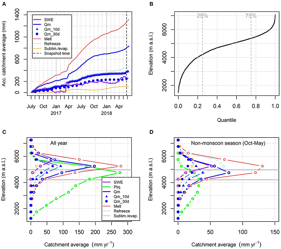
Figure 7. (A) Simulated accumulated snow-related water sources, stores and losses [mm, mean over the Langtang catchment] from July 2016 to June 2018. (B) The cumulative area-fraction vs. elevation distribution in the Langtang catchment. (C,D) As in (A) but now based on a “snapshot” of the accumulated values at the end of May 2018 and shown in units [mm yr⁻¹] (catchment average) for each 500 m elevation band for the all-year (left) and drier non-monsoon periods (October-May; right panel; note the different scale on x-axis). SWE is the snow store, and P_liq and Q_m the rainfall and snow melt water sources, respectively. Q_{m_10d} and Q_{m_30d} are the snow melt water sources derived from >10 and >30 days old snow, respectively. The thin lines (melt, refreeze, sublim./evap.) denote the surface snow melting, refreezing of liquid water within the snow pack, and sublimation/evaporation from the snow pack, respectively. The 4,200–4,962 m a.s.l. elevation interval monitored by the four stations is indicated by the two horizontal gray lines in (C,D).

Figure 7C shows the distribution of the accumulated water sources and stores at different elevation bands (500 m elevation intervals; see the cumulative area-fraction vs. elevation distribution in Figure 7B) at the end of the 2-year simulation period. When considering the all-year values, P_liq clearly dominates below ~5,000 m a.s.l. having the largest contribution from the 4,500–5,000 m a.s.l. elevation band. Above 5,000 m a.s.l. the storage of water in form of SWE increases and Q_m is slightly larger than P_liq. Above 6,000 m a.s.l. the water sources and stores (averaged over the Langtang catchment) diminish rapidly due to the small areal contribution of these highest elevations to the total catchment area (Figure 7B). During the drier non-monsoon season, when P_liq is much reduced, Q_m is larger than P_liq above 4,000 m a.s.l. having a maximum contribution from the 4,500–5,000 m a.s.l. elevation band. The refreeze to melt ratio generally increases with elevation, and above ~6,000 m a.s.l. all the snow melt water is eventually refrozen back to ice in the model simulations (Figure 7C). The sublimation/evaporation has a maximum contribution from the 5,000–6,000 m a.s.l. elevation band.

Due to uncertainties in estimating the spatial distribution of sublimation/evaporation and the gravitational snow transport (avalanching) parameterization in the model, three alternative model simulations were run: (1) without sublimation/evaporation; (2) without the SnowSlide avalanching routine activated; (3) with alternative SnowSlide parameter values (SS₁, SS₂) from Ragettli et al. (2015). The results (Table 2) show that in the drier non-monsoon season, the exclusion of sublimation/evaporation leads to only a slight 6% increase in catchment-averaged Q_m. Moreover, while the SWE distribution with elevation is sensitive to the gravitational snow transport model, the magnitude of Q_m, do not change significantly in these alternative runs either.

Discussion

When searching for suitable models to be used in e.g., water management-related issues, there are many application-specific considerations to make (e.g., Saloranta et al., 2003). Basically, there is no standard universally “best” model, but whether a model is appropriate or not depends on the purpose it is used for. The setup for snow mapping application for remote high-mountain areas, described in this paper, features several elements which should promote and lower the threshold of model use in practical applications. These features include: near real-time data delivery, almost maintenance-free measurement station setup (minimum of two temperature sensors, tipping bucket and CS725), simplified modeling approach, precipitation distribution estimated from easily available climatology. Such “live” estimation of the seasonal snow cover, rainfall and snowmelt rates allows us to provide effectively up-to-date information for predicting hydropower production potential and possible flood risk, for identifying areas of avalanche risk and for forecasting seasonal meltwater supply patterns to people in high-mountain regions, where all of these things are generally poorly known.

The spatial SLE analysis using MODIS satellite images gives an indication of the large-scale validity and transferability of the SLE results obtained for Langtang catchment to other catchments in the region, from which no ground-based observations exist. The large scale east-west and north-south gradients in SLE in Figure 4 (lower SLE toward west, higher SLE toward north) correspond well to previously detected gradients of snow cover persistence, which can be associated with the large-scale winter precipitation gradients in the Himalayas (Immerzeel et al., 2009). As many of the high-mountain regions in central and eastern Nepal (east of ~83°E) show high correlation (>0.8) with the estimated SLE in the Langtang catchment, the results from Langtang may provide a reasonable rough approximation of the snow conditions for these areas too.

The specific limitations of a model depend, as pointed out above, on the purpose it is used for. However, one common limitation and need for future development in snow models is related to the uncertainty of input data. Reliable meteorological forcing data is a crucial but often undervalued element in hydrological modeling (e.g., Magnusson et al., 2015), and especially the uncertainties in estimation of precipitation directly affect the accuracy of the estimation of snow accumulation. The main uncertainty sources in estimating precipitation are often the measurement gauge undercatch issue and spatial variability. The passive gamma-radiation SWE-sensor (CS725) has been a central instrument in our monitoring setup, and has contributed to reducing the potentially substantial gauge undercatch uncertainties for solid precipitation, commonly encountered with traditional precipitation gauges for which additional in-situ wind measurements are required for proper catch correction (Mekonnen et al., 2015; Wolff et al., 2015) (Kirkham et al., submitted). The use of CS725 in combination with a tipping bucket precipitation gauge at lower elevation has provided us year-round time series of precipitation.

The spatial variability of precipitation is a difficult problem to address, especially in mountainous terrain as the few measurement stations will not be able to capture all the smaller scale variability in precipitation (Collier and Immerzeel, 2015). A combination of information from high-resolution numerical weather prediction models, observations (gauge undercatch-corrected by e.g., simulated wind data) and even precipitation-radar data would likely provide significantly improved precipitation fields for model input. However, such a data-assimilation system is not (yet) feasible in our case, as most of such near real-time data needed for this are lacking in the Himalayas.

Applying the spatial precipitation pattern in the Langtang catchment from the MSWEP climatology provides an easily available way to spatiotemporally extrapolate precipitation measurements from a station-site to the catchment, although its spatial resolution (10 × 11 km) cannot match e.g., the local high-resolution meteorological model (Collier and Immerzeel, 2015) applied in precipitation extrapolation by Stigter et al. (2017). The precipitation distribution patterns adequately represent the observed tendency of increased precipitation at the lower western parts of the Langtang catchment (Immerzeel et al., 2014; Collier and Immerzeel, 2015), which would not be captured at all by using vertical precipitation gradients alone (see Figure S2). It is worth noting that we did not apply any additional calibrated precipitation correction factors in the current study. Such factors are commonly applied in glacio-hydrological models to adjust the model input precipitation in order to achieve a better model fit with observations.

The small-scale variability in precipitation, not captured by the precipitation distribution patterns, is demonstrated for example by the differences recorded by the Upper and Ganja La stations, which are located approximately at the same elevation on either side of a mountain pass. Despite being only 2 km south of the Upper station, the Ganja La station measures 41 and 47% more accumulated liquid precipitation during the monsoon in 2016 and 2017, respectively. This local difference may be specific and associated to the southerly prevailing wind direction typical during the monsoon season (Kirkham et al., submitted). However, the Upper station is located on a slope downhill of a ridge, which is probably not an optimal location for representative precipitation observations.

At the hillslope scale (1–100 m) the snow is inhomogeneously distributed due to preferential deposition of precipitation and wind redistribution effects (Lehning et al., 2008; Clark et al., 2011). This smaller scale snow variability is taken into account by the subgrid (< 450 m) snow distribution model (section Model Description). On the catchment scale (100–10,000 m), the effects of wind redistribution and preferential deposition are commonly assumed to be less significant, and variability in snow distribution is now dictated more by the local weather conditions, i.e., by the variability in precipitation and its phase (liquid/solid) as well as in the available melt energy (Clark et al., 2011). The exact scale in the Langtang catchment, where the role of wind redistributing snow becomes insignificant is, however, difficult to measure and verify in practice.

Forcing the snow model with T_a and precipitation data from our two-station approach provided simulation results of snow depth, SLE and SCA which matched rather well with the satellite and ground-based snow observations. The main focus of this study has been seasonal snow cover. If full water balance calculations in the catchment would be required, obviously also water source from glacier melt and loss to evapotranspiration, as well as ground water dynamics should be simulated or estimated. Based on Figure 6B, the elevation of the Ganja La station at about 5,000 m a.s.l. seems to be representative of the simulated area-averaged peak contributions of snow melt and rain related water sources, as well as refreezing and sublimation in the catchment. The uncertainties connected to the unmeasured vertical precipitation gradient values at the highest elevation range above 5,000–6,000 m a.s.l. fortunately seem not to be very significant for the catchment-averaged water source estimates (Figure 6), as < 10% of the catchment area is above 6,000 m a.s.l. Above 6,000 m a.s.l. the snow is essentially permanent in high-mountain Asia (Hammond et al., 2018).

Significant uncertainties are related to the spatial distribution of the sublimation/evaporation rates and to the estimation of the avalanching parameters. However, the model experiment results in Table 2 fortunately show only a minor effect for the simulated snow melt water contribution from the Langtang catchment, when the avalanching and sublimation/evaporation models were omitted. While for the refreezing algorithm the only whole-domain assumption is a constant snow density, for the sublimation/evaporation rate a spatially constant (but time-variable) value is assumed in our model application. Sublimation/evaporation rates may be significantly elevated locally near ridges and in blowing snow (Stigter et al., 2018). However, we believe our estimation method provides roughly representative values to assess the catchment-averaged significance of sublimation/evaporation. Sublimation/evaporation is estimated to account for 17% of the detected decreases in SWE at the Ganja La station, which is comparable to the value of 21% of annual snowfall estimated for the Yala glacier on the northern ridge of Langtang Valley (Stigter et al., 2018). As pointed out above, the simulated catchment average sublimation/evaporation loss from the snow pack (69 mm yr⁻¹) in the drier non-monsoon season has only a minor effect on the melt water runoff Q_m (13 mm yr⁻¹ reduction in Table 2). The reason for this is that the sublimation peak contribution is on a higher elevation range than the peak contribution of Q_m (Figure 7C). In other words, sublimation/evaporation does not deplete the snow cover so much there where most of the melt occurs. As a majority of Q_m originates from rather fresh, less than a month-old snow, sublimation/evaporation does not have that much time to “act” on the relatively ephemeral snow below ~5,000 m a.s.l. The role of sublimation can naturally be different in another catchment with significantly different climate. In such cases at least representative wind speed and humidity data would be required for estimation of sublimation rates in a new seNorge model application.

The SnowSlide avalanching model algorithm is much simplified, and in addition to the uncertain parameterization of SWE_max (Figure S1), many of the key processes affecting the triggering of avalanches, such as the past and present weather conditions, are not taken into account in the model. Better automatic detection of avalanche activity from radar satellites (Eckerstorfer et al., 2017) may in the future help to improve such avalanching models for hydrological purposes.

Many of the seNorge snow model key parameters, that would otherwise had to be estimated from literature or calibrated, were estimated from the monitoring data available at our stations. While Kirkham et al. (submitted) used SWE-increases from the CS725 to estimate solid precipitation and snow accumulation, the recorded SWE-decreases from the same instrument were in our study used to estimate snow melt and ablation rates. Estimation of the melt parameters (Eq. 1) locally from dedicated snow measurements should increase the performance of such simplified melt models, as indicated in the snow model intercomparison study by Skaugen et al. (2018). Our b₀ and c₀ values [converted to hourly values: b₀ = 0.11 mm h⁻¹ °C⁻¹ and c₀ = 0.0029 mm h⁻¹ (Wm⁻²)⁻¹] were only roughly half of the calibrated values in Ragettli et al. (2015). This discrepancy could be simply connected to differences in model formulation, such as the use of a different albedo scheme and a predefined, relatively high T_M of +1°C applied by Ragettli et al. (2015). In our case the optimized values of b₀ and c₀ as well as the goodness-of-fit value were increasingly sensitive to T_M when its value is set above −3°C (Figure S4). Thus, care should be taken to ensure a good coherence between the applied T_M, b₀, and c₀ values in extended degree-day melt model applications.

Sublimation/evaporation and refreezing estimates are implicitly included in many sophisticated multi-layer land surface models, such as in the ISBA (Interaction Sol-Biosphère-Atmosphère) model study by Eeckman et al. (2017) in the eastern Nepal region. Our model study is, however, as far as we know, the first study in the Himalayan region to include a catchment-wide process-based parameterization of melt water refreezing in the snow pack and locally verified estimates (Stigter et al., 2018) of mass losses from snowpack to atmosphere by sublimation/evaporation in a simpler single-layer snow model. Refreezing seems to be especially significant in the Langtang catchment as 48% of the melt water is simulated to refreeze in the catchment in the drier non-monsoon period. Based on measurements and modeling on a Canadian temperate glacier with much higher snow accumulation (1,700 mm yr⁻¹) and melt (3,000 mm yr⁻¹) rates compared to the Ganja La station, Samimi and Marshall (2017) estimated that on the order of 10% of total melt water is “recycled” melting from refrozen melt water. They anticipated the importance of refreezing to be even much more significant in colder alpine environments. The revised refreezing algorithm (Equation 2) provided an improved parameterization to estimate refreezing in the snow pack, enabling us to omit the use of an uncertain degree-day parameter for refreezing, used previously e.g., by Konz et al. (2007), Saloranta et al. (2016) and Stigter et al. (2017). In fact, if values for this parameter would be estimated from the revised refreezing algorithm results for the Ganja La station (Equation 2; dividing simulated 3-h refreezing rate by the corresponding T_a), the 5 and 95% percentile range of the degree-day parameter for refreezing would span nearly over two orders of magnitude (0.003–0.159 mm °C⁻¹ h⁻¹), clearly demonstrating that this model parameter is rather ill-defined and that the thermal insulation effect of the snow should be taken into account when estimating the refreezing. A sub-daily model time step (3 h in our case) is essential to properly capture the diurnal melt-refreeze cycles.

Conclusions

We have described a setup for simplified operational monitoring and modeling of seasonal rainfall and snow distribution for remote high-mountain areas, which can deliver data for snow and water availability mapping all year round. The setup utilizes (1) robust and almost maintenance-free in-situ instrumentation with satellite transmission, (2) a freely available numerical snow model, and (3) estimation of model key parameters from local meteorological and snow observations as well as from freely available climatological data. These features should promote and lower the threshold of model use in practical applications.

The snow model, not specifically calibrated in our application, produces results which are in reasonable agreement with observed snow depth, SCA and SLE time-series in the Langtang catchment. The model results show slightly less snow than indicated by the satellite-based MODIS SCA-images (bias of −7 percentage points in SCA and 110 m in SLE). The RMSD variability measure between the simulated and observed (MODIS) snow cover is 16 percentage points for SCA and 670 m for SLE. As many of the high-mountain regions in central and eastern Nepal show high correlation (>0.8) with the estimated SLE in the Langtang catchment, the results may provide a first-order approximation of the snow conditions for these areas too.

The estimation of melt parameters and solid precipitation from passive gamma-radiation based SWE-sensor data, as well as the improved process-based parameterization and locally verified estimation of the significant processes of refreezing within, and sublimation/evaporation from the snow pack, are features which to our knowledge have not been previously applied in glacio-hydrological catchment models in the Himalayan region. The simulation results suggest that most of the snow melt water comes from rather recently settled snow, and only about 30% of the snow melt water originates from snow older than 30 days. The ratio of snow melt water refreezing to total snow melt is 36 and 48% during the all-year and the drier non-monsoon periods, respectively. A sub-daily model time step (3 h in our case) is essential to properly capture the diurnal melt-refreeze cycles. The estimated accumulated sublimation/evaporation loss from the snow cover is lower in the all-year than in the non-monsoon period (57 vs. 69 mm yr⁻¹).

Our simplified snow mapping approach should be able to provide useful and up-to-date information on snow cover, snow depth and water equivalent, as well as on weather conditions fit for the purposes and needs of e.g., hydropower companies, local authorities and other practical applications in remote high-mountain areas.

Author Contributions

TS designed the study and wrote the initial version of the manuscript. All authors provided additional text and figures and/or comments on the manuscript. TS setup and ran the model application and analyzed the model results. AT compiled and analyzed the MODIS satellite data. JK and IK provided the snowfall threshold temperature analysis and helped to optimize the input data. KM provided the timelapse camera image analysis and movie, and ES calculated the sublimation rate time series. KnM designed the measurement station setup, and AT, KM, KnM, and ML participated in initial station installation in Langtang in 2015. All authors participated in additional station maintenance and field work.

Funding

The modeling and monitoring activities were done as part of the Snow accumulation and melt processes in a Himalayan catchment (SnowAMP) project developed by the International Center for Integrated Mountain Development (ICIMOD), the Norwegian Water Resources and Energy Directorate (NVE), and the Department of Hydrology and Meteorology, Government of Nepal (DHM). This work was supported by ICIMOD's Cryosphere Initiative funded by Norway, and by core funds of ICIMOD contributed by the governments of Afghanistan, Australia, Austria, Bangladesh, Bhutan, China, India, Myanmar, Nepal, Norway, Pakistan, Sweden, and Switzerland. Research was also financially supported by the European Research Council (ERC) under the European Union's Horizon 2020 Research and Innovation Programme (grant agreement No. 676819) and The Netherlands Organization for Scientific Research (NWO) under the Innovational Research Incentives Scheme VIDI (grant agreement 016.181.308). The views and interpretations in this publication are those of the authors and they are not necessarily attributable to their organizations.

Conflict of Interest Statement

The authors declare that the research was conducted in the absence of any commercial or financial relationships that could be construed as a potential conflict of interest.

Acknowledgments

We would like to thank Trine Lise Sørensen, Dinkar Kayastha, and all others who supported us during fieldwork or provided the equipment that was required, as well as Kathmandu University and the Department of National Parks and Wildlife Conservation for facilitation of our research permits. We also thank the two reviewers for their good and constructive comments on the manuscript.

Supplementary Material

The Supplementary Material for this article can be found online at: https://www.frontiersin.org/articles/10.3389/feart.2019.00129/full#supplementary-material

References

Alam, F., Alam, O., Reza, S., Khurshid-ul-Alam, S. M., Saleque, and Chowdhury, H. (2017). A review of hydropower projects in Nepal. Energy Procedia 110, 581–585. doi: 10.1016/j.egypro.2017.03.188

CrossRef Full Text | Google Scholar

Allen, R. G., Trezza, R., and Tasumi, M. (2006). Analytical integrated functions for daily solar radiation on slopes. Agri. Forest Meteorol. 139, 55–73. doi: 10.1016/j.agrformet.2006.05.012

CrossRef Full Text | Google Scholar

Bajracharya, S. R., Maharjan, S. B., Shrestha, F., Bajracharya, O. R., and Baidya, S. (2014). Glacier Status in Nepal and Decadal Change from 1980 to 2010 Based on Landsat Data. Research Report 2014/2, International Centre for Integrated Mountain Development (ICIMOD), Kathmandu.

Barnett, T. P., Adam, J. C., and Lettenmaier, D. P. (2005). Potential impacts of a warming climate on water availability in snow-dominated regions. Nature 438:303. doi: 10.1038/nature04141

PubMed Abstract | CrossRef Full Text | Google Scholar

Beck, H. E., van Dijk, A. I. J. M., Levizzani, V., Schellekens, J., Miralles, D. G., Martens, B., et al. (2017a). MSWEP: 3-hourly 0.25° global gridded precipitation (1979–2015) by merging gauge, satellite, and reanalysis data. Hydrol. Earth Syst. Sci. 21, 589–615. doi: 10.5194/hess-21-589-2017

CrossRef Full Text | Google Scholar

Beck, H. E., Vergopolan, N., Pan, M., Levizzani, V., van Dijk, A. I. J. M., Weedon, G. P., et al. (2017b). Global-scale evaluation of 22 precipitation datasets using gauge observations and hydrological modeling. Hydrol. Earth Syst. Sci. 21, 6201–6217. doi: 10.5194/hess-21-6201-2017

CrossRef Full Text | Google Scholar

Bernhardt, M., and Schulz, K. (2010). SnowSlide: a simple routine for calculating gravitational snow transport. Geophys. Res Lett. 37:L11502. doi: 10.1029/2010GL043086

CrossRef Full Text | Google Scholar

Braun, L. N., Grabs, W., and Rana, B. (1993). “Application of a conceptual precipitation-runoff model in the langtang khola basin, Nepal Himalaya,” in Snow and Glacier Hydrology Proceedings of the Kathmandu Symposium, November 1992 (Kathmandu: IAHS Publ.), 221–237.

Google Scholar

Callaghan, T. V., Johansson, M., Brown, R. D., Groisman, P. Y., Labba, N., Radionov, V., et al. (2011). Multiple effects of changes in Arctic snow cover. Ambio 40, 32–45. doi: 10.1007/s13280-011-0213-x

CrossRef Full Text | Google Scholar

Clark, M. P., Hendrikx, J., Slater, A. G., Kavetski, D., Anderson, B., Cullen, N. J., et al. (2011). Representing spatial variability of snow water equivalent in hydrologic and land-surface models: a review. Water Resour. Res. 47:W07539. doi: 10.1029/2011WR010745

CrossRef Full Text | Google Scholar

Collier, E., and Immerzeel, W. W. (2015). High-resolutionmodeling of atmospheric dynamics in the Nepalese Himalaya. J. Geophys. Res. Atmos. 120, 9882–9896. doi: 10.1002/2015JD023266

CrossRef Full Text | Google Scholar

Eckerstorfer, M., Malnes, E., and Müller, K. (2017). A complete snow avalanche activity record from a Norwegian forecasting region using Sentinel-1 satellite-radar data. Cold Reg. Sci. Technol. 144, 39–51. doi: 10.1016/j.coldregions.2017.08.004

CrossRef Full Text | Google Scholar

Eeckman, J., Chevallier, P., Boone, A., Neppel, L., De Rouw, A., Delclaux, F., et al. (2017). Providing a non-deterministic representation of spatial variability of precipitation in the Everest region, Hydrol. Earth Syst. Sci. 21, 4879–4893. doi: 10.5194/hess-21-4879-2017

CrossRef Full Text | Google Scholar

Essery, R., Morin, S., Lejeune, Y., and Ménard, C. B. (2013). A comparison of 1701 snow models using observations from an alpine site. Adv. Water Res. 55, 131–148. doi: 10.1016/j.advwatres.2012.07.013

CrossRef Full Text | Google Scholar

Etchevers, P., Martin, E., Brown, R., Fierz, C., Lejeune, Y., Bazile, E., et al. (2004). Validation of the energy budget of an alpine snowpack simulated by several snow models (SnowMIP project). Ann. Glaciol. 38, 150–158. doi: 10.3189/172756404781814825

CrossRef Full Text | Google Scholar

Fujita, K., Inoue, H., Izumi, T., Yamaguchi, S., Sadakane, A., Sunako, S., et al. (2017). Anomalous winter-snow-amplified earthquake-induced disaster of the 2015 Langtang avalanche in Nepal. Nat. Hazards Earth Syst. Sci. 17, 749–764. doi: 10.5194/nhess-17-749-2017

CrossRef Full Text | Google Scholar

Grünewald, T., and Lehning, M. (2015). Are flat-field snow depth measurements representative? a comparison of selected index sites with areal snow depth measurements at the small catchment scale. Hydrol. Process. 29, 1717–1728. doi: 10.1002/hyp.10295

CrossRef Full Text | Google Scholar

Gurung, D. R., Amarnath, G., Khun, S. A., Shrestha, B., and Kulkarni, A. V. (Eds.). (2011). Snow-cover mapping and monitoring in the Hindu Kush-Himalayas. ICIMOD-report, International Centre for Integrated Mountain Development, Kathmandu, Nepal.

Google Scholar

Gurung, D. R., Maharjan, S. B., Shrestha, A. B., Shrestha, M. S., Bajracharya, S. R., and Murthy, M. S. R. (2017). Climate and topographic controls on snow cover dynamics in the Hindu Kush Himalaya. Int. J. Climatol. 37, 3873–3882. doi: 10.1002/joc.4961

CrossRef Full Text | Google Scholar

Hall, D. K., Riggs, G. A., and Salomonson, V. V. (1995). Development of methods for mapping global snow cover using moderate resolution imaging spectroradiometer data. Remote Sens. Environ. 54, 127–140. doi: 10.1016/0034-4257(95)00137-P

CrossRef Full Text | Google Scholar

Hammond, J. C., Saavedra, F. A, and Kampf, S. K. (2018). Global snow zone maps and trends in snow persistence 2001–2016. Int. J. Climatol. 38, 4369–4383. doi: 10.1002/joc.5674

CrossRef Full Text | Google Scholar

Hock, R. (2003). Temperature index melt modelling in mountain areas. J. Hydrol. 282, 104–115. doi: 10.1016/S0022-1694(03)00257-9

CrossRef Full Text | Google Scholar

Huang, X., Deng, J., Wang, W., Feng, Q., and Liang, T. (2017). Impact of climate and elevation on snow cover using integrated remote sensing snow products in Tibetan Plateau. Remote Sens. Environ. 190, 274–288. doi: 10.1016/j.rse.2016.12.028

CrossRef Full Text | Google Scholar

Immerzeel, W. W., Droogers, P., De Jong, S. M., and Bierkens, M. F. P. (2009). Large-scale monitoring of snow cover and runoff simulation in Himalayan river basins using remote sensing. Remote Sens. Environ. 113, 40–49. doi: 10.1016/j.rse.2008.08.010

CrossRef Full Text | Google Scholar

Immerzeel, W. W., Pellicciotti, F., and Bierkens, M. F. P. (2013). Rising river flows throughout the twenty-first century in two Himalayan glacierized watersheds. Nat. Geosci. 6, 742–745. doi: 10.1038/ngeo1896

CrossRef Full Text | Google Scholar

Immerzeel, W. W., Petersen, L., Ragettli, S., and Pellicciotti, F. (2014). The importance of observed gradients of air temperature and precipitation for modelling runoff from a glacierized watershed in the Nepalese Himalayas. Water Resour. Res. 50, 2212–2226. doi: 10.1002/2013WR014506

CrossRef Full Text | Google Scholar

Immerzeel, W. W., van Beek, L. P. H., Konz, M., Shrestha, A. B., and Bierkens, M. F. P. (2012). Hydrological response to climate change in a glacierized catchment in the Himalayas. Clim. Change 110, 721–736. doi: 10.1007/s10584-011-0143-4

PubMed Abstract | CrossRef Full Text | Google Scholar

Konz, M., Uhlenbrook, S., Braun, L., Shrestha, A., and Demuth, S. (2007). Implementation of a process-based catchment model in a poorly gauged, highly glacierized Himalayan headwater. Hydrol. Earth Syst. Sci. 11, 1323–1339. doi: 10.5194/hess-11-1323-2007

CrossRef Full Text | Google Scholar

Lehning, M., Löwe, H., Ryser, M., and Raderschall, N. (2008). Inhomogeneous precipitation distribution and snow transport in steep terrain. Water Resour. Res. 44:W07404. doi: 10.1029/2007WR006545

CrossRef Full Text | Google Scholar

Leppäranta, M. (1993). A review of analytical models of sea-ice growth. Atmos. Ocean 31, 123–138. doi: 10.1080/07055900.1993.9649465

CrossRef Full Text | Google Scholar

Li, L., and Pomeroy, J. W. (1997). Estimates of threshold wind speeds for snow transport using meteorological data. J. Appl. Meteorol. 36, 205–213. doi: 10.1175/1520-0450(1997)036<0205:EOTWSF>2.0.CO;2

CrossRef Full Text | Google Scholar

Luijting, H., Vikhamar-Schuler, D., Aspelien, T., Bakketun, Å., and Homleid, M. (2018). Forcing the SURFEX/Crocus snow model with combined hourly meteorological forecasts and gridded observations in southern Norway. Cryosphere. 12, 2123–2145. doi: 10.5194/tc-12-2123-2018

CrossRef Full Text | Google Scholar

Magnusson, J., Wever, N., Essery, R., Helbig, N., Winstral, A., and Jonas, T. (2015). Evaluating snow models with varying process representations for hydrological applications. Water Resour. Res. 51, 2707–2723. doi: 10.1002/2014WR016498

CrossRef Full Text | Google Scholar

Mekonnen, G. B., Matula, S., DoleŽal, F., and Fišák, J. (2015). Adjustment to rainfall measurement undercatch with a tipping-bucket rain gauge using ground-level manual gauges. Meteorol. Atmos. Phys. 127, 241–256. doi: 10.1007/s00703-014-0355-z

CrossRef Full Text | Google Scholar

Parajka, J., and Blöschl, G. (2006). Validation of MODIS snow cover images over Austria. Hydrol. Earth Syst. Sci. 10, 679–689. doi: 10.5194/hess-10-679-2006

CrossRef Full Text | Google Scholar

Pellicciotti, F., Brock, B., Strasser, U., Burlando, P., Funk, M., and Corripio, J. (2005). An enhanced temperature-index glacier melt model including the shortwave radiation balance: development and testing for Haut Glacier d'Arolla, Switzerland. J. Glaciol. 51, 573–587. doi: 10.3189/172756505781829124

CrossRef Full Text | Google Scholar

Pradhananga, N. S., Kayastha, R. B., Bhattarai, B. C., Adhikari, T. R., Pradhan, S. C., Devkota, L. P., et al. (2014). Estimation of discharge from Langtang River basin, Rasuwa Nepal, using a glacio-hydrological model. Ann. Glaciol. 55, 223–230. doi: 10.3189/2014AoG66A123

CrossRef Full Text | Google Scholar

Ragettli, S., Pellicciotti, F., Immerzeel, W. W., Miles, E. S., Petersen, L., Heynen, M., et al. (2015). Unraveling the hydrology of a Himalayan catchment through integration of high resolution in situ data and remote sensing with an advanced simulation model. Adv. Water Resour. 78, 94–111. doi: 10.1016/j.advwatres.2015.01.013

CrossRef Full Text | Google Scholar

Rohrer, M., Salzmann, N., Stoffel, M., and Kulkarni, A. V. (2013). Missing (in-situ) snow cover data hampers climate change and runoff studies in the Greater Himalayas. Sci. Total Environ. 468, S60–S70. doi: 10.1016/j.scitotenv.2013.09.056

PubMed Abstract | CrossRef Full Text | Google Scholar

Saloranta, T., Litt, M., and Melvold, K. (2016). “Measuring and modelling snow cover and melt in a Himalayan catchment: Instrumentation and model code setup in the Langtang catchment Nepal,” in ICIMOD Working Paper 2016/7 (Kathmandu: International Centre for Integrated Mountain Development).

Google Scholar

Saloranta, T. M. (2012). Simulating snow maps for Norway: description and statistical evaluation of the seNorge snow model. Cryosphere 6, 1323–1337. doi: 10.5194/tc-6-1323-2012

CrossRef Full Text | Google Scholar

Saloranta, T. M. (2016). Operational snow mapping with simplified data assimilation using the seNorge snow model. J. Hydrol. 538, 314–325. doi: 10.1016/j.jhydrol.2016.03.061

CrossRef Full Text | Google Scholar

Saloranta, T. M., Kämäri, J., Rekolainen, S., and Malve, O. (2003). Benchmark criteria: a tool for selecting appropriate models in the field of water management. Environ. Manage. 32, 322–333. doi: 10.1007/s00267-003-0069-3

PubMed Abstract | CrossRef Full Text | Google Scholar

Samimi, S., and Marshall, S. .J. (2017). Diurnal cycles of meltwater percolation, refreezing, and drainage in the supraglacial snowpack of Haig Glacier, Canadian Rocky Mountains. Front. Earth Sci. 5:6. doi: 10.3389/feart.2017.00006

CrossRef Full Text | Google Scholar

Shrestha, A. B., Agrawal, N. K., Alfthan, B., Bajracharya, S. R., Maréchal, J., and van Oort, B. (Eds.). (2015). The Himalayan climate and water atlas: Impact of climate change on water resources in five of Asia's major river basins. International Centre for Integrated Mountain Development (ICIMOD). GRID-Arendal and CICERO.

Google Scholar

Skaugen, T., Luijting, H., Saloranta, T., Vikhamar-Schuler, D., Müller, K., and Kolberg, S. (2018). In search of operational snow model structures for the future–comparing four snow models for 17 catchments in Norway. Hydrol. Res. 49, 1929–1945. doi: 10.2166/nh.2018.198

CrossRef Full Text | Google Scholar

Smith, T., Bookhagen, B., and Rheinwalt, A. (2017). Spatiotemporal patterns of High Mountain Asia's snowmelt season identified with an automated snowmelt detection algorithm, 1987–2016. The Cryosphere, 11, 2329–2343. doi: 10.5194/tc-11-2329-2017

CrossRef Full Text | Google Scholar

Stigter, E. E., Litt, M., Steiner, J. F., Bonekamp, P. N. J., Shea, J. M., Bierkens, M. F. P., et al. (2018). The importance of snow sublimation on a Himalayan glacier. Front. Earth Sci. 6:108. doi: 10.3389/feart.2018.00108

CrossRef Full Text | Google Scholar

Stigter, E. E., Wanders, N., Saloranta, T. M., Shea, J. M., Bierkens, M. F. P., and Immerzeel, W. W. (2017). Assimilation of snow cover and snow depth into a snow model to estimate snow water equivalent and snowmelt runoff in a Himalayan catchment. Cryosphere 11, 1647–1664. doi: 10.5194/tc-11-1647-2017

CrossRef Full Text | Google Scholar

Tarboton, D. G., and Luce, C. H. (1996). Utah Energy Balance Snow Accumulation and Melt Model (UEB), Computer Model Technical Description and Users Guide. Utah Water Research Laboratory and USDA Forest Service Intermountain Research Station. Available online at: http://hydrology.usu.edu/dtarb/snow/snowrep.pdf (accessed May 22, 2019).

Google Scholar

Viviroli, D., Dürr, H. H., Messerli, B., Meybeck, M., and Weingartner, R. (2007). Mountains of the world, water towers for humanity: typology, mapping, and global significance. Water Resour. Res. 43:W07447. doi: 10.1029/2006WR005653

CrossRef Full Text | Google Scholar

Wolff, M. A., Isaksen, K., Petersen-Øverleir, A., Ødemark, K., Reitan, T., and Brækkan, R. (2015). Derivation of a new continuous adjustment function for correcting wind-induced loss of solid precipitation: results of a Norwegian field study. Hydrol. Earth Syst. Sci. 19, 951–967. doi: 10.5194/hess-19-951-2015

CrossRef Full Text | Google Scholar

Yen Y. -C. (1981). Review of Thermal Properties of Snow, Ice and Sea Ice. US Army Cold Regions Research and Engineering Laboratory (CRREL), Report 81-10, Hanover, NH.

Google Scholar