Exploring Spatial Heterogeneity of Antarctic Sea Ice Algae Using an Autonomous Underwater Vehicle Mounted Irradiance Sensor

Introduction

A significant proportion of primary production in ice-covered oceans is associated with ice algal cells living within or attached to sea ice (Arrigo et al., 1997, 2010; Lizotte, 2001). Sea ice reaches a yearly maximum extent of 20 million km² of Antarctic waters (Holland et al., 2014) and conservative estimates attribute approximately 20% of primary productivity to algae that grow on or in sea ice (Arrigo et al., 1991; McMinn et al., 1999; Arrigo and Thomas, 2004). Sea ice algae are particularly important to marine ecosystems as they are a spatially constrained source of fixed carbon available to higher trophic levels during spring before the onset of significant pelagic productivity (Arrigo and Thomas, 2004; Flores et al., 2012; Kohlbach et al., 2017; Schaafsma et al., 2017). During ice break-up and melt, sea ice algae may also play an important role in the export of fixed carbon from the photic zone (Boetius et al., 2013) and potentially in seeding planktonic production in marginal ice zones (Mangoni et al., 2009).

The existence of patchiness on millimeter (Lund-Hansen et al., 2017) and meter spatial scales in sea ice algae is well known from traditional ice coring approaches (Rysgaard et al., 2001) and imagery obtained from divers (Mundy et al., 2007) and under-ice vehicles (Ambrose et al., 2005). Cimoli et al. (2017) provides a complete review of the spatial scales associated with ice algae and emerging observational techniques. This review highlights how the quantitative sampling of sea ice algal biomass using traditional ice coring methods remains a laborious and spatially constrained approach (e.g., Mundy et al., 2007; Campbell et al., 2015), that fails to resolve the distribution of sea ice algal biomass at larger (>100 m) spatial scales (Lange et al., 2016, 2017; Meiners et al., 2017). The lack of reliable broad-scale data on ice algae biomass distribution makes the contribution of algae to regional food webs difficult to quantify, and thus creates a problem when trying to model the potential consequences of climate-driven changes to sea ice dynamics on ecosystem functionality.

To fully understand sea ice ecosystem function, it is critical to develop techniques that capture measurements of the variability of ice algal distribution and abundance at appropriate spatial scales. Such techniques may include underwater vehicles equipped with irradiance sensors to spatially map the spectra associated with the presence of ice algae growing at the ice-water interface (e.g., Lange et al., 2016, 2017; Meiners et al., 2017). This technique relies on suitably sensitive sensor arrays deployed beneath the ice surface and development of robust correlation algorithms between the spectral irradiance data and algal biomass.

While radiative transfer models for sea ice bio-optics have been available for many years (Arrigo et al., 1991; Zeebe et al., 1996), the range of optical attributes that are needed to generate and validate such models are difficult to obtain. For these reasons, most attempts to link under-ice irradiance with biomass involve empirical modeling of relationships between under-ice irradiance spectra, ice and snow properties, and algal biomass (Mundy et al., 2007; Fritsen et al., 2011; Ehn and Mundy, 2013; Melbourne-Thomas et al., 2015; Lange et al., 2016). A variety of algorithms have been used in these investigations and normalized difference indices (NDI) have consistently emerged as the most successful to date (Melbourne-Thomas et al., 2015). A review of published NDI values shows prediction models with coefficients of determination values (R²) ranging from 0.64 to 0.89, with wavelengths in the 420–490 nm band, proving the most useful in field-based research (Melbourne-Thomas et al., 2015). Optical methods for estimating ice algal biomass have been attempted for Antarctic pack ice (Fritsen et al., 2011) and Arctic land-fast ice (Mundy et al., 2007; Campbell et al., 2015), Arctic pack ice (Lange et al., 2016), Antarctic land-fast ice (Wongpan et al., 2018), and in pack ice for two sectors of the Southern Ocean (Melbourne-Thomas et al., 2015). These applications have been individually successful on a regional scale but other large scale variations between ice types have confounded development of a “universal algorithm” to date.

Routine use of optical methods for estimating sea ice algal biomass would greatly benefit from under-ice vehicles equipped with optical sensors able to obtain spatially resolved estimates of biomass across a wide range of length scales. To meet this need there have been several deployments of spectroradiometers on remotely operated vehicles (ROVs) under sea ice (e.g., Nicolaus and Katlein, 2013; Lund-Hansen et al., 2018). ROVs are generally limited by the tether length, platform stability and vehicle positioning. To further develop this approach, we mounted a multispectral radiometer on an autonomous underwater vehicle (AUV) to be flown along pre-programmed transects of up to 500 m in length under sea ice in November 2014. In contrast to ROVs, AUVs provide a more stable platform capable of making measurements over longer distances with greater spatial precision (e.g., Doble et al., 2009). In this research, we present a spatially explicit dataset showing transmitted spectral irradiance at different wavelengths across three separate transects from a single deployment hole. We present algorithms used to convert optical data to estimated biomass concentrations, specific to our study site through correlation and regression analyses of a dataset comprising under-ice spectra and algal biomass estimates within the survey area collected from an ice coring survey. The survey region was first year, land-fast ice off of Cape Evans, Antarctica, selected because it is: (1) a relatively deep region (>220 m water depth) of McMurdo Sound; (2) is well known for its near uniform first-year ice; (3) exhibits dense algal growth; and (4) often has minimal snow cover (McMinn et al., 2000; Remy et al., 2008). All of these variables were anticipated to optimize the chances of a successful first attempt at documenting variability of ice algal biomass using our AUV-based approach.

Materials and Methods

Field Sampling

Field sampling was conducted in early November 2014 at Cape Evans, McMurdo Sound, Antarctica (77° 38.2 S, 166° 20.8 E) (Figure 1A). The study design involved AUV-based optical sampling along three transects (CE1, CE2, and CE3) radiating at about 50° to each other from the deployment hole. AUV-collected under-ice topography from these transects are shown in Figure 1B (after Lucieer et al., 2016). A concurrent ice-coring campaign occupied 15 stations close to the transects covered by the AUV (Figure 1B) and an additional 5 within a 3 km radius of the deployment hole (positions not shown). Ice coring stations were selected to avoid any multi-year ice inclusions, and were largely free of snow because the entire AUV survey region had nearly no snow cover. Sampling outside the AUV area and between transects included targeting of small patches of snow cover, thought to be from the previous winter, to provide a range of snow thicknesses for subsequent analyses to explore the relationship of snow and presence of chl-a. Water depth at the site was in excess of 100 m.

FIGURE 1

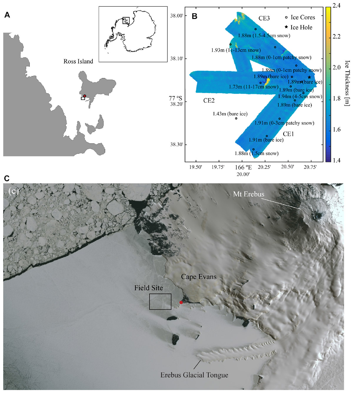
Figure 1. (A) Location of Cape Evans, McMurdo Sound within the Antarctic continent (inset); (B) Ice thickness as mapped across 60 m swaths using the interferometric Geoswath plus sonar onboard the AUV on the three transects where spectral irradiance measurements were made (CE1, CE2, and CE3) with point measurements of ice thicknesses and snow condition measured at each of the coring stations (open circle) in addition to the ice hole (filled star) from which the vehicle was deployed; and (C) a WorldView-1 satellite image collected on 2 November 2014 showing the snow coverage in the region around Cape Evans and the location of the main field camp (red dot).

Under-Ice Spectral Irradiance From Ice Coring

At each of the 20 ice coring stations (15 shown in Figure 1B) we deployed a spectroradiometer (TriOS Ramses ACC-UV/VIS cosine-corrected hyperspectral radiometer) with no pressure or tilt sensor, through a 250-mm diameter hole drilled through the sea ice after the AUV transects had been completed. The zenith angle was controlled by using a cable connected at the bottom of the sensor and the weight of the cable kept the sensor vertically positioned below the ice. This design was tested in a water tank in a laboratory before the field work. No data were excluded from the data-set and it was all corrected for the immersion effect. The light field below the ice is entirely diffuse whereby the effects of any possible tilt of the sensor is at a minimum.

The radiometer was mounted on an articulated arm that positioned the sensor 10–15 cm under the ice surface, 1.2 m from the outer edge of the access hole, to avoid the interference of light from the hole. The holes were also filled with snow and pieces of ice to avoid light interference. Transmitted spectra of downwelling irradiance (E_d, mW m⁻² nm⁻¹) had a nominal spectral resolution of 3.34 nm from 320 to 950 nm, though only values from 400 to 700 nm (i.e., photosynthetically active radiation – PAR) were used in this analysis. Once the radiometer was positioned under the ice, three replicate spectra were taken at each of three positions of the arm; toward the sun and at right angles left and right. All spectra were obtained under clear skies, within 4 h of solar noon. At each station, the exact position where each spectrum was obtained was marked on the ice surface. In addition, three incident spectra (E_d) were obtained above the ice surface. This was done by making 3 consecutive measurements of down welling irradiance in air immediately followed be 3 measurements of reflected irradiance at 50 cm above the ice. Spectrally resolved vertically downwelling attenuation coefficients [K_d(λ)] for the water column was estimated at one location by lowering the TriOS sensor to a maximum depth of 16.5 m and recording spectra at 1 m vertical intervals. Spectrally resolved vertical attenuation coefficients for downwelling irradiance [K_d(λ)] were calculated from these depth profiles using log-linear regression (Kirk, 2011).

Biological Parameters and Laboratory Analysis

At each of the ice coring stations, snow thickness was measured and an ice core was recovered from each of the three positions of the light arm using a 76 mm diameter SIPRE ice corer. Ice cores frequently had platelet ice frozen onto the bottom of the ice layer and were withdrawn with care to preserve as much of the platelet structure as possible, though at times some plates were dislodged. The thickness of the ice was measured for each core sample. Cores were photographed and the lower 50 mm of each, plus attached platelets, were cut off using a stainless-steel hacksaw, and transferred to a shore laboratory in a dark, insulated box for processing which occurred within 2 h of collection.

In the laboratory, ice core sections were thawed in the dark at 4°C for pigment analysis. Immediately after thawing, the final melt volume was measured and vigorously mixed to break up cell aggregates. Aliquots were filtered onto Whatman GF/F filters for: (1) chl-a, (2) other algal pigments (HPLC), and (3) absorption characteristics of the sea ice algae. Filters were stored individually wrapped and frozen in liquid nitrogen for up to 4 weeks during return to New Zealand or Denmark for longer term storage at −80°C.

To determine chl-a, filters were extracted in 95% ethanol and pigment concentration was determined using a Shimadzu UV2401 twin-beam spectrophotometer following Lund-Hansen et al. (2014). Phaeopigments were estimated by acidification, but no phaeopigment was detectable. One sample from the three chl-a samples at each station was selected at random for HPLC analysis. HPLC analyses were conducted on a Shimadzu HPLC equipped with an online photodiode array detector (SPD-M10Avp) and fluorescence detector (RF-10Axl) with excitation set at 350 nm and emission set at 450 nm (for identification purposes only). Injection of 25–100 μl was conducted using a Shimadzu SIL-10AF auto-sampler with sample cooler set at 4°C. A reverse phase Supelcosil LC-18 column (5 μm particle size; length 25 cm × 4.6 mm ID) with a guard column, was used for separation. Mobile phases used in the separation were 80:20 Methanol:0.5 M ammonium acetate, 90:10 Acetonitrile:UV-pure milli-q water and 100% ethylacetate. All chromatograms were integrated using Class VP 7.2 software. Identification of individual pigments was based on a combination of retention time and absorbance spectra, compared to commercial standards. Quantification of chlorophylls were based on absorbance at 662 nm and carotenoids at 449 nm. Here we focus on fucoxanthin (fuco), diadinoxanthin and xanthin (DDX), as dominant carotenoids within the sea ice diatom community. The concentrations of diatoxanthin and diadinoxanthin were added together (hereafter DDX) as these two pigments interconvert through epoxidation within cells. For comparison between samples, HPLC quantified pigments were normalized to chl-a.

Ice-Algae Absorption

Measurements of spectral absorption characteristics of the ice algae are based on a known volume of filtered ice melt collected onto a GF/F filter. We assumed that particulate absorption showed a similar spectrum as by the algae and did not measure particulate absorption. This might have introduced errors but these are considered to be minimum in light of the dominant chl-a absorptions. The filters were placed in front of the aperture of an integrating sphere attached to the Shimadzu spectrophotometer to measure absorption of wavelengths from 380 to 800 nm. The blank was a similar filter soaked in filtered seawater and the chlorophyll-specific absorption coefficient $a_{\mathrm{\lambda }}^{\ast }$ was subsequently defined as:

$$a_{\mathrm{\lambda }}^{\ast }=\left(2.303\cdot A_f/\left(\mathrm{\beta }\cdot V_f\cdot O{D}_{\mathrm{\lambda }}\right)\right)/\text{chl-a}\left(1\right)$$

where, A_f is the effective area of the filter (m²), V_f is the volume filtered (m³), OD_λ is the optical density of the filter at wavelength λ, β is a correction for path length amplification within the glass fiber filter (Cleveland and Weidemann, 1993), and chl-a is the estimated concentration of chlorophyll. The specific absorption coefficient $a_{\mathrm{\lambda }}^{\ast }$ was used in the optical modeling (see below) and normalized to $a_{672}^{\ast }$ to allow the shape of the algal absorption spectra from all samples to be compared (Lund-Hansen et al., 2014). The ice algae species composition was determined on Lugol-fixed samples and enumerated according to Uthermöhl (1958) and identified based on the work by Tomas (1997). More details are provided in Lund-Hansen et al. (2014).

Linking Under-Ice Spectra to Chl-a

Relationships between chl-a concentration and under-ice spectral irradiance measurements were then compared using two methods: (1) the normalized difference index (NDI), and (2) the empirical orthogonal function analysis (EOF). Three ice core samples and three L-arm surveys were carried out at each of the 20 stations, and each L-arm deployment consisted of three irradiance spectra that were averaged to give a total of 60 samples. The same methodologies and model selection criteria, with averaged triplicate TriOS spectra for each of the 60 samples as the input dataset (three samples for each of 20 stations), were used as detailed in Lange et al. (2016).

For the first method, a correlation surface matrix between all possible (301 × 301) NDI wavelength combinations, as the spectra were interpolated to 1 nm from 400 to 700 nm following Nicolaus et al. (2010), and the associated chl-a concentrations was generated with a moving average of a 3 × 3 nm grid centered at each value (e.g., Lange et al., 2016). This ensured that the maximum correlation value was not chosen at the edge of regions with an abrupt change between high and low correlations. The maximum correlation NDI wavelength combination was chosen with at least one wavelength within the range of 400 to 480 nm, which corresponds to the ∼440 nm chl-a absorption peak. A generalized linear model (GLM; McCullagh and Nelder, 1989) was constructed with chl-a concentrations and the maximum correlation NDI as the response and predictor variables, respectively. These took the log-link form defined in Eq. 2:

$$\ln \left(F\left(\text{chl-a}\right)\right)=\mathrm{\alpha }+\mathrm{\beta }(\text{NDI})\left(2\right)$$

where α is the intercept and β the regression coefficient. Consistent with Taylor et al. (2013) and Lange et al. (2016), we applied a log-link function for the prediction of chl-a [i.e., F(chl-a)] for both NDI and EOF GLM prediction models.

For the second method, a covariance matrix of the standardized spectra was submitted to an Eigen decomposition, which produces the EOF modes used as predictor variables. A GLM was constructed with chl-a as a response variable and the EOF modes and their squares as the predictor variables. Only the first 9 EOF modes, and their squares, were included to reduce the size of analysis and subsequently resulted in a total of 18 possible predictor variables. The “R” package glmulti (Calcagno and de Mazancourt, 2010) was applied to select the top 100 most reliable set of GLMs from all possible unique combinations. The bayesian information criterion (BIC) was used in the selection of robust models as it includes a penalty for both the number of predictor variables and the resulting estimated sample size (Schwarz, 1978). Finally, one reference model was selected based on the lowest BIC and in which all coefficients were significant (p ≤ 0.05). These GLM models have the following form defined by Eq. 3:

$$\ln \left(F\left(\text{chl-a}\right)\right)=\mathrm{\alpha }+{\mathrm{\beta }}_1{s}_1+{\mathrm{\beta }}_2{s}_2^2+\dots +{\mathrm{\beta }}_m{s}_m+{\mathrm{\beta }}_n{s}_{\mathrm{n}}^2\left(3\right)$$

where F(chl-a) is the log-link function for the prediction of chl-a, s_1,2,m,n are the EOF modes or the EOF modes squared from S determined from the GLM model selections, α is the intercept and β_1,2,m,n are the regression coefficients. In addition to determining the optimum NDI and EOF from the full suite of wavelength combinations available from the TriOS dataset to solve Eq. 3, we also undertook a limited analysis to focus on developing an NDI based on the wavelength data available from a multispectral cosine corrected radiometer (Satlantic OCR-507-ICSW) with 6 channels (412, 470, 532, 565, 655, and 670 nm) mounted on the AUV. The TriOS spectroradiometer-derived irradiance closest to the wavelength in the Satlantic bands was used in a pairwise fashion to derive all possible NDI values. Recognizing that the footprint of the AUV-mounted instrument was substantially larger than that of the ice corer or the TriOS itself, an averaged NDI for the three values measured at each of the 20 stations was used. These measurements were taken on the same day (although not concurrent) within a spatial distance of 1.7–2.4 m of each other. Likewise, we calculated average chl-a for the three cores from each station. We used a Pearson correlation to determine which NDI best predicted chl-a content.

Modeling Chl-a Concentration From Under-Ice Spectra

An unexpected feature was that the variability of chl-a concentration in the triplicate cores from each station was found to be higher than that of the chl-a concentration estimated from the corresponding irradiance spectra. To address concerns that we were failing to fully recover biomass from the fragile platelet component of the ice cores, a simple radiative transfer model was used with the specific goal of determining any evidence of undersampling of chl-a by coring. The iterative approach, modified from that of Mundy et al. (2007), was to use literature values of snow and ice spectral attenuation to first estimate, for each core, the spectral irradiance that would be expected under the ice, in the absence of algae. We then added in the effects of measured algal biomass using the chl-a concentration and $a_{\mathrm{\lambda }}^{\ast }$ for each site to develop a “predicted” under-ice spectrum. We then compared the predicted and observed spectra and, where they differed, iteratively changed the chl-a concentration used in modeling of the under-ice spectrum until the predicted most closely matched the observed. Observed and “required” chl-a concentrations could then be compared.

Specifically, following Mundy et al. (2007), we considered the sea ice was compartmentalized into snow, ice and ice/algae layer. Light entering this layer was estimated by subtracting measured reflectance from incident irradiance, and the attenuation by snow, then by ice, was based on attenuation coefficients for dry snow and cold ice given by Perovich (1990) and measured thicknesses. This allowed an estimate of the spectral irradiance reaching the ice/algae layer. To estimate the attenuation within the ice/algae layer (assuming no internal ice algae at this site) the approach of Ehn and Mundy (2013) was followed in Eq. 4:

$${\text{K}}_{\text{d}}(\mathrm{\lambda })\left(\text{ice}/\text{algae}\right)=1/{\mathrm{\mu }}_{\text{d}}\sqrt{\left[{\left({\text{a}}_{\mathrm{\lambda }}^{\text{ice}}+\text{C}\cdot {\text{a}}_{\mathrm{\lambda }}^{\ast }\right)}^2+0.238\left({\text{a}}_{\mathrm{\lambda }}^{\text{ice}}+\text{C}\cdot {\text{a}}_{\mathrm{\lambda }}^{\ast }\right)\left({\text{b}}^{\text{tot}}\right)\right]}\left(4\right)$$

where $a_{\mathrm{\lambda }}^{\text{ice}}$ is the wavelength-specific absorption coefficient (measured in m⁻¹) for ice taken from Perovich (1990), μ_d is the dimensionless average cosine of the downwelling hemisphere of the light field (taken as 0.7 after Ehn and Mundy, 2013), and b^tot is a scattering coefficient for ice taken as 413 m⁻¹ after Ehn and Mundy, 2013). C is the site specific chl-a concentration and a site specific $a_{\mathrm{\lambda }}^{\ast }$ that were used in these calculations and we assumed that the addition of algae to the ice did not change the scattering properties of the ice (Mundy et al., 2007; Ehn and Mundy, 2013). We iteratively changed the values of chl-a in these calculations until a least squares regression between observed and predicted irradiance was maximal across wavelengths from 400 to 600 nm (irradiance at wavelengths longer than 600 nm was too low to be included).

Autonomous Underwater Vehicle Irradiance Measurements

Irradiance measurements were made with a Satlantic OCR507 multispectral radiometer, along with its battery pack and a Satlantic STOR-X datalogger, mounted on a Gavia-class AUV (produced by Teledyne Gavia). The vehicle was pre-programmed to run three separate out and back 500 m return transects from a single deployment hole (recall lines CE1, CE2, and CE3; Figure 1C). As a result of the logistics of deploying, each transect was run approximately 2 h after the last. At a running speed of ∼1.5 m s⁻¹ and a sampling frequency of 25 Hz, this corresponds to a single measurement every 6–8 cm, although the cone of acceptance (i.e., the field of view) of the sensor meant that, at the depth of travel (∼6 m water depth), 75% of the irradiance sampled came from an under-ice footprint of approximately 4 m diameter. This water depth was selected as an estimated tradeoff between a safe operating envelope for the AUV and the quality of the collected data. The sampling frequency of the spectra data was subsequently downsampled to 1 Hz to match the navigation logging frequency of the vehicle.

Measurements of irradiance below the ice were collected at six, 10 nm wavelength bands centered on 412, 470, 532, 565, 625, and 670 nm. Known absorption properties of sea ice and ice algae suggested that attenuation of lower wavelengths (412–532 nm) would result from snow, ice and ice/algae whereas at 565–670 nm attenuation would primarily result from snow and ice (Hawes et al., 2012). To account for minor variations in AUV depth and ice cover thickness, the spectral irradiance at each wavelength was calculated for the ice-water interface using a vertical exponential attenuation model using data from the TriOS instrument deployments described above, and the water column length between the vehicle and the ice. Ice thickness was derived from collected sonar data and the recorded vehicle operating depth (Lucieer et al., 2016).

Statistical Treatment of Data

Relationships between snow, PAR transmittance (ratio of under-ice PAR irradiance to incident PAR irradiance represented as a percentage) and chl-a were examined using quantile regression analysis (QRA) techniques. QRA provides estimates of the relationship between the maximum chl-a concentration and snow depth, independent of data outliers and increasing/decreasing variance homogeneity over the snow depth range (Cade and Noon, 2003). Data were not transformed for QRA as it is a non-parametric test that makes no assumptions regarding normality of distribution or variance homogeneity.

To group samples by similarity of the spectral absorption of algae particulates on filters, a hierarchical cluster analysis based on $a_{\mathrm{\lambda }}^{\ast }$ normalized to $a_{672}^{\ast }$ was used through Primer 7. After grouping samples, snow cover, chl-a, fucoxanthin and DDX from sites within clusters were compared. As normality could not be established by transformation, non-parametric Mann–Whitney Rank Sum tests, within Sigmaplot 13, were run.

Correlograms were used to examine for spatial autocorrelation in the AUV-based NDI-derived estimates of chl-a along transects. Correlations were done based on offsets of 0–100 m, over transects of up to 475 m, and plotted Pearson’s correlation coefficient against offset distance to examine for periodicities in chl-a concentrations.

Results

Ice Coring

Across the study site, snow thickness was generally quite low (0–20 cm) with only one site having more (41 cm), and chl-a ranged from 9.7 to 81.7 mg m⁻² (Figure 2A). Concentrations of chl-a were log-normally distributed, with a geometric mean of 32.7 mg m⁻², and 95% C.I. of 11.4–62.5 mg m⁻². An apparent trend for high chl-a values under thinner snow depths was measured using QRA (Figure 2A), which became significant (p < 0.05) at the >80% quantile level. However, no simple relationship was found between transmittance, and chl-a (Figure 2B). The transmittance of total PAR through the ice varied between 0.12 and 0.90% of incident irradiance. This equates to 1.4–10.8 μmol photons m⁻² s⁻¹ at ice/ocean interface at a measured maximum surface irradiance of 1200 μmol photons m⁻² s⁻¹. As expected, thicker snow depth (up to 10 cm) tended to be associated with reduced transmittance, but further increases in snow thickness up to 40 cm made little further difference to the light transmittance (Figure 2C). These thicker snow patches tended to be only several meters in size, and horizontal transfer of scattered light within the ice may have enhanced irradiance under such patches. The snow patches were very compact and appeared to be old snow from the winter some months ago. Ice thickness varied little, ranging from 1.87 to 1.93 m, with the exception of a single station where a thickness of 1.43 m was recorded and no effect of ice thickness on transmittance was evident (data not shown).

FIGURE 2

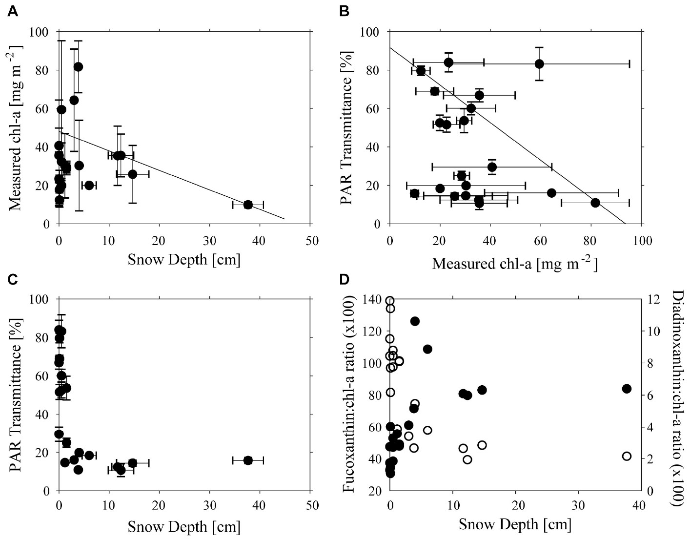
Figure 2. Relationships between (A) Snow Depth (cm) and chl-a concentration (mg m⁻²), (B) chl-a concentration (mg m⁻²) and PAR transmittance (%), (C) Snow Depth (cm), and PAR transmission (D) Fucoxanthin:chl-a ratio and Snow Depth (cm) (filled circles) and Diadinoxanthin:chl-a ratio (unfilled circles). Lines in (A,B) show significant 80% quantile regression lines and error bars are shown in (A–C).

As was expected, based on previous visits to the site, ice cores contained large amounts of platelet ice embedded on the underside of the sea ice. The ice algae occurred both within the congelation ice that was cementing the platelets into the ice, as well as associated with the platelets themselves. Despite care being taken to ensure that the core-platelet assembly was extracted as intact as possible, some biomass was likely lost. Differences in pigment composition with snow thickness were evident in responses of accessory pigments normally associated with light harvesting (fuco) and with light protection (DDX). The fuco:chl-a ratio increased toward a maximum value with increasing snow thickness, while DDX:chl-a ratio was low under thick snow cover and increased as snow decreased (Figures 2C,D). Ice-algae species were dominated by diatoms in all samples, particularly Fragilariopsis obliquecostata which represented 80% of abundances, with Nitzschia frigida and Navicula directa as subdominants.

Algal Absorption Spectra

Algal absorption spectra showed the typical large peak absorption by chl-a and carotenoids in the region of the blue wavelengths (400–500 nm) and a secondary chl-a peak at 665 nm (Figure 3 – Inset). Cluster analysis of normalized absorption spectra identified two distinct groups of core samples based on their absorption spectra, hereafter termed Group A (21 cores) and Group B (34 cores), with five outliers (Figure 3). The average absorption spectra of the two large groups differed only slightly, mostly in the 400 to 550 nm region (Figure 3 – Inset). These groups differed significantly in ratios of fucoxanthin and DDX to chl-a, with significantly higher proportions of photoprotective pigments in the low snow cover Group B, even though chl-a was similar in both groups (Table 1).

FIGURE 3

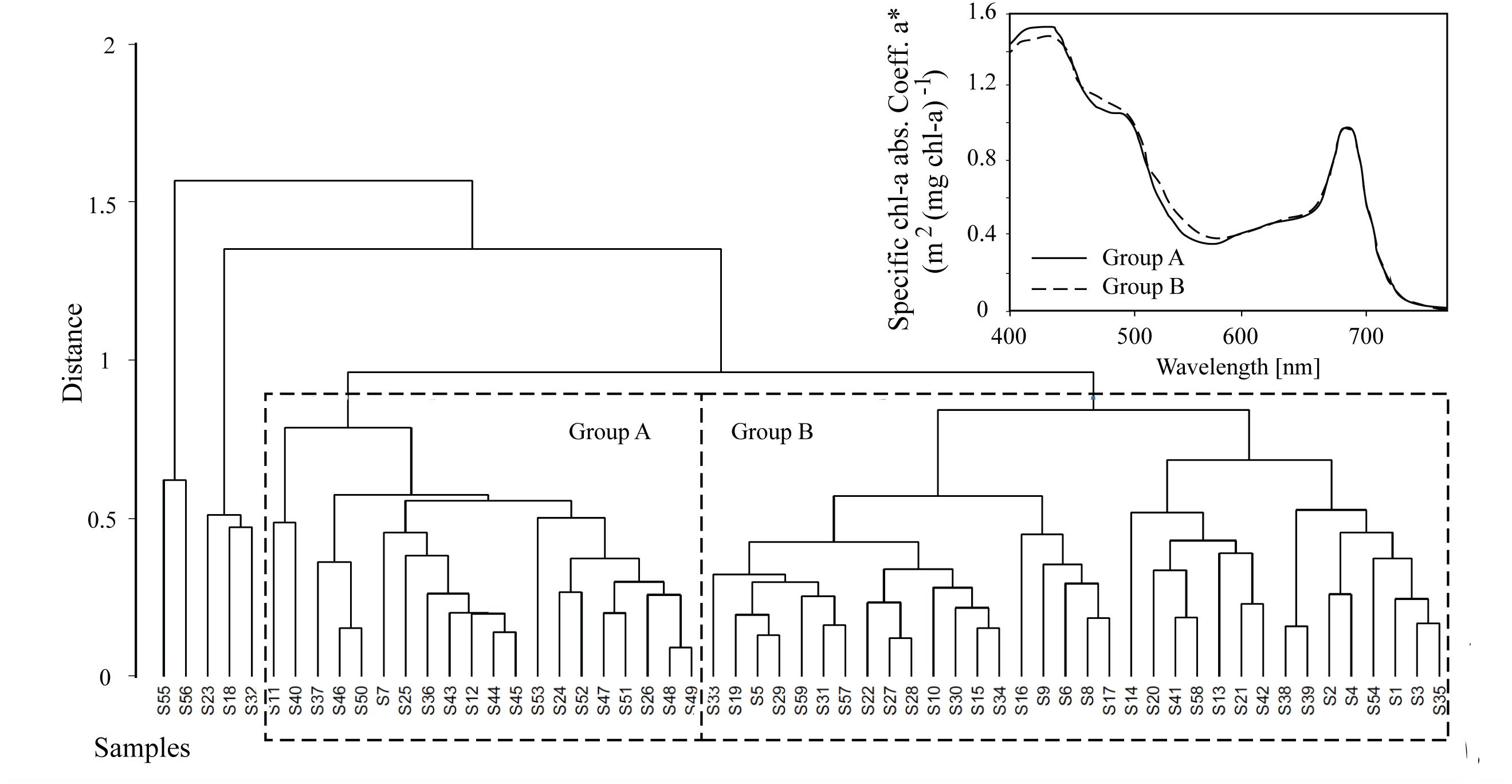
Figure 3. Hierarchical cluster analysis of absorption spectra from 60 samples where Groups A and B are shown for subsequent analysis. The average algae particulate absorption spectra normalized to the 670 nm peak for each of the two main Groups A and B is also shown for reference (inset).

TABLE 1

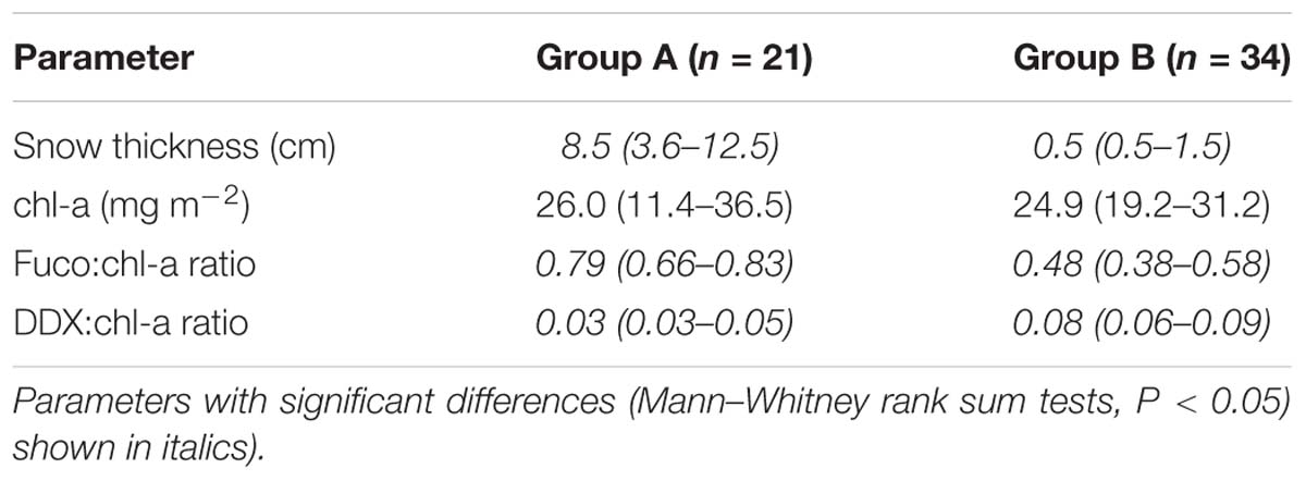
Table 1. Mean values (range in brackets) of snow thicknesses and pigment properties for the two groups of core samples identified by cluster analysis.

Estimations of NDI and EOF

Both empirical methods of linking under-ice spectra with measured chl-a explained a portion of the variance, but 95% prediction intervals were wide (Figure 4). The optimal combination of wavelengths for the NDI was 402:530 nm, which yielded a weak but significant coefficient of determination (R² = 0.31; p < 0.001) between predicted and observed chl-a (Figure 4A). The NDI residual showed no correspondence to snow cover, chl-a or to the two separate clusters of sites derived from $a_{\mathrm{\lambda }}^{\ast }$ analysis described below. The empirical orthogonal function (EOF, using modes S₂, S₃, and S₉) analyses produced a slightly better prediction of chl-a, (R² = 0.39; p < 0.001; N = 60), though the improvement on NDI was small (Figure 4B). As with NDI, examination of prediction residuals did not show a correspondence to snow cover, chl-a or site clustering.

FIGURE 4

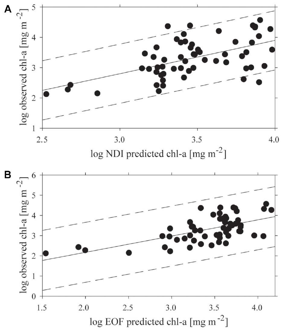
Figure 4. The relationship between predicted and observed chl-a concentrations (mg m⁻²) applying: (A) the normalized difference indices (NDI) 402:530 nm, and (B) the empirical orthogonal function analysis (EOF) both with a 95% confidence interval.

The NDI derived values using the restricted set of wavelengths, after averaging sites within stations, showed a significant correlation between ln(chl-a) and ln(NDI 412:532) (Figure 5). A predictive relationship of ln(chl-a) = 1.76⋅ln(NDI 412:532) + 5.30 was evident (R² = 0.47; p < 0.05; N = 18). NDI values were then estimated for each point along the AUV transects using the collected on-board Satlantic data, and this relationship used to estimate footprint chl-a. It should be noted that running the AUV at ∼6 m water depth translates to ∼4 m from the ice-ocean interface. Testing the sensitivity showed that errors in depth of ± 0.11 m identified by Lucieer et al. (2016) translate to a 0.3% error in estimation of NDI at the ice-ocean interface if a constant K_d(λ) is assumed. This assumption of a constant vertically downwelling attenuation coefficient across the study site was based on the fact that there were very short distances between coring sites and the AUV transects themselves were only a maximum of 500 m.

FIGURE 5

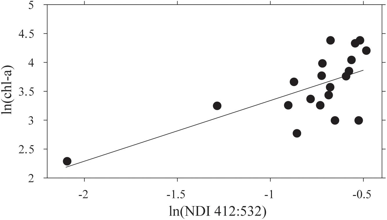
Figure 5. The relationship between ln(NDI 412:532) and ln(chl-a) for means of the three sample cores collected at each of 20 stations. The regression line fitted is ln(chl-a) = 1.05 ln(NDI)+4.39 (R² = 0.44; N = 20; F = 14.15; p = 0.001).

Modeling Chl-a Concentration From Under-Ice Spectra

Above the ice surface, all downwelling irradiance spectra were relatively constant (Figure 6A), but below the ice, distinctively shaped transmitted spectra, with lowered values between 400 to 550 nm and a dip at 670 nm were evident (Figure 6B). The modifications to spectra under ice were consistent with the areas of maximum absorption seen in algae particulates (Hawes et al., 2012). Synthetic under-ice spectra, derived from the model of ice and algae spectral attenuation, showed similar shaped spectra (e.g., Figure 6B). In the example given in Figure 6B, the optical model output was based on the measured chl-a and agreed well with the observed under-ice spectrum, but this was not consistent across all transects in this study. In most cases, the observed under-ice spectra could not be replicated using the measured chl-a to drive the model. In these cases, a close match between observed and modeled spectra was possible only by iteratively changing the chl-a concentration used in Eq. 4, to derive the chl-a concentration required to reproduce the observed spectrum. Required chl-a showed a similar range of average values across stations compared to measured chl-a, from 10 to 50 mg m⁻². Variance within each station was, however, much lower for required than observed values (Figure 6C). Three samples had similar modeled chl-a and measured chl-a concentrations (i.e., were in close proximity to the 1:1 line in Figure 6C), whereas required chl-a was larger than measured for nine of the samples, and lower than measured chl-a for six of the stations.

FIGURE 6

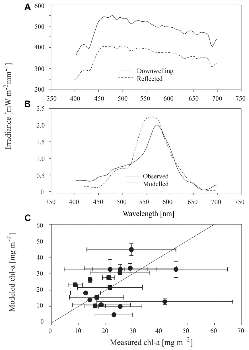
Figure 6. (A) Incident downwelling and reflected irradiance spectrum at the surface of sea ice at a representative sample site free of snow; (B) observed irradiance spectrum 10–15 cm underneath the sea ice, and modeled irradiance; and, (C) relationship between measured chl-a and modeled chl-a at the 18 stations for which sufficient data were available. Modeled chl-a is defined as the concentration necessary to reproduce the observed under-ice irradiance spectrum using the optical model. Points and bars are the mean and standard deviation of the three replicate samples at each of 20 stations and the solid black line is the 1:1 line between the two variables.

AUV-Derived Spatial Variability

Autonomous underwater vehicle measurements were made along CE1, CE2, and CE3 close to solar noon, with a repeat of CE1 being conducted 12 h later to examine diurnal variability. Each of these transects consisted of an out and back leg separated by ∼20 m. Examples of derived spatial variability in chl-a concentrations from repeat runs along transect CE1 at different incident irradiance at 23:45 04 November 2014 and 09:00 05 November 2014 (local times) are shown below (Figure 7A). The NDI derived chl-a using the established relationship (recall Figure 5) values agree closely at the spatial sampling scales, though the noise is enhanced in the run undertaken at midnight (local time), when the sensors were often approaching detection limits. Results from CE2 demonstrate the lack of relationship between minor variations in the first-year ice topography (shown in gray) and the observed variations in ice algae biomass (Figure 7B). While there is not enough evidence to be conclusive, there are reduced concentrations at the ice stalactite (observed ∼175 m along track) and increased concentrations around the greater ice thickness at around 360 m. Measurements along parallel tracks, approximately 20 m apart, show similar amplitudes and length scales of variation (e.g., CE3; Figure 7C) that would be expected to be poorly sampled using surface-based techniques. Average chl-a estimates from the AUV were lower than those from coring (18.7 vs. 26.7 mg m⁻²). We suggest that this is because the wavelength response of the multispectral Satlantic sensor does not follow that of the hyperspectral TriOS instrument and is integrating a larger footprint. In hindsight, the relationship between NDI and chl-a should be determined using the instrumentation to be deployed on under-ice vehicles. Nevertheless, we consider that the AUV provides a useful insight into spatial pattern of chl-a biomass in sea ice.

FIGURE 7

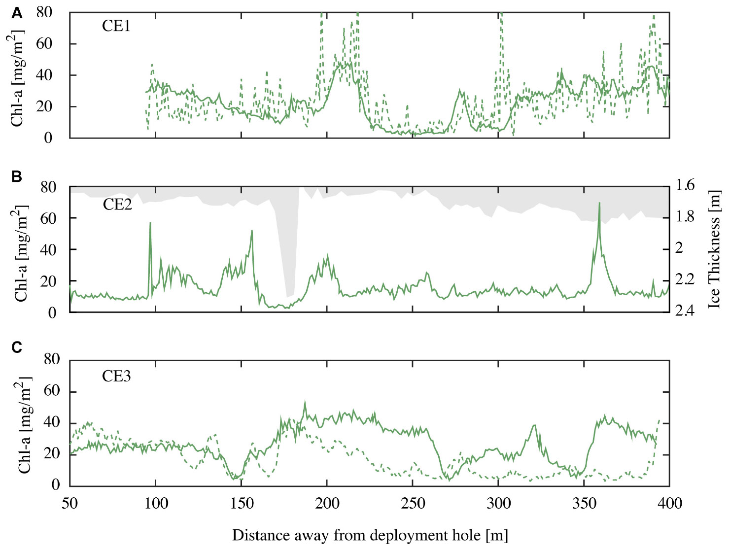
Figure 7. (A) Chl-a values for repeat runs of the outgoing transit leg of CE1 at local time 23:45 04 November 2014 (green dashed line) and 09:00 05 November 2014 (green solid line); (B) chl-a values for CE2 at local 10:45 05 November 2014 (green line) and overhead ice keel depth (bin averaged in 5 m intervals; grayed out) for the incoming transit leg; and (C) chl-a values for outgoing (green line) and incoming (green dashed line) transit legs (spaced at 20 m) for CE3 recorded at local time 09:45 05 November 2014.

Correlograms showed some degree of periodicity in estimated chl-a in most tracks, with apparent spatial autocorrelation length scales of 20–100 m for each of the transect runs (various colors; Figure 8). While the highest correlation is seen at the lower length scales (e.g., <20 m), longer length scales are evident in some of the transects (e.g., peaks of 50 and 110 m in the burgundy trace). The fact that these peaks were not evident in all of the data is an indicator of the spatial heterogeneity of these ice algal communities.

FIGURE 8

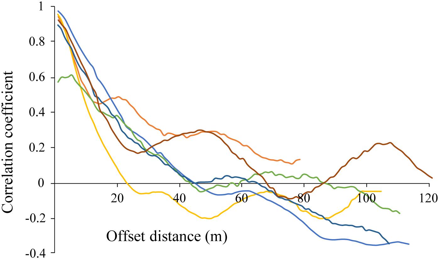
Figure 8. Correlogram for estimated chl-a derived from optical measurements made along each of the out and back AUV transects CE1, CE2, and CE3 (6 total; shown in individual colors). Repeat mission of CE1 at night not shown.

Discussion

The main purpose of this study was to develop a methodology to assess a compact, multispectral optical sensor, configured for AUV deployments for estimating spatial variability of sea ice algal communities. While similar approaches using an ROV and under-ice sleds have been demonstrated (e.g., Lange et al., 2016, 2017; Meiners et al., 2017; Lund-Hansen et al., 2018), this is the first attempt to our knowledge to make such irradiance measurements using an AUV. It is well documented that sea ice algae are optically active and make a significant contribution to the spectral attenuation in ice (e.g., Mundy et al., 2007; Ehn and Mundy, 2013; Melbourne-Thomas et al., 2015) making this type of remote sensing possible. Our data showed that it was possible to develop NDI and EOF correlations though with low correlations (R² = 0.31 and 0.39, respectively, N = 60) between predicted and observed chl-a, with broad 95% prediction intervals. These relationships are less reliable than previous studies, which developed predictive relationships with R²-values of up to 0.89 (see summary in Melbourne-Thomas et al., 2015) possibly due to the presence of platelet ice increasing the complexity of the ice structure where predictive relationships are weaker (e.g., R² = 0.07; Wongpan et al., 2018). When using the averaged values for each site to generate the NDI for use with the AUV, correlation was increased to R² = 0.41 (N = 19). A study based on radiance measurements below the platelet-rich ice in McMurdo Sound showed an even lower R² of 0.07 for correlation of NDI (471, 416) and chl-a concentrations (Wongpan et al., 2018). The relatively poor performance of the Wongpan et al. (2018) sampling was attributed to a relatively small range in chl-a that corresponded to a large change in optics, and the difficulty in sampling the fragile platelet ice, similar to our experience. Clearly this type of ice and location is relatively difficult for remote sensing. The difference in within-station variability between observed and required chl-a, and the high variance as observed by Wongpan et al. (2018) of measured chl-a may indicate the main reason for the inability of our EOF and NDI models to provide a robust prediction of biomass. Firstly, it is possible that biomass was playing a minor role in attenuation of light within the sea ice. This seems unlikely, as the spectral qualities of under-ice light showed distinctive shapes typical of sea ice algae, with rapid attenuation in the blue (440 nm) and red (675 nm), affected by chl-a and carotenoids (Fritsen et al., 2011).

A second possibility is that the fragile nature of the platelet ice that was present on site resulted in incomplete and variable collection of biomass. This would be consistent with the high variability in observed chl-a compared to observed under-ice spectra in station replicates. To address this possibility, we undertook the simple modeling exercise that compared the concentrations of chlorophyll observed with those required to reproduce the observed spectra. Estimation of missing parameters using optical models has previously been used by Mundy et al. (2007), who derived $a_{\mathrm{\lambda }}^{\ast }$ from under ice spectra, ice properties and chl-a biomass. In our case, we have independent estimates of $a_{\mathrm{\lambda }}^{\ast }$, and use these to estimate required chl-a to achieve observed spectra. This approach is limited by the sensitivity of such models to scattering (Ehn and Mundy, 2013). The scattering environment for ice with high amounts of embedded and extending platelets, as seen at Cape Evans, is poorly constrained and quantitative estimates of required chl-a may be difficult to achieve.

A third option thus relates to the footprint size of the irradiance sensor and the ice corer. While the core samples have a diameter of 75 mm, the TriOS spectroradiometer, would have an effective footprint diameter of 350–500 mm when positioned 100–150 mm below the ice (Nicolaus et al., 2010). The difference in sampling footprint size may be important in sea ice of the type described here, if a high degree of small-scale variability in biomass is related to the heterogenous matrix of the sub-ice platelet layer. The low variance in the required chl-a compared to measured chl-a for replicates at each station supports the view that, by sampling over a larger area, optical measurements are integrating variance, whereas under the conditions encountered at Cape Evans cores are not. Therefore, we suggest that when conducting these types of field observations under heterogeneous ice properties (i.e., a high probability of platelet ice) that multiple replicate cores are extracted from a region equivalent to the bottom-ice footprint size of the spectroradiometer.

Noise in the relationship between chl-a and NDI could be generated if there were substantial differences in the absorption spectra of ice algae across the sampling sites. However, while we did find significant differences between two groups of sites, the selected wavelengths did coincide with the selected NDI bands and differences were minor. These differences were systematic in that the two groups corresponded to sites with low (<5 μM photons m⁻² s⁻¹) and very low (<1 μM photons m⁻² s⁻¹) irradiances, and the shifts in carotenoid complements between these groups are consistent with a shift from energy harvesting (fuco) in low-light environments, to photoprotection (DDX) in higher light environments. Similar light-dependent carotenoid shifts have previously been reported in sea ice communities (Alou-Font et al., 2013). Robinson et al. (1997) also found that the diatoxanthin:chl-a ratio increased at higher irradiances in McMurdo Sound.

The shifts in absorption spectra and pigmentation of sea ice algal at Cape Evans occurred even though the highest light experienced by ice algae was low in absolute terms (e.g., average under-ice PAR was 2.61 μmol photons m⁻² s⁻¹). Models suggested that 1 to 23 μmol photons m⁻² s⁻¹ at a median incident irradiance of 720 μmol photons m⁻² s⁻¹ penetrated to the ice-algal layer, depending on snow cover. It is within, or slightly above, the range of previously reported critical minimum under-ice irradiance levels for algal growth of 2 to 9 μmol photons m⁻² s⁻¹ (e.g., Horner and Schrader, 1982; Gosselin et al., 1985, 1986; Lange et al., 2015). Active ice algae photosynthesis have recently been measured at 0.17 μmol photons m⁻² s⁻¹ (Hancke et al., 2018). In locations where ice and snow conditions allow a greater range of under-ice irradiance, more extensive divergence of pigmentation and absorption properties may be expected. We note that, while not significant in our study, this could potentially confound the development of NDIs based on carotenoid-specific wavebands, especially where there was a correlation between biomass, irradiance and carotenoids.

Our study region was dominated by a snow free ice cover with small snow patches (qualitatively observed to be <5 m) which did not alter the bottom-ice light levels below the snow patches due to the horizontal propagation/scattering of light from the surrounding snow-free regions. Because our study site was dominated by a snow free ice cover, there is a smaller decrease in the spatial coverage of sufficient bottom ice light levels for ice algal growth than expected. However, this finding has perhaps more significant implications for regions with thicker snow cover and less coverage of snow-free/thin-snow regions. In thicker snow regions the horizontal propagation of light may substantially increase the areal coverage of suitable light levels at the ice bottom around these sparse snow-free/thin-snow features. A future hypothesis to test is whether the scales of spatial variability in the algae compare to observed scales of snow cover.

If our failure to produce a robust NDI for use with the AUV data is due to the mismatch between footprint sizes of the ice corer and the spectroradiometer, our procedural difficulties relate to our calibration exercise rather than the performance of the AUV-mounted instrument. The AUV itself collected repeatable transects of multispectral optical data. NDIs can provide robust estimates of ice-algal biomass (Mundy et al., 2007; Fritsen et al., 2011; Melbourne-Thomas et al., 2015) and while our estimated chl-a concentration may have very wide confidence intervals, within the limitations of the large footprint of the AUV sensors, then patterns of variability of biomass seen at scales of several decimeters to meters appears to be reliable. Within this constraint, the observed pattern of spatial variation of biomass, with its patchiness on scales of 50–100 m, provides insight into the dynamics of sea ice algal communities and the design of sampling campaigns that need to be carried out to obtain area-representative samples. At Cape Evans, for example, the length scale of autocorrelation suggests that coring would need to be undertaken at ∼10 m intervals along 200 m transects to obtain adequate representation. The mechanisms underlying this broad scale pattern of biomass are as yet unclear. However, our data suggest that at present no single approach is adequate to fully understand multi-scale variability in sea ice algal biomass.

Conclusion

In this study, we endeavored to determine whether AUV-mounted sensors could obtain systematic, transect-based information on sea ice algae from their optical signature. To achieve this, we attempted to develop a predictive model linking the under ice irradiance spectra to the biomass of bottom-ice algae and then applied this to AUV-derived data. Such approaches are now well accepted, but, while we were able to show a statistically significant relationship (R² = 0.41), this had a higher prediction error than other models produced using similar approaches in other ice-covered environments. We found some variability in the absorption characteristics of ice algae due to shifting pigment complements but conclude that the most likely challenge to development of a robust algorithm may be the small-scale variability of ice algal biomass. This is a feature of sea ice algae in general, but is particularly acute in our example as the under-ice environment at Cape Evans provided a physically complex structure, where variable amounts of platelet ice were frozen into first year sea ice and formed part of the ice-algal habitat.

Optical methods to estimate ice-algal biomass produced a smaller variance than coring, which we suggest reflects its ability to integrate biomass over a larger footprint than coring. Thus, our results suggest that remote assessment of biomass based on optical properties may, with suitable calibration for local algal attenuation, provide an estimate of the ice algal resource over spatial scales that is more robust than coring approaches where small-scale variability of ice algal biomass is present. We used this approach, coupled to an AUV, to demonstrate what appear to be autocorrelated patterns of sea ice algal biomass on length scales of 10’s to 100’s m.

While sea ice imposes logistical challenges on the use of underwater technologies, the development of sensor arrays and the platforms that carry them offer a way forward to better understand sea ice algae communities. The development of such non-invasive techniques to measure environmental conditions under ice at scales commensurate with the inherent variability of these algal communities allows new understanding that would not be achievable with traditional methods and this alone represents a step change in our approach to studying these communities.

Author Contributions

All authors listed have made a substantial, direct and intellectual contribution to the work, and approved it for publication.

Funding

This work was supported by the Air New Zealand through the New Zealand Antarctic Research Institute (Project NZARI-2014-3). In addition, the authors would like to thank the ongoing support of the Danish Council for Independent Research (Project DFF – 1323-00335) and the Australian Research Council’s Special Research Initiative for the Antarctic Gateway Partnership (Project ID SR140300001). Griffiths University and the Defense Science and Technology Group (Australia) also contributed through equipment support. BL was partly funded during this study by a visiting fellowship from the Natural Sciences and Engineering Research Council of Canada (NSERC).

Conflict of Interest Statement

The authors declare that the research was conducted in the absence of any commercial or financial relationships that could be construed as a potential conflict of interest.

The reviewer PD declared a past co-authorship with one of the authors BS to the handling Editor.

Acknowledgments

We thank the Antarctica New Zealand for the provision of logistic support to ensure that this research was possible. Final thanks goes to Rowan Frost (Australian Maritime College Search) and the K081 Team for all of their work to make this project a success.

References

Alou-Font, E., Mundy, C. J., Roy, S., Gosselin, M., and Agustí, S. (2013). Snow cover affects ice algal pigment composition in the coastal Arctic Ocean during spring. Mar. Ecol. Prog. Ser. 474, 89–104. doi: 10.3354/meps10107

CrossRef Full Text | Google Scholar

Ambrose, W. G., von Quillfeldt, C., Clough, L. M., Tilney, P. V. R., and Tucker, T. (2005). The sub-ice algal community in the Chukchi sea: large- and small-scale patterns of abundance based on images from a remotely operated vehicle. Polar Biol. 28, 784–795. doi: 10.1007/s00300-005-0002-8

CrossRef Full Text | Google Scholar

Arrigo, K. R., Mock, T., and Lizotte, M. P. (2010). Primary producers and sea ice. Sea ice 2, 283–325. doi: 10.1002/9781444317145.ch8

CrossRef Full Text | Google Scholar

Arrigo, K. R., Sullican, C. W., and Kremer, J. N. (1991). A bio-optical model of Antarctic sea ice. J. Geophys. Res. 96, 10581–10592. doi: 10.1029/91JC00455

CrossRef Full Text | Google Scholar

Arrigo, K. R., and Thomas, D. N. (2004). Large scale importance of sea ice biology in the Southern Ocean. Antarctic Sci. 16, 471–486. doi: 10.1017/S0954102004002263

CrossRef Full Text | Google Scholar

Arrigo, K. R., Worthen, D. L., Lizotte, M. P., Dixon, P., and Dieckmann, G. (1997). Primary production in Antarctic sea ice. Science 276, 394–397. doi: 10.1126/science.276.5311.394

PubMed Abstract | CrossRef Full Text | Google Scholar

Boetius, A., Abrecht, S., Bakker, K., Beinhold, C., Felden, J., Fernandéz-Méndez, M., et al. (2013). Export of algal biomass from melting Arctic sea ice. Science 339, 1430–1432. doi: 10.1126/science.1231346

PubMed Abstract | CrossRef Full Text | Google Scholar

Cade, B. S., and Noon, B. R. (2003). A gentle introduction to quantile regression for ecologists. Front. Ecol. Environ. 1:412–420. doi: 10.1890/1540-9295(2003)001

CrossRef Full Text | Google Scholar

Calcagno, V., and de Mazancourt, C. (2010). glmulti: an R package for easy automated model selection with (generalized) linear models. J. Stat. Softw. 34, 1–29. doi: 10.18637/jss.v034.i12

CrossRef Full Text | Google Scholar

Campbell, K., Mundy, C. J., Barber, D. G., and Gosselin, M. (2015). Characterizing the sea ice algae chlorophyll a–snow depth relationship over Arctic spring melt using transmitted irradiance. J. Mar. Syst. 147, 76–84. doi: 10.1016/j.jmarsys.2014.01.008

CrossRef Full Text | Google Scholar

Cimoli, E., Meiners, M. K., Lund-Hansen, L. C., and Lucieer, V. (2017). Spatial variability in sea-ice algal biomass: an under-ice remote sensing perspective. Adv. Polar Sci. 4, 268–296. doi: 10.13679/j.advps.2017.4.00268

CrossRef Full Text | Google Scholar

Cleveland, J. S., and Weidemann, A. D. (1993). Quantifying absorption by aquatic particles: a multiple scattering correction for glass-fiber filters. Limnol. Oceanogr. 38, 1321–1327. doi: 10.4319/lo.1993.38.6.1321

CrossRef Full Text | Google Scholar

Doble, M. J., Forrest, A. L., Wadhams, P., and Laval, B. E. (2009). Through-ice AUV deployment: operational and technical experience from two seasons of Arctic fieldwork. Cold Reg. Sci. Technol. 56, 90–97. doi: 10.1016/j.coldregions.2008.11.006

CrossRef Full Text | Google Scholar

Ehn, J. K., and Mundy, C. J. (2013). Assessment of light absorption within highly scattering bottom sea ice from under-ice light measurements: implications for arctic ice algae primary production. Limnol. Oceanogr. 58, 893–902. doi: 10.4319/lo.2013.58.3.0893

CrossRef Full Text | Google Scholar

Flores, H., van Franeker, J. A., Siegel, V., Haraldsson, M., Strass, V., Meesters, E. H., et al. (2012). The association of Antarctic krill Euphausia superba with the under-ice habitat. PLoS One 7:e31775. doi: 10.1371/journal.pone.0031775

PubMed Abstract | CrossRef Full Text | Google Scholar

Fritsen, C. H., Wirthlin, E. D., Momberg, D. K., Lewis, M. J., and Ackley, S. F. (2011). Bio-optical properties of Antarctic pack ice in the early austral spring. Deep-Sea Res 2 Top. Stud. Oceanogr. 58, 1052–1061. doi: 10.1016/j.dsr2.2010.10.028

CrossRef Full Text | Google Scholar

Gosselin, M., Legendre, L., Demers, S., and Ingram, R. G. (1985). Responses of sea-ice microalgae to climatic and fortnightly tidal energy inputs (Manitounuk Sound, Hudson Bay). Can. J. Fish. Aquat. Sci. 42, 999–1006. doi: 10.1139/f85-125

CrossRef Full Text | Google Scholar

Gosselin, M., Legendre, L., Therriault, J. C., Demers, S., and Rochet, M. (1986). Physical control of the horizontal patchiness of sea-ice microalgae. Mar Ecol Prog Ser 29, 289–298. doi: 10.3354/meps029289

CrossRef Full Text | Google Scholar

Hancke, K., Lund-Hansen, L. C., Lamare, M. L., Pedersen, S. H., King, M. D., Andersen, P., et al. (2018). Extreme low light requirement for algaee growth underneath sea ice: a case study from station nord, NE Greenland. J. Geophys. Res. Oceans 123, 985–1000. doi: 10.1002/2017/JC013263

CrossRef Full Text | Google Scholar

Hawes, I., Lund-Hansen, L. C., Sorrell, B., Nielsen, M. H., Borzák, R., and Buss, I. (2012). Photobiology of sea ice algae during initial spring growth in Kangerlussuaq, West Greenland: insights from imaging variable chlorophyll fluorescence of ice cores. Photosynth. Res. 112, 103–115. doi: 10.1007/s11120-012-9736-9737

PubMed Abstract | CrossRef Full Text | Google Scholar

Holland, P. R., Bruneau, N., Enright, C., Losch, M., Kurtz, N. T., and Kwok, R. (2014). Modeled trends in Antarctic sea ice thickness. J. Clim. 27, 3784–3801. doi: 10.1175/JCLI-D-13-00301.1

PubMed Abstract | CrossRef Full Text | Google Scholar

Horner, R., and Schrader, G. C. (1982). Relative contributions of ice algae, phytoplankton, and benthic microalgae to primary production in nearshore regions of the Beaufort Sea. Arctic 35, 485–503. doi: 10.14430/arctic2356

CrossRef Full Text | Google Scholar

Kirk, J. T. (2011). Light and Photosynthesis in Aquatic Ecosystems, 3rd Edn. Cambridge: Cambridge University Press, 662.

Google Scholar

Kohlbach, D., Lange, B. A., Schaafsma, F. L., David, C., Vortkamp, M., Graeve, M., et al. (2017). Ice algae-produced carbon is critical for overwintering of Antarctic krill Euphausia superba. Front. Mar. Sci. 4:310. doi: 10.3389/fmars.2017.00310

CrossRef Full Text | Google Scholar

Lange, B., Katlein C., Nicolaus, M., Peeken, I., and Hauke, F. (2016). Sea ice algae chlorophyll a concentrations derived from under-ice spectral radiation profiling platforms. J. Geophysical Res. 121, 8511–8534. doi: 10.1002/2016JC011991

CrossRef Full Text | Google Scholar

Lange, B. A., Katlein, C., Castellani, G., Fernandez-Mendez, M., Nicolaus, M., Peeken, I., et al. (2017). Characterizing spatial variability of ice algal chlorophyll a and net primary production between sea ice habitats using horizontal profiling platforms. Front. Mar. Sci. 4:349. doi: 10.3389/fmars.2017.00349

CrossRef Full Text | Google Scholar

Lange, B. A., Michel, C., Beckers, J. F., Casey, J. A., Flores, H., Hatam, I., et al. (2015). Comparing springtime ice-algal chlorophyll a and physical properties of multi-year and first-year sea ice from the Lincoln Sea. PLoS One 10:e0122418. doi: 10.1371/journal.pone.0122418

PubMed Abstract | CrossRef Full Text | Google Scholar

Lizotte, M. P. (2001). The contributions of sea ice algae to Antarctic marine primary production. Am. zool. 41, 57–73. doi: 10.1093/icb/41.1.57

CrossRef Full Text | Google Scholar

Lucieer, V., Nau, A. W., Forrest, A. L., and Hawes, I. (2016). Fine-scale sea ice structure characterized using underwater acoustic methods. Remote Sens. 8:821. doi: 10.3390/rs8100821

CrossRef Full Text | Google Scholar

Lund-Hansen, L. C., Hawes, I., Juul, T., Thor, P., Sorrell, B., and Hancke, K. (2018). A low-cost remotely operated vehicle (ROV) with an optical positioning system for under-ice measurements and sampling. Cold Reg. Sci. Technol. 151, 148–155. doi: 10.1016/j.coldregions.2018.03.017

CrossRef Full Text | Google Scholar

Lund-Hansen, L. C., Hawes, I., Nielsen, M. H., and Sorrell, B. K. (2017). Is colonization of sea ice by diatoms facilitated by increased surface roughness in growing ice crystals? Polar Biol. 40, 593–602. doi: 10.1007/s00300-016-1981-1983

CrossRef Full Text | Google Scholar

Lund-Hansen, L. C., Hawes, I., Sorrell, B. K., and Nielsen, M. H. (2014). Removal of snow cover inhibits spring growth of Arctic ice algae through physiological and behavioral effects. Polar Biol. 37, 471–481. doi: 10.1007/s00300-013-1444-z

CrossRef Full Text | Google Scholar

Mangoni, O., Carrada, G. C., Modigh, M., Catalano, G., and Saggiomo, V. (2009). Photoacclimation in Antarctic bottom ice algae: an experimental approach. Polar Biol. 32, 325–335. doi: 10.1007/s00300-008-0517-x

CrossRef Full Text | Google Scholar

McCullagh, P., and Nelder, J. A. (1989). “Log-linear models,” in Generalized Linear Models, eds P. McCullagh and J. A. Nelder (New York, NY: Springer), 193–244.

Google Scholar

McMinn, A., Ashworth, C., and Ryan, K. (1999). Growth and productivity of Antarctic sea ice algae under PAR and UV irradiances. Botanica Marina 42, 401–407. doi: 10.1515/BOT.1999.046

CrossRef Full Text | Google Scholar

McMinn, A., Ashworth, C., and Ryan, K. G. (2000). In situ primary productivity of an Antarctic fast ice bottom algae community. Aqua. Microbial. Ecol. 21, 177–185. doi: 10.3354/ame021177

CrossRef Full Text | Google Scholar

Meiners, K. M., Arndt, S., Bestley, S., Krumpen, T., Ricker, R., Milnes, M., et al. (2017). Antarctic pack ice algal distribution: floe-scale spatial variability and predictability from physical parameters. Geophys. Res. Lett. 44, 7382–7390. doi: 10.1002/2017GL074346

CrossRef Full Text | Google Scholar

Melbourne-Thomas, J., Meiners, K. M., Mundy, C. J., Schallenber, C., Tatterhal, K. L., and Dieckman, G. S. (2015). Algorithms to estimate Antarctic sea ice algal biomass from under-ice irradiance spectra at regional scales. Mar. Ecol. Prog. Ser. 536, 107–121. doi: 10.3354/meps11396

CrossRef Full Text | Google Scholar

Mundy, C. J., Ehn, J. K., Barber, D. G., and Michel, C. (2007). Influence of snow cover and algae on the spectral dependence of transmitted irradiance through Arctic landfast first year sea ice. J. Geophys. Res. Oceans 112, C3. doi: 10.1029/2006JC003683

CrossRef Full Text | Google Scholar

Nicolaus, M., Hudson, S. R., Gerland, S., and Munderloh, K. (2010). A modern concept for autonomous and continuous measurements of spectral albedo and transmittance of sea ice. Cold Reg. Sci. Technol. 62, 14–28. doi: 10.1016/j.coldregions.2010.03.001

CrossRef Full Text | Google Scholar

Nicolaus, M., and Katlein, C. (2013). Mapping radiation transfer through sea ice using a remotely operated vehicle (ROV). Cryosphere 7, 763–777. doi: 10.5194/tc-7-763-2013

CrossRef Full Text | Google Scholar

Perovich, D. K. (1990). Theoretical estimates of light reflection and transmission by spatially complex and temporally varying sea ice covers. J. Geophys. Res. Oceans 95, 9557–9567. doi: 10.1029/JC095iC06p09557

CrossRef Full Text | Google Scholar

Remy, J. P., Becquevort, S., Haskell, T. G., and Tison, J.-L. (2008). Impact of the B-15 iceberg “stranding event” on the physical and biological properties of sea ice in McMurdo Sound. Ross Sea Antarct., Antarct. Sci. 20, 593–604. doi: 10.1017/S0954102008001284

CrossRef Full Text | Google Scholar

Robinson, D. H., Kolber, Z., and Sullivan, C. W. (1997). Photophysiology and photoacclimation in surface sea ice algae from McMurdo Sound, Antarctica. Mar. Ecol. Prog. Ser. 147, 243–256. doi: 10.3354/meps147243

CrossRef Full Text | Google Scholar

Rysgaard, S., Kühl, M., Glud, R. N., and Hansen, J. W. (2001). Biomass, production and horizontal patchiness of sea ice algae in a high-Arctic fjord (Young Sound, NE Greenland). Mar. Ecol. Prog. Ser. 223, 15–26. doi: 10.3354/meps223015

CrossRef Full Text | Google Scholar

Schaafsma, F. L., Kohlbach, D., David, C., Lange, B. A., Graeve, M., Flores, H., et al. (2017). Spatio-temporal variability in the winter diet of larval and juvenile Antarctic krill, Euphausia superba, in ice-covered waters. Mar. Ecol. Prog. Ser. 580, 101–115. doi: 10.3354/meps12309

CrossRef Full Text | Google Scholar

Schwarz, G. (1978). Estimating the dimension of a model. Ann. stat. 6, 461–464. doi: 10.1214/aos/1176344136

CrossRef Full Text | Google Scholar

Taylor, M. H., Losch, M., and Bracher, A. (2013). On the drivers of phytoplankton blooms in the Antarctic marginal ice zone: a modeling approach. J. Geophys. Res. Oceans 118, 63–75. doi: 10.1029/2012JC008418

CrossRef Full Text | Google Scholar

Tomas, C. R. (1997). Identifying Marine Phytoplankton. New York, NY: Academic Press, 855.

Google Scholar

Uthermöhl, H. (1958). Zur vervollkommung der quantitativen phytoplankton-methodik. Mitt. D. Internat. Vere.Limnol. 9, 1–39. doi: 10.1080/05384680.1958.11904091

CrossRef Full Text | Google Scholar

Wongpan, P., Meiners, K. M., Longhorne, P., Heil, P., Smith, I. J., Leonard, G. H., et al. (2018). Estimation of Antarctic land-fast ice algal biomass and snow thickness from under-ice radiance spectra in two contrasting areas. J. Geophys. Res. Oceans. 123, 1907–1923. doi: 10.1002/2017/JCO13711

CrossRef Full Text | Google Scholar

Zeebe, R. E., Eicken, H., Robinson, D. H., Wolf-Gladrow, D., and Dieckmann, G. S. (1996). Modeling the heating and melting of sea ice through light absorption by microalgae. J. Geophys. Res. Oceans 101, 1163–1181. doi: 10.1029/95JC02687

CrossRef Full Text | Google Scholar