Propagation of Error and the Reliability of Global Air Temperature Projections

Introduction

The United Nations Intergovernmental Panel on Climate Change (UN IPCC) has predicted that by the year 2100, unabated human emissions of CO₂ could cause an increase in global averaged surface air temperatures (GASAT) by about 3 Celsius (Essex et al., 2007; IPCC, 2007, 2013). The validity of this warning depends upon the physical accuracy of general circulation climate models (GCMs). In this light, the reliability of GCM projections of global surface air temperature is central to the question of causality. This question is critically assessed herein.

Published GCM projections of the GASAT typically present uncertainties as model variability relative to an ensemble mean (Stainforth et al., 2005; Smith et al., 2007; Knutti et al., 2008), or as the outcome of parameter sensitivity tests (Mu et al., 2004; Murphy et al., 2004), or as Taylor diagrams exhibiting the spread of model realizations around observations (Covey et al., 2003; Gleckler et al., 2008; Jiang et al., 2012). The former two are measures of precision, while observation-based errors indicate physical accuracy. Precision is defined as agreement within or between model simulations, while accuracy is agreement between models and external observables (Eisenhart, 1963, 1968; ISO/IEC, 2008).

Propagating physical errors through a model is standard in the physical sciences, and yields a measure of predictive reliability (Taylor and Kuyatt, 1994; Bevington and Robinson, 2003; Vasquez and Whiting, 2006; ISO/IEC, 2008; JCGM, 2008; Roy and Oberkampf, 2011). However, evaluations of climate model projections typically neither discuss nor include propagated physical error (Gates et al., 1999; Covey et al., 2001, 2003; Giorgi, 2005; Gleckler, 2005; IPCC, 2007; Räisänen, 2007; Jin et al., 2008; Meehl et al., 2009; Jiang et al., 2012). Examination of published representations of climate model performance reveals that apparently neither parameter uncertainties nor systematic energy flux errors are ever propagated through any step-wise simulation of global climate (Gleckler et al., 2008; Knutti et al., 2008; Fildes and Kourentzes, 2011).

In his evaluation of climate predictions Smith noted that, “[E]ven in high school physics, we learn that an answer without “error bars” is no answer at all” (Smith, 2002). However, projections of future air temperatures are invariably published without including any physically valid error bars to represent uncertainty. Instead, the standard uncertainties derive from variability about a model mean, which is only a measure of precision. Precision alone does not indicate accuracy, nor is it a measure of physical or predictive reliability.

The missing reliability analysis of GCM global air temperature projections is rectified herein. The logic of the work follows the standard method of physical error analysis. Thus, GCM global air temperature projections are first accurately reproduced using an emulation model. It is shown that advanced GCMs project global air temperature as a simple linear extrapolation of fractional greenhouse gas forcing. Extensive examples of accurately emulated GCM air temperature projections are then provided.

Next, GCM cloud simulation error is assessed and shown to be systematic across 5th phase Coupled Model Intercomparison Project (CMIP5) models. Cloud simulation error introduces a consequent error into the simulated tropospheric thermal energy flux. Tropospheric thermal energy flux is a critical determinant of global air temperature (IPCC, 2013; cf. Figure 7.1). GCM tropospheric thermal energy flux error thus provides a calibration error statistic that conditions the accuracy of CMIP5 air temperature projections, and represents a lower limit of uncertainty in the simulated climate energy-state. Cloud error is only one of a number of large-scale GCM simulation errors (Soon et al., 2001; Wunsch, 2002; Wunsch and Heimbach, 2007; Koutsoyiannis et al., 2008; Williams and Webb, 2009; Anagnostopoulos et al., 2010; Wunsch, 2013; Yamazaki et al., 2013; Zhao et al., 2016; Găinuşă-Bogdan et al., 2018).

Finally, the successful GCM emulation model is used to propagate GCM calibration error through CMIP5 global air temperature projections to produce the first measure of their physical reliability.

The logic of the analysis can be summarized as:

1. GCM air temperature projections are linear extrapolations of greenhouse gas forcing.

2. CMIP5 GCMs produce a systematic calibration error in simulated tropospheric thermal energy flux.

3. Propagation of CMIP5 error through global air temperature projections reveals the uncertainty in, and thus the reliability of, global air temperature projections.

A brief discussion follows that addresses the meaning and impact of physical uncertainty with respect to predicting the terrestrial climate. The actual extent of our knowledge of climate futures is made clear in light of this analysis.

Results and Discussion

To be kept in view throughout what follows is that the physics of climate is neither surveyed nor addressed; nor is the terrestrial climate itself in any way modeled. Rather, the focus is strictly on the behavior and reliability of climate models alone, and on physical error analysis.

A General Emulation of the GASAT Projections of Climate Models

Equation 1 below introduces a simple GCM emulation model. This emulation equation is not a model of the physical climate. It is a model of how GCMs project air temperature. That is, it is an emulation model of GCMs, not a model of the climate. Equation 1 will be shown able to accurately emulate the global air temperature projections of any advanced GCM, as they simulate the thermal impact of increasing greenhouse gases (Frank, 2008).

$\mathrm{\Delta }{T}_t(K)=f_{C{O}_2}\times 33K\times [(F_0+\sum _i\mathrm{\Delta }{F}_i)/F_0]+a(1)$

In Equation 1, ΔT_t is the total change of air temperature in Kelvins across projection time t, and f_CO2 is a dimensionless fraction expressing the magnitude of the water-vapor enhanced (wve) CO₂ GHG forcing relevant to transient climate sensitivity but only as expressed within GCMs. Water-vapor-enhanced (wve) CO₂ forcing refers to the combined intrinsic CO₂ radiative forcing plus the calculated positive feedback following from the condition of constant relative humidity (Held and Soden, 2000).

The 33 K in equation 1 is the unperturbed greenhouse contribution to air temperature, F₀ is the total forcing from greenhouse gases in Wm^–2 at projection time t = 0, and ΔF_i is the incremental change in greenhouse gas forcing of the ith projection time-step, i.e., as i-1→i. Finally, coefficient a = 0 when ΔT_t is calculated from a temperature anomaly, but is otherwise the unperturbed air temperature. Equation 1 is a surmise that GCMs project the GASAT as a linear extrapolation of fractional wve GHG forcing.

The f_CO2 = 0.42 is derived from the published work of Manabe and Wetherald (1967), and represents the simulated fraction of global greenhouse surface warming provided by water-vapor-enhanced atmospheric CO₂, taking into account the average of clear and cloud-covered sky. The full derivation is provided in Section 2 of the Supporting Information, especially Figure S2-1b. Manabe and Wetherald were perhaps the first to use both the accurate spectra of water vapor and CO₂ and the correct physics of global energy balance (Pierrehumbert, 2011), following earlier anticipatory work (Kondratiev and Niilisk, 1960; Smagorinsky, 1963; Viskanta, 1966). The work of Manabe and Wetherald thus has continuing relevance to modern GCMs and to their simulations of global climate (Manabe and Wetherald, 1967).

It is important to emphasize here that f_CO2 has no necessary relevance to the physical climate, nor to the response of the physical climate to CO₂ emissions. It expresses the fractional greenhouse response to CO₂, but only as simulated by GCMs. Equation 1 and f_CO2 have relevance only to GCMs and their air temperature projections.

In the emulations to follow, all greenhouse gas forcings used in equation 1 were calculated using the equations given in Myhre et al. (1998). The values of f_CO2 and of coefficient a were determined separately for each emulation. The method is summarized below and is given in full in Supporting Information Section 3.2.

In brief, to emulate any GCM global air temperature projection, the projection anomalies (a = 0) or air temperatures were first plotted against the standard SRES or RCP forcings. Equation 1 was fitted to this plot, with f_CO2 and a as adjustable parameters (cf. Figure S3-2a in the Supporting Information). The value of F₀ in equation 1 was calculated as appropriate to the start-year of the projection (see below). The fitted values of f_CO2 and a were then entered into equation 1 and the emulation of the air temperature projection for the given GCM was calculated using the standard SRES or RCP forcings (ΔF_i), as appropriate (cf. Figure S3-2b in the Supporting Information).

The reference conditions were, projection start-year = Y₀ = 1900 and the starting greenhouse temperature = T₀ = 33 K. The start-year forcing, F₀, was calculated as the sum of the forcings due to atmospheric CO₂, N₂O, and CH₄ at their year 1900 values. These are (ppmv, Wm^–2): 297.7, 30.47; 0.258, 1.81; 0.871, 1.03, and F₀ = 33.30 Wm^–2, respectively (Etheridge et al., 1996; Myhre et al., 1998; Etheridge et al., 2002; Khalil et al., 2002).

For an emulation starting from a year other than 1900, F₀ was the GHG forcing of the alternative start year, and T₀ was adjusted to reflect the change in base greenhouse temperature away from the year 1900 condition. Equation 1 represents that GCM air temperature projections follow linearly from the fractional change in wve GHG forcing.

Figure 1 compares two standard GASAT projection scenarios made using modern climate models, with the same two scenarios emulated using equation 1 with f_CO2 = 0.42 and a = 0. Figure 1A follows a 1% annual increase in atmospheric CO₂ (Covey et al., 2001), while Figure 1B shows scenario A2 of the Special Report on Emissions Scenarios (SRES) (IPCC, 2001). These provide multiple independent GASAT projections from representative climate models, and reflect two independent scenarios in growth of greenhouse gases and their impact on projected GASAT. These multiple independent GCM air temperature projections offer a strong test of equation 1. In Figure 1, the emulations are distinguishable from authentic GCM projections only by the absence of noise. The f_CO2 = 0.42 derived from Manabe and Wetherald (1967) (cf. Section 2 of the Supporting Information) has put the emulation line very near the center of the GCM air temperature projections.

FIGURE 1

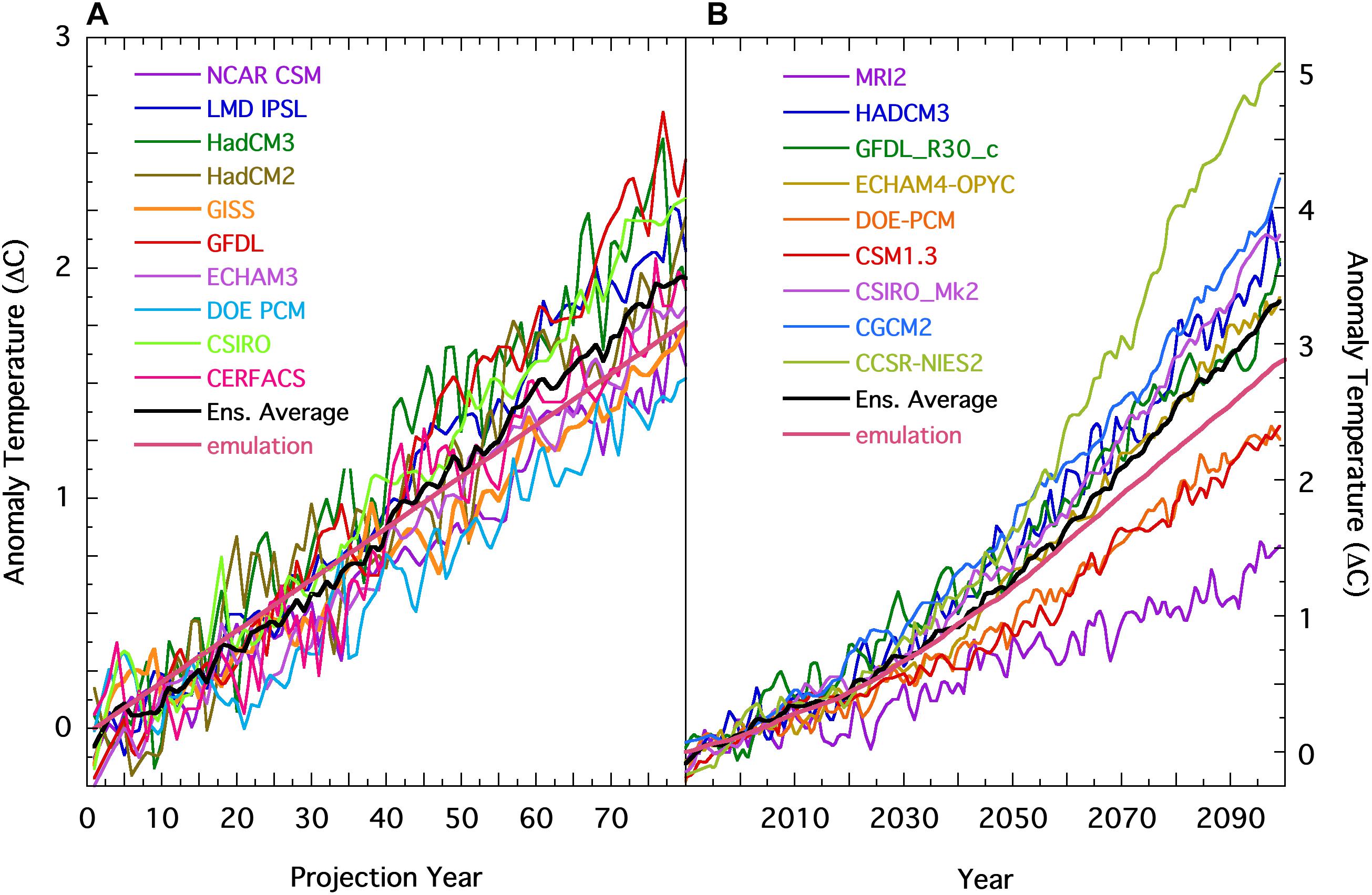
Figure 1. (A) Climate model projections of future GASAT anomalies following a 1% annual growth in atmospheric [CO₂]; (—), the model ensemble average, and; (—), equation 1. Model realizations were obtained from Figure 27 in Covey et al. (2001) (see also Figure 3.10 in AchutaRao et al., 2004). (B) Lines as for part a, showing multiple GCM projections of the SRES A2 scenario from the IPCC. The individual model realizations were obtained from Figure 9.6 in the WG1 Report of the IPCC 3AR (IPCC, 2001). The forcings for the SRES A2 scenario used for the equation 1 emulation were obtained from Appendix II, Table II.3.11 in the WG1 Report (IPCC, 2001). The smooth emulation lines are in the midst of the projection lines.

Figures 1A,B show that equation 1 with f_CO2 = 0.42 produced trends that are well within the envelope of the GASAT projections of fully realized climate models, and is close to the ensemble average in each scenario. The trends produced by equation 1 are also consistent with the general shape of the GCM projections. This consistency indicates that the curvature in projected air temperature is determined by the trend in GHG forcing, as expected for linear dependence. The same fidelity is demonstrated in the emulations of projections from nine GCMs driven by IPCC SRES scenario B2 (see Figure S3-1 in the Supporting Information) (IPCC, 2001).

The Goddard Institute for Space Studies (GISS) Model E GCM was used to determine that water vapor enhanced CO₂ forcing accounts for 20% of the total greenhouse effect (Lacis et al., 2010). However, direct inspection of Figure 1A shows that the parameterizations and climate sensitivity used to make that 20% estimate are representative of GISS Model E only, and are neither necessarily inherent to all climate models nor necessarily generalizable beyond Model E (Knutti and Hegerl, 2008; Lemoine, 2010; Sanderson, 2010). That is, the variation among the projected trends in Figures 1A,B clearly indicates disparate magnitudes of CO₂ climate sensitivity within the several GCMs.

In Figure 1A the temperature trend projected by the GISS model is somewhat below the ensemble average. With all else being equal, and given the 20% of GISS model E, the fractional transient greenhouse forcing due to CO₂ within the GCMs ranges from about 18% (DOE-PCM) to about 30% (GFDL). This illustrates that the sensitivity of the terrestrial climate to greenhouse gas forcing as derived from any one climate model is not generalizable to other models and is thus also not necessarily indicative of the physically real response of the terrestrial climate.

Figure 2 shows the further successful emulations of SRES A2, B1, and A1B GASAT projections made using six different CMIP3 GCMs. In the Supporting Information, Figure S4-1 through Figure S4-5 present 30 additional successful emulations of SRES air temperature projections representing seventeen CMIP3 GCMs. For all the emulations, the values of f_{CO_2} and the coefficient a varied with the climate model. The individual coefficients were again determined for each individual projection from fits to plots of standard forcing versus projection temperature (cf. Section 3.2 of the Supporting Information). The values of f_CO2 and a pertaining to Figure 2 are given in Table S4-1, Table S4-2, and Table S4-3, of the Supporting Information. Projection minus emulation residuals, shown in Figure S4-6 in the Supporting Information, are all very near the zero line. Figure 2 and its difference residuals plus the further SRES emulations of Figures S4-1 through S4-5 in the Supporting Information represent successful emulations of 58 IPCC AR4 SRES projections made using 21 different CMIP3 GCMs.

FIGURE 2

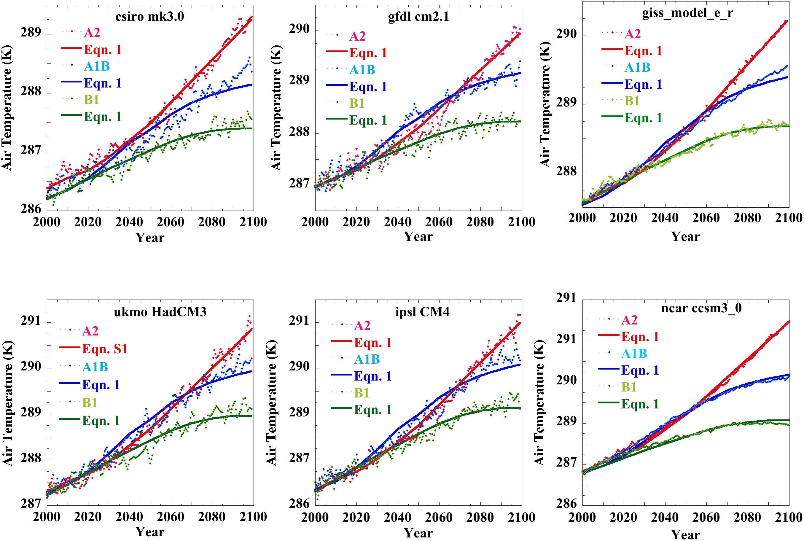
Figure 2. CMIP3 SRES air temperature projections and their equation 1 emulations: (colored points), SRES B1, A1B, and A2 scenario global air temperatures projected by representative CMIP3 GCMs, and; (colored lines), the same scenarios emulated using equation 1. The equation 1 coefficients for the individual emulations are given in Table S4-1, Table S4-2, and Table S4-3 of the Supporting Information. Figure S5-1 shows the emulation coefficients are highly correlated among the tested models (R = 0.98). The 4AR SRES anomalies were obtained from the IPCC electronic source: http://www.ipcc-data.org/data/ar4_multimodel _globalmean_tas.txt. Projection minus emulation difference anomalies may be found in Figure S4-6 in the Supporting Information.

Figures 3A,B above extend the equation 1 emulations to the CMIP 5 GISS-E2-H and BCC-CSM1-1 GCM projections of Representative Concentration Pathway (RCP) scenarios RCP4.5 and RCP8.5, which appeared in the 2013 IPCC 5AR. The CMIP5 RCP simulations were downloaded from the KNMI Climate Explorer website: http://climexp.knmi.nl/selectfield_cmip5.cgi?id=rtisdale@snet.net. The RCP forcings used for the emulations were from Meinshausen et al. (2011), and include solar and 25% volcanic forcing.

FIGURE 3

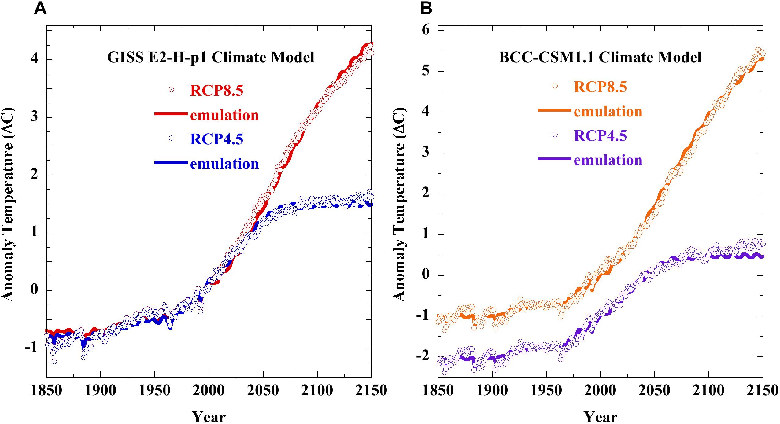
Figure 3. Equation 1 emulation of CMIP5 RCP4.5 and RCP8.5 air temperature projections. Panel (A) (points), the GISS GCM Model-E2-H-p1, and; (lines), the emulations. Panel (B) (points), the Beijing Climate Center Climate System GCM Model 1-1 (BCC-CSM1-1), and; (lines), the emulations. In (B), the vertical offset of RCP4.5 was present in the downloaded data. The equation 1 coefficients were (f_CO2, a; RCP4.5 and RCP8.5): GISS: 0.578 ± 0.004, 20.0 ± 0.1, and; 0.488 ± 0.001, 16.93 ± 0.05; BCC: 0.636 ± 0.004, 23.2 ± 0.1, and; 0.680 ± 0.003, 23.7 ± 0.1, respectively. In (B), the RCP4.5 emulation begins to depart from the GCM projection after 2050, when forcing becomes constant. The GISS and BCM models treat this region differently.

Additionally, emulations of a further thirteen RCP projections made using six different CMIP5 GCMs are shown in Figure S4-7 and Table S4-4 in the Supporting Information. The corresponding projection minus emulation difference residuals are shown in Figure S4-8 in the Supporting Information. These residuals are again very near to the zero line.

Emulations of the 20th century global air temperature record, Figure S9-1 and Figure S9-2 of the Supporting Information, also compare favorably with those of advanced climate models, as shown in Figure S9-3.

The success of equation 1 shows that GCM projections of emissions-driven global air temperature projections are just linear extrapolations of the fractional change in GHG forcing. The variability of emulation coefficients in Table S4-4 also clearly shows that individual GCMs deploy unequal transient climate sensitivities (Kiehl, 2007).

The finding that GCMs project air temperatures as just linear extrapolations of greenhouse gas emissions permits a linear propagation of error through the projection. In linear propagation of error, the uncertainty in a calculated final state is the root-sum-square of the error-derived uncertainties in the calculated intermediate states (see Section 2.4 below) (Taylor and Kuyatt, 1994). Linear propagation of GCM error is appropriate for estimating the uncertainty of the linear extrapolations that are GCM global air temperature projections. Propagation of error is a standard measure of model reliability [(Vasquez and Whiting, 2006), (see also Section 5 in the JCGM Guide) (JCGM, 2008)], and in this case will provide an estimate of the reliability of GCM global air temperature projections.

To that end, the GCM calibration error due to incorrectly simulated cloud cover is described next [see Section CMIP5 Model Calibration Error in Global Average Annual Total Cloud Fraction (TCF)]. Following this, Section “A Lower Limit of Uncertainty in the Modeled Global Average Annual Thermal Energy Flux” will propagate GCM calibration error through their air temperature projections.

CMIP5 Model Calibration Error in Global Average Annual Total Cloud Fraction (TCF)

Scientific instrumentation may be viewed as expressing physical relationships in hardware. Likewise, scientific models running on computers are physical relationships expressed in software. Instrumental resolution is the smallest magnitude the given device can accurately and reliably measure. For a physical model, the resolution limit is the smallest perturbation or physical feature that the model can accurately and reliably simulate. Instrumental accuracy is determined by calibration against external measurement standards (Eisenhart, 1963, 1968). By the same token, model accuracy is determined by a calibration simulation compared against an external standard, often an accurately known observation (Vasquez and Whiting, 1998, 2006; Roy and Oberkampf, 2011). Calibration error can be both systematic and random (Eisenhart, 1963; Ku, 1966). While random error can average away, systematic error does not. Systematic error must be determined empirically because it is typically of unknown magnitude and can vary with the instrument or the model, or with uncontrolled variables (Morrison, 1971; Roy and Oberkampf, 2011). Calibration error conditions the accuracy statements of all subsequent instrumental measurements or model expectation values (Vasquez and Whiting, 2006; JCGM, 2008; Garafolo and Daniels, 2014) (see also Section F 1.2.3ff in the JCGM Guide).

The CMIP5 GCMs implement the known physics of climate and provide the foundation of the 2013 Fifth Assessment Report of the IPCC (5AR). The accuracy of CMIP5-level GCMs has been calibrated by comparison of simulated global cloud fraction and atmospheric water vapor against their observations (Jiang et al., 2012; Klein et al., 2013; Lauer and Hamilton, 2013; Su et al., 2013). The calibrations were particularly penetrating, as they took advantage of high-resolution A-Train satellite observations. These calibration results are now used herein to extract and examine the CMIP5-level total cloud fraction (TCF) error.

CMIP5 global cloud calibration error can be derived by comparing 25-year (1980–2004) GCM annual TCF hindcast cloud simulation means against appropriate A-train observational averages (Jiang et al., 2012). For this comparison, the target global MODIS and ISCCP2 observed total cloud fractions were averaged to produce the mean global TCF. Individual annual average GCM TCF error was then computed as the simple difference between each 25-year annual mean hindcast and the averaged observed TCF field (see Section S6 and Figure S6-1 of the Supporting Information for the sources of the mean simulated and observed TCF).

Figure 4 presents the individual 25-year mean annual global TCF hindcast errors made by 12 CMIP5-level climate models. Any true random error in annual TCF should have been reduced by a factor of 5 in the 25-year hindcast means. However, the error profiles of the GCM cloud fraction means do not display random-like dispersions around the zero-error line. They are all of a similar shape, and the unmistakable similarities strongly support an inference of common systematic origin. This inference is specifically supported by the highly similar errors produced by the two versions of GISS Model E (described further below).

FIGURE 4

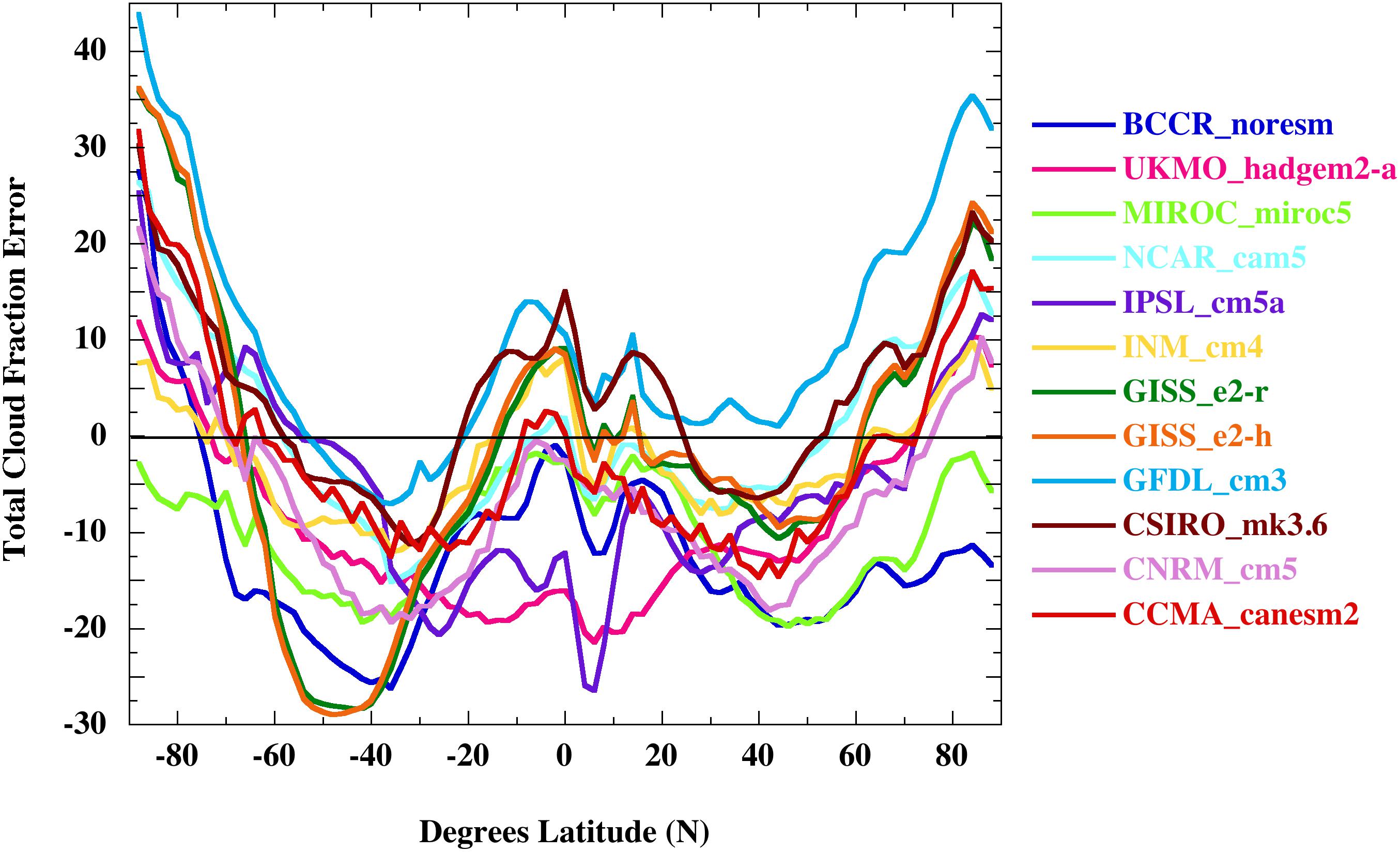
Figure 4. Total 25-year ensemble mean (hindcast minus observed) fractional TCF error (×100) over 1980–2004 of each of the 12 CMIP5-level climate models listed next to the right ordinate. Mean observed cloud fraction was the global 25-year average [(MODIS + ISCCP2)/2] satellite TCF observations. See Section S6 and Figure S6-1 of the Supporting Information for further details.

Although not discussed further here, the CMIP3 models produced very similar TCF error residuals (Jiang et al., 2012). Direct inspection of Figure 4 is enough to show that the sign of the TCF error is variable.

The Structure of CMIP5 TCF Error

The CMIP5 hindcast error residuals of Figure 4 were first assessed for lag-1 autocorrelation. For a data series, x₁, x₂,…, x_n, a test for lag-1 autocorrelation plots every point x_i against point x_i+1. A large autocorrelation R-value means the magnitudes of the x_i+1 are closely descended from the magnitudes of the x_i. For a smoothly deterministic theory, extensive autocorrelation of an ensemble mean error residual shows that the error includes some systematic part of the observable. That is, it shows the simulation is incomplete. Figure 5 shows this test applied to the annual average TCF hindcast error of the CSIRO_mk3.6 climate model.

FIGURE 5

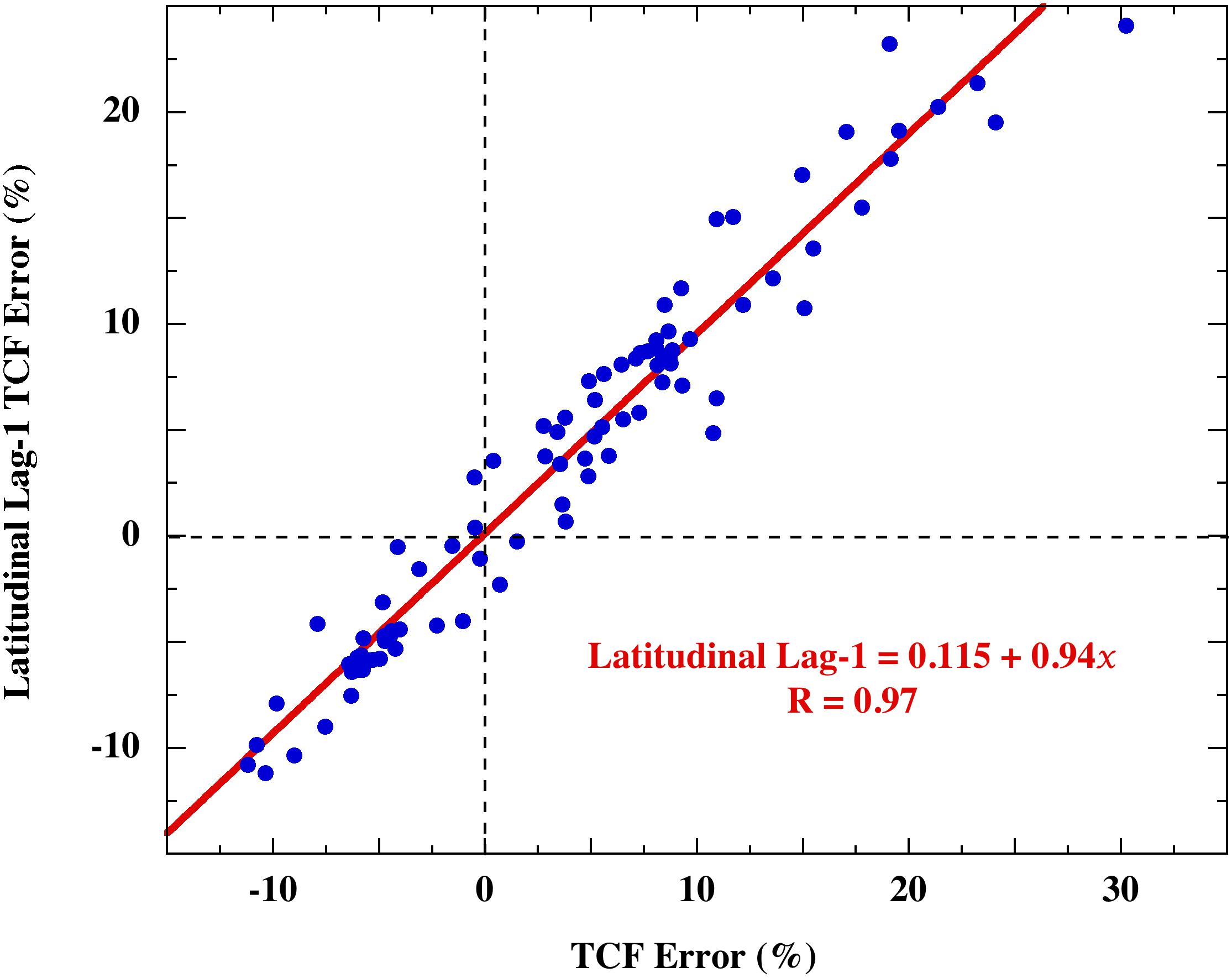
Figure 5. Points: the lag-1 autocorrelation of the CSIRO_mk3.6 climate model average annual TCF hindcast (observed minus simulated) error residual that appeared in Figure 4. The line is a linear least squares fit.

The highly autocorrelated lag-1 error (R = 0.97) implies that systematic cloud effects remain in the error residual. This in turn indicates that the CSIRO GCM systematically misrepresented the terrestrial cloud cover.

Table 1 shows that the high CSIRO_mk3.6 climate model lag-1 autocorrelation of error is typical of every tested CMIP5 climate model. All of the models produced TCF error residuals of lag-1 autocorrelation R ≥ 0.95, and incorrectly simulated the terrestrial cloud cover.

TABLE 1

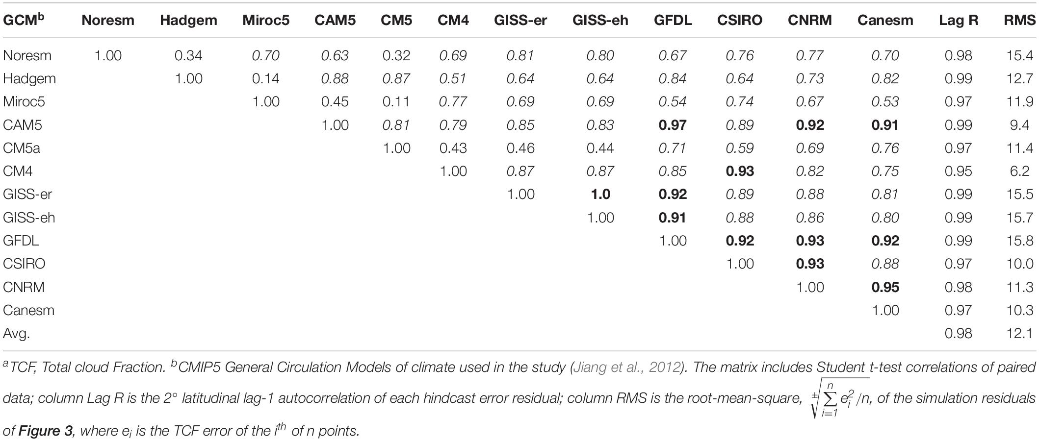
Table 1. Student-t correlation matrix, Lag-1 R values, and RMS uncertainty of CMIP5 Model TCF^a error residuals.

If the model annual TCF errors were random, then cloud error would disappear in multi-year averages. Likewise, the lag-1 autocorrelation of error would be small or absent in a 25-year mean. However, the uniformly strong lag-1 autocorrelations and the similarity of the error profiles (Figure 4 and Table 1) demonstrate that CMIP5 GCM TCF errors are deterministic, not random. The autocorrelation is unlikely to reflect random persistence because every tested TCF is a 25-year hindcast mean.

The structure of TCF error among the models was further examined by evaluating inter-model pair-wise correlations. If the TCF errors independently produced by two models are highly correlated, then evidence is adduced that the models deploy theoretical structures that share mistakes in common. Thus, pair-wise correlations were assessed across all the GCM TCF error residuals, producing 66 unique comparisons (Table 1). Of these, twelve error pairs exhibited correlation R ≥ 0.9 (highlighted in bold). Thirty-eight pairs produced correlations 0.9 > R ≥ 0.5 (in italics).

For a population of white noise random-value series with normally distributed pair-wise correlations, the most probable pair-wise correlation is zero. If the TCF errors were thus random, the probability that any two error-series would exhibit a correlation R = 0.9 is about 10^–17. Likewise, a pair-wise correlation R = 0.5 would occur at a rate of approximately 10^–5. The multiple high-positive pair-wise correlations therefore indicate that the CMIP5 TCF simulation errors are not random but instead imply a common systematic cause. The most likely common cause is a widely shared error in the implemented theory (Stainforth et al., 2007; Pennell and Reichler, 2010). In an analogous surmise, the average positive correlation of CMIP3 model inaccuracies in simulated GASAT has likewise been taken to imply systematic errors in theory (Knutti et al., 2010).

The terrestrial climate can exhibit chaotic behavior (Heagy et al., 1994; Dymnikov and Gritsoun, 2001; Shao, 2002; Rial, 2004). Physical chaos can be described as, “aperiodic long-term behavior in a deterministic (physical) system that exhibits sensitive dependence on initial conditions” (Wagner, 2011). A single instance of deviation between a model realization and observations due to chaos-driven GCM internal variability might be impossible to distinguish from the systematic error following from an erroneous or incomplete theory (Sugihara and May, 1990). Were the ±12% deviations in simulated TCF discussed above due to chaos-driven internal variability of the models, their global air temperature projections should be strongly impacted because TCF directly impacts tropospheric thermal energy flux (see Section 2.3 below). Model internal variability is the chief source of noise evident in air temperature projections (Dessler et al., 2018; Adams and Dessler, 2019). However, large-scale deviations from the observed global air temperature target are manifestly not present in global air temperature hindcasts (Dessler et al., 2018) [(IPCC, 2013) cf. Figure TS 9, TFE3 Figure 1, 9.8, Box 10.1 Figure 1, 10.1)]. The coherence of GCM hindcasts with observations is sufficient to exclude chaotic behavior as the origin of the TCF deviations shown in Figure 4.

The conclusion that TCF calibration error derives from systematic errors in the physical theory is strengthened on noting that the two versions of the GISS model produced the most highly correlated TCF lag-1 error (R = 1.0). The two Model E versions share a common origin and among the models undoubtedly share the greatest similarity in elaborated theory and parameterizations (Stainforth et al., 2007). Were cloud simulation errors invariably random, those models deploying a similar physical core and a similar parameter set should nevertheless produce errors no more inter-correlated than comparisons with the random errors of other models with alternative physical cores. That the structurally most similar models produce the most highly correlated error demonstrates internal model theory-error as the source of the systematic inaccuracies in cloud simulations.

A similar pair-wise analysis of AMIP1-level model global TCF error residuals produced notably weaker inter-model correlations (Frank, 2008). Among forty-six AMIP1 comparisons, only four yielded correlation R ≥ 0.9 and thirteen 0.9 > |R| ≥ 0.5. The average AMIP1 RMS global cloud error was ±10.1%, relative to their ISCCP1 target. The stronger correlations among the CMIP5 hindcast error residuals, along with their average ±12.1% RMS error, imply a convergence of theoretical structure since 1999 without an improvement in TCF verisimilitude.

A Lower Limit of Uncertainty in the Modeled Global Average Annual Thermal Energy Flux

The Magnitude of CMIP5 TCF Global Average Atmospheric Thermal Energy Flux Error

Lauer and Hamilton (2013) have quantified CMIP3 and CMIP5 TCF model calibration error in terms of cloud forcings. They compared the average of observed cloud properties with a 20-year (1986–2005) annual mean simulation hindcast. CMIP model error was derived as the differences in modeled (x^mod) and observed (x^obs) 20-year means. The mean bias for N models was defined as,

${\mathrm{\Delta }}^{mm}=\frac{1}{N}\sum _{i=1}^N(x_i^{\text{mod}}-x^{obs})(2)$

In equation 2, x_i^mod is 20-year simulation cloud cover mean over each of the global grid-points for each model, and the x^obs is the corresponding observational mean at that grid-point. This difference is a CMIP model calibration error referenced to the observational standard. The derivational logic following from equation 2 is presented in Section S6.2 of the Supporting Information.

Dimensional analysis of the derivation yields the units of the calibration error statistic: Σ_{20 years}($x_i^{\text{mod}}-x^{obs}$) × 1/20 years = ($x_i^{\text{mod}}-x^{obs}$) year^–1. Figure 4 shows that individual annual mean grid-point $x_i^{\text{mod}}-x^{obs}$ errors can be of positive or negative sign. The global annual mean simulation uncertainty in cloud cover for any CMIP model is the root-mean-square (RMS) of the global array of the 20-year grid-point ($x_i^{\text{mod}}-x^{obs}$) annual model error means (see Section S6.2 in the Supporting Information for details).

For “N” CMIP GCMs, the ensemble average errors are combined as the RMS. This process yields the GCM average calibration error statistic in simulated cloud cover. That error is of dimension ± (cloud-cover-unit) year^–1. This calibration error statistic is the average annual uncertainty in simulated cloud cover across any given projection year to be expected for a representative set of CMIP models.

The annual mean CMIP uncertainty in global annual cloud cover, ±(cloud-cover-unit) year^–1, must be converted into the uncertainty in annual mean CMIP long-wave cloud forcing (LWCF) in units of ±Wm^–2. This yields the uncertainty in tropospheric thermal energy flux, i.e., ±(cloud-cover-unit) × [Wm^–2/(cloud-cover-unit)] = ± Wm^–2 year^–1. It is assumed here that the CMIP5 LWCF error is also a lower limit of error for all climate models of earlier CMIP vintage.

Global cloud forcing (CF) is net cooling, with an estimated global average annual magnitude of about −27.6 Wm^–2 (Hartmann et al., 1992; Stephens, 2005). The average ±12.1% RMS error in TCF made by the CMIP5 climate models implies that CF is incorrectly simulated. Lauer and Hamilton divided CF into short-wave cloud forcing (SCF) and long wave cloud forcing (LWCF) exerted at the top of the atmosphere (TOA), representing reflected radiant energy and long-wave radiant energy propagating upward from the surface, respectively (Lauer and Hamilton, 2013). LWCF represents the contribution made by clouds to the thermal radiation flux of the atmosphere.

On conversion of the above CMIP cloud root-mean-squared error (RMSE) as ±(cloud-cover unit) year^–1 model^–1 into a longwave cloud-forcing uncertainty statistic, the global LWCF calibration RMSE becomes ±Wm^–2 year^–1 model^–1 The CMIP5 models were reported to produce an annual average LWCF RMSE = ± 4 Wm^–2 year^–1 model^–1, relative to the observational cloud standard (Lauer and Hamilton, 2013). This calibration error represents the average annual uncertainty within any CMIP5 simulated tropospheric thermal energy flux and is generally representative of all CMIP5 models.

By way of comparison, the CMIP5 long wave cloud forcing error reported for 10 GCMs in Figure 6 of Zhang et al. (2005), and for 28 GCMs in Figure 3 of Dolinar et al. (2015) were evaluated (Zhang et al., 2005; Dolinar et al., 2015). The RMS error in simulated long wave cloud forcing were estimated to be ±4.9 Wm^–2 and ±4.5 Wm^–2, respectively. Alternatively, the average CERES/ERBE/ISCCP long wave cloud radiative forcing reported in Zhang et al. (2005) and in Dolinar et al. (2015), are 28.2 Wm^–2 and 27.6 Wm^–2, respectively. If the ±12.1% CMIP5 cloud simulation error originally reported in Jiang et al. (2012) is assumed to be uniformly distributed among all cloud types, then simulated long wave cloud error can be estimated from the observed LWCF to be ±3.4 Wm^–2 or ±3.3 Wm^–2 (Jiang et al., 2012). These four values are comparable to and bracket the ±4 Wm^–2 employed in this study (Lauer and Hamilton, 2013).

FIGURE 6

Figure 6. Panel (A), SRES scenarios from IPCC 4AR WGI Figure SPM.5 (IPCC, 2007), with uncertainty bars representing, “the±1 standard deviation range of individual model annual averages.” Panel (B) the identical SRES scenarios showing the ±1σ uncertainty bars due to the annual average ±4 Wm^–2 CMIP5 TCF long-wave tropospheric thermal flux calibration error propagated in annual steps through the projections as equation 5 and equation 6.

CMIP5 error in LWCF implies that the magnitude of the thermal energy flux within the atmosphere is simulated incorrectly. This climate model error represents a range of atmospheric energy flux uncertainty within which smaller energetic effects cannot be resolved within any CMIP5 simulation. Thus, the LWCF calibration error of ±4 Wm^–2 year^–1 is an average CMIP5 lower limit of resolution for atmospheric forcing. This means the uncertainty in simulated LWCF defines a lower limit of ignorance concerning the annual average thermal energy flux in a simulated troposphere (cf. Supporting Information Section 10.2).

GHG forcing enters into and is not separable from the total flux of thermal energy within the troposphere (Berger and Tricot, 1992; IPCC, 2013); cf. Figure 7.1 in IPCC, 2013. Therefore, model simulations of the climatic response to changes in GHG atmospheric forcing are conditioned by ±4 Wm^–2 of uncertainty in the magnitude of thermal energy flux within the troposphere. In short, CMIP5 climate models are unable to reliably simulate, determine, or bring into view the effect of a tropospheric thermal flux perturbation of magnitude within the ±4 Wm^–2 bound. That is, the ±4 Wm^–2 calibration error constitutes a lower limit of model resolution.

Bringing this idea into context, this annual average ±4.0 Wm^–2 year^–1 uncertainty in simulated LWCF is approximately ±150% larger than all the forcing due to all the anthropogenic greenhouse gases put into the atmosphere since 1900 (∼2.6 Wm^–2). Further, the ±4.0 Wm^–2 year^–1 LWCF error is approximately ±114 × larger than the average annual ∼0.035 Wm^–2 year^–1 increase in greenhouse gas forcing since 1979 (Hofmann et al., 2006; IPCC, 2013).

Linear Models and Error Propagation

To this point, GCM air temperature projections have been demonstrated to be linear extrapolations of greenhouse gas forcing. The reliability of these projections must be conditioned by the impact of the uncertainty in simulated tropospheric thermal energy flux. To that end, error propagation is introduced.

Propagation of error is a standard method used to estimate the uncertainty of a prediction, i.e., its reliability, when the physically true value of the predictand is unknown (Bevington and Robinson, 2003). For example, in a single calculation of x = f(u,v,…), where u, v, etc., are measured magnitudes with uncertainties in accuracy of ±(σ_u,σ_v,…), then the uncertainty variance propagated into x is,

${\mathrm{\sigma }}_x^2={\mathrm{\sigma }}_u^2{(\frac{\delta x}{\delta u})}^2+{\mathrm{\sigma }}_v^2(\frac{\delta x}{\delta v})+\mathrm{\dots }+2{\mathrm{\sigma }}_{u,v}^2(\frac{\delta x}{\delta u})(\frac{\delta x}{\delta u})+\mathrm{\dots }(3)$

Likewise, if a final state, X_N, is calculated through a serial progression of prior states, i.e., X_N = f(x₀,…,x_i,…,x_n), where the x_i are intermediate states, then a serial propagation of physical error through n steps yields the uncertainty variance in the realization of the final state,

${\text{σ}}_{X_N}^2={\text{σ}}_i^2{(\frac{\delta X_N}{\delta x_i})}^2+{\text{σ}}_{i+1}^2{(\frac{\delta X_N}{\delta x_{i+1}})}^2+\mathrm{...}+2{\text{σ}}_{i,i+1}^2(\frac{\delta X_N}{\delta x_i})(\frac{\delta X_N}{\delta x_{i+1}})+\mathrm{...}(i = 0,\mathrm{...},n)(4)$

That is, a measure of the predictive reliability of the final state obtained by a sequentially calculated progression of precursor states is found by serially propagating known physical errors through the individual steps into the predicted final state. When states x_0,., x_n represent a time-evolving system, then the model expectation value X_N is a prediction of a future state and ${\mathrm{\sigma }}_{X_N}^2$ is a measure of the confidence to be invested in that prediction, i.e., its reliability. Propagation equation 4 is directly relevant to evaluating the impact of systematic calibration error on the reliability of complex physical models (Vasquez and Whiting, 1998, 2006). The ISO JCGM “Guide to the Expression of Uncertainty” likewise recommends propagation of systematic error as the root-sum square (JCGM, 2008, cf. Sections 5.1.3–5.1.5).

Applying these concepts, air temperature projections involve a step-wise sum of model realizations of serial future climate states (x₀…x_n) through to some final climate state, X_N (Pope et al., 2000; Saitoh and Wakashima, 2000; IPCC, 2007, 2013). Each intermediate climate state in the series provides the initial conditions for a simulation of the subsequent state. These step-wise simulated states are subject to propagation of error as described above and in equation 4.

The final change in projected air temperature is just a linear sum of the linear projections of intermediate temperature changes. Following from equation 4, the uncertainty “u” in a sum is just the root-sum-square of the uncertainties in the variables summed together, i.e., for c = a + b + d + … + z, then the uncertainty in c is $\pm u_c=\sqrt{u_a^2+u_b^2+u_d^2+\mathrm{\dots }+u_z^2}$ (Bevington and Robinson, 2003). The linearity that completely describes air temperature projections justifies the linear propagation of error. Thus, the uncertainty in a final projected air temperature is the root-sum-square of the uncertainties in the summed intermediate air temperatures.

The errors made by GCMs in simulating cloud cover produce errors in the simulated tropospheric thermal energy flux (Hartmann et al., 1992; Chen et al., 2000; Bony and Dufresne, 2005; Stephens, 2005; Turner et al., 2007; Bony et al., 2011). The error in the intensity of simulated tropospheric thermal energy flux in turn injects errors into projected air temperature. Nevertheless, propagation of error is remarkable by its absence in any discussions of uncertainty in climate prediction (Collins, 2007; Stainforth et al., 2007; Curry, 2011; Curry and Webster, 2011; Hegerl et al., 2011).

Introducing CMIP LWCF Error Into Emulation Equation 1

Figures 1–3, as well as Figures 7, 8 below and Supporting InformationFigures S3-1, S4-1 through S4-6, and Figure S8-1 demonstrate that equation 1 successfully emulates the air temperature projections of advanced climate models, including the CMIP5 versions. Equation 1 indicates that advanced GCMs simulate the impact of tropospheric thermal forcing on air temperature as linear extrapolations of fractional greenhouse gas forcing.

FIGURE 7

Figure 7. Panel (A) (points), the CMIP5 multi-model mean anomaly projections of the 5AR RCP4.5 (o, 21 models) and RCP8.5 (o, 21 models); (full lines), the equation 1 emulations of the CMIP5 mean projections. The standard RCP forcings including solar and 25% volcanic forcing were used throughout (Meinshausen et al., 2011). Individual CMIP5 mean forcings may not be identical to the Meinhausen RCP forcings. Panel (B): (colored lines), the same two CMIP5 mean RCP projections with uncertainty envelopes derived from propagating the annual average ± 4 Wm^–2 CMIP5 long wave cloud forcing error as in equations 5 and equation 6, starting from projection year 2005. For RCP4.5, the emulation departs from the mean near projection year 2050 when GHG forcing becomes constant.

FIGURE 8

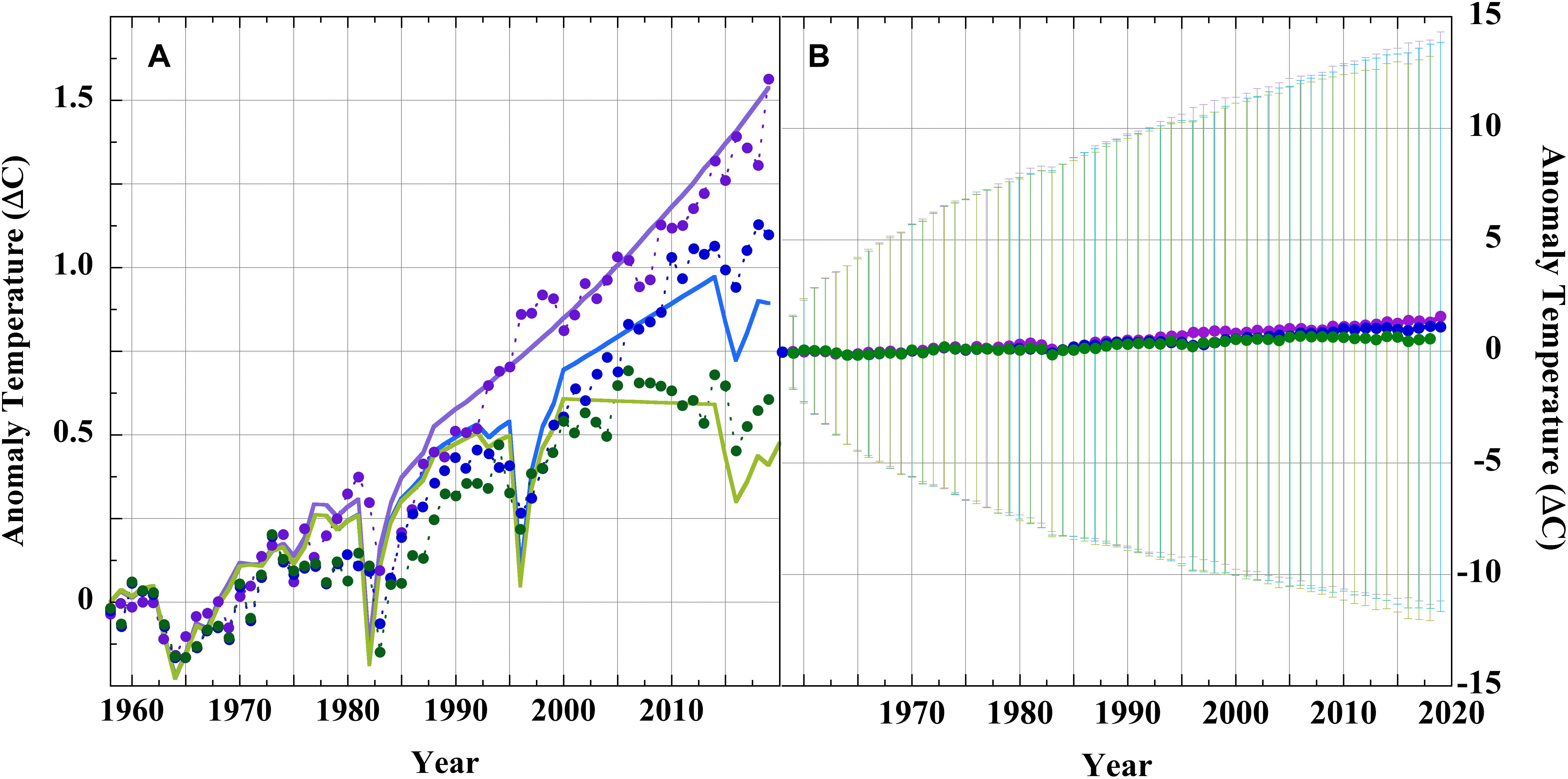
Figure 8. Panel (A): (points), historical air temperature projections of GISS Model II GCM for; (∙), scenario A; (∙), scenario B, and; (∙), scenario C (Hansen et al., 1988; Schmidt, 2007a, b). (Lines), equation 1 emulation of: (—), scenario A; (—), scenario B, and; (—), scenario C, with Y₀ = 1958, T_GHG(1958) = 33.25 K, f_CO2 = 0.42, F₀ = 33.946 Wm^–2 (CO₂, N₂O, and CH₄ forcing only). Panel (B): The same A, B, and C scenario projections but with uncertainty bars from ±4 Wm^–2 CMIP5-level LWCF calibration error propagated as equation 6.

GHG forcing enters into and becomes part of the global tropospheric thermal flux. Therefore, any uncertainty in simulated global tropospheric thermal flux, such as LWCF error, must condition the resolution limit of any simulated thermal effect arising from changes in GHG forcing, including global air temperature. LWCF calibration error can thus be combined with ΔF_i in equation 1 to estimate the impact of the uncertainty in tropospheric thermal energy flux on the reliability of projected global air temperatures.

To be kept in mind during this exercise is that the source of calibration error is inherent within the physical theory deployed by CMIP GCMs. This means that the error in LWCF arises in the GCM and enters into every step of a simulation. Each step includes a fresh simulation of cloud cover; and each fresh simulation will include a LWCF thermal flux error. An inherently incorrect theory puts its intrinsic error into every simulation step. This point is critical and is discussed further below.

The CMIP5 average annual LWCF ± 4.0 Wm^–2 year^–1 calibration thermal flux error is now combined with the thermal flux due to GHG emissions in emulation equation 1, to produce equation 5. This will provide an estimate of the uncertainty in any tropospheric global air temperature projection made using a CMIP5 GCM. In equation 5 the step-wise GHG forcing term, ΔF_i, is conditioned by the uncertainty in thermal flux in every step due to the continual imposition of LWCF thermal flux calibration error.

$\mathrm{\Delta }{T}_i(K)\pm u_i=0.42\times 33K\times [(F_0+\mathrm{\Delta }{F}_i\pm 4W{m}^2)/F_0](5.1)$

and

$\Delta T_i(K)\pm u_i=0.42\times 33K\times [(F_0+\Delta F_i)/F_0]\pm [0.42\times 33K\times 4W{m}^2/F_0](5.2)$

Where ±u_i is the uncertainty in air temperature, and ±4 Wm^–2 is the uncertainty in tropospheric thermal energy flux due to CMIP5 LWCF calibration error. The remaining terms of equations 5 are defined as for equation 1. In equations 5, F₀ + ΔF_i represents the tropospheric GHG thermal forcing at simulation step “i.” The thermal impact of F₀ + ΔF_i is conditioned by the uncertainty in atmospheric thermal energy flux. That is, resolution of GHG forcing is subject to the uncertainty in simulated tropospheric thermal energy flux due to LWCF model thermal flux calibration error.

The rationale for equations 5 is straightforward. The response of the physical climate to increased CO₂ forcing includes the response of global cloud cover. However, global average cloud cover is not simulated to better than ±12.1%. The error in simulated cloud cover in turn produces an error in the thermal energy flux of the simulated troposphere. The impact of a 0.035 Wm^–2 annual forcing change on cloud cover due to increased CO₂ cannot be resolved, or simulated by, climate models that have a ±4 Wm^–2 resolution lower limit. Nor can the models resolve the subsequent feedback response of cloud cover to the very small increase in tropospheric thermal energy flux due to CO₂ forcing. Thus, neither the outcome of the forcing nor the feedback response can be resolved. In short, the ±4 Wm^–2 LWCF uncertainty specifically conditions ΔF_i because CO₂ forcing enters into the total tropospheric thermal energy flux and becomes part of it.

This should be seen in light of the fact that the mean annual thermal perturbation to tropospheric thermal energy flux due to GHG emissions is less than 1% of the uncertainty in tropospheric thermal energy flux due to LWCF error, alone. Following from equation 4, the final uncertainty envelope about a multi-year projection is the ±u_i of equations 5 propagated through the emulation as the root-sum-square (see 2.4.3 below) (Vasquez and Whiting, 2006; JCGM, 2008; Garafolo and Daniels, 2014).

Error Propagation and the Uncertainty in Projected GASATs

Projections of future air temperatures proceed in discrete time-steps (Pope et al., 2000; Saitoh and Wakashima, 2000) (cf. also Box 9.1 and Box 11.1 in WG1 of the IPCC 5AR) (IPCC, 2013). In a climate projection of “n” steps, each time step “i” initializes with the climate variables delivered by the “i-1” step. Air temperature follows from the total flux of thermal energy through the atmosphere. The expression for uncertainty described next follows the guidelines in Section 5 of, “The Guide to the Expression of Uncertainty in Measurement” (JCGM, 2008), and descends directly from equation 3, equation 4, and equations 5, and Section “CMIP5 Model Calibration Error in Global Average Annual Total Cloud Fraction (TCF)” through Section “Linear Models and Error Propagation.” The approach also follows the recommendations for evaluating systematic errors in numerical models (cf. equation 2 in Vasquez and Whiting, 2006).

Vasquez and Whiting (2006) also point out that even random error does not diminish as 1/√N in non-linear models, because the non-linearity produces skewed distributions of expectation values. However, this extended error is not evaluated here.

For the uncertainty analysis below, the emulated air temperature projections were calculated in annual time steps using equation 1, with the conditions of year 1900 as the reference state (see above). The annual average CMIP5 LWCF calibration uncertainty, ±4 Wm^–2 year^–1, has the appropriate dimension to condition a projected air temperature emulated in annual time-steps. Following from equations 5, the uncertainty in projected air temperature “T” after “n” projection steps is (Vasquez and Whiting, 2006),

$\pm {\mathrm{\sigma }}_{T_n}=\sqrt{{\sum }_{i=1}^n{[\pm u_i(T)]}^2}(6)$

Equation 6 shows that projection uncertainty must increase with every simulation step, as is expected from the impact of a systematic error in the deployed theory.

Figure 6A shows global air temperature projections for four standard multi-model global means of the IPCC Fourth Assessment Report (4AR) Special Report on Emissions Scenarios (SRES). The uncertainty bars in Figure 6A are taken from the 4AR WG1 Figure SPM.5 and represent “the±1 standard deviation range of individual model annual averages,” i.e., the variation about the means of the multi-model temperature projections. Figure 6B presents the uncertainty for the same SRES projections upon propagating ±4 Wm^–2 of LWCF error, calculated according to equations 5 and equation 6. The SRES temperature anomalies and forcings were obtained from the IPCC 4AR (IPCC, 2007).

The difference between the two representations of uncertainty in Figures 6A,B lays in the fact that in Figure 6A, the uncertainty bars are a statistical measure of inter-model precision. In Figure 6B, the uncertainty bars reflect physical accuracy, and are a statistical measure of projection reliability.

Figure 7 extends this analysis to the CMIP5 air temperature projections of the RCPs appearing in the 2013 IPCC 5AR. Figure 7A presents an equation 1 emulation of multi-model CMIP5 mean projections of the RCP4.5 and RCP8.5 scenarios. For these emulations, the equation 1 parameters were: RCP4.5, f_CO2 = 0.593 ± 0.004, a = 20.4 ± 0.1 and RCP8.5, f_CO2 = 0.585 ± 0.002, and a = 20.19 ± 0.08. Figure S4-7 and Table S4-4 in the Supporting Information show the successful emulations of thirteen additional RCP projections from six CMIP5 GCMs. These successful emulations generalize the uncertainty limits illustrated above to all CMIP5 air temperature projections.

Figure 7B displays the effect of LWCF error propagated through the CMIP5 mean RCP projections of Figure 7A. The uncertainty envelopes again represent the physically real ±4 Wm^–2 annual average LWCF thermal flux calibration error of the CMIP5 models and are a measure of confidence to be placed in the projections. The growth of uncertainty shown in Figures 6B, 7B convey the increasing level of ignorance about the successive physical states of the evolving climate. Ignorance increases because the projection trajectory of the erroneously simulated climate, relative to the future evolution of the physically real climate, cannot be known. This ignorance increases with every simulation time-step.

Figures 6B, 7B show that the uncertainty in projected GASAT is immediately so large that even the first projection year conveys no predictive confidence. This can be understood as following directly from the fact that the annual uncertainty in atmospheric thermal energy flux due to the average annual model LWCF CMIP5 calibration error is ∼ ± 114 × larger than the annual average increase in GHG forcing. That is, the finest resolution of the model is ±114 times larger than the perturbation to be resolved. Consequently, the effect of the perturbation is lost within the very wide uncertainty of the simulation.

The message of the uncertainty envelopes in Figures 6B, 7B is clear: neither the SRES nor the RCP projection scenarios convey reliable information about possible future air temperatures. Further, the realizations are not predictively unique. Each SRES or RCP scenario is fully embedded in the uncertainty spread of all the other scenarios. Individual SRES or RCP projections would not be observationally distinguishable on any time scale, nor would be the fidelity of one or the other scenario relative to any observed temperature trend. These points are discussed further below.

Differencing From a Base-State Climate Does Not Remove Systematic Error

It may be supposed that all model errors are already present in an equilibrated 1850 base-state climate simulation and can be removed from subsequent projected climate states by differencing. However, elimination of model error by differencing has never been empirically validated, and indeed cannot be tested against an 1850 climate that is nearly an observational unknown. Further, this method of eliminating model error is unmentioned in the 2013 IPCC 5th Assessment Report (IPCC, 2013; Stocker et al., 2013).

Nevertheless, it is worthwhile to show that differencing does not remove systematic theory-error. The terrestrial climate is simulated through time as state magnitudes, not as anomalies. The erroneous theory deployed within GCMs, fully illustrated by TCF error, means that an initial physical climate state produced by equilibrium spin-up will be wrong, even if the initial conditions were perfectly known. Further, the magnitudes of the base-state errors will be unknown. This initial-state error follows from an imperfect theory and is not due to the stochasticity of climate stemming from physical chaos.

Theory-error means the available energy is incorrectly partitioned among the internal climate sub-states. A model can be in perfect external energy balance at the TOA all the while still expressing a climate with an internally incorrect energy-state.

The initial equilibrium spin-up climate state is then not a physically correct representation of its energy-state. The error relative to the physically real climate is consequent to this internal model error. The continuing impact of theory-error during a step-wise simulation, means that the erroneous flux magnitudes of the initial spin-up state are again and further incorrectly partitioned within each subsequent climate state. That is, the incorrect structures of the base-state climate, C₀, will themselves be incorrectly projected into and through the subsequent simulation state.

This situation is graphically illustrated in Scheme 1. Following from an initially erroneous C₀ state, systematic theory-error ensures that the newly simulated subsequent climate state, C₁, will suffer further distortions, but of unknown magnitude. State C₁ represents a proposed climate existing at some future time, where physical simulation error cannot be determined. Therefore, it cannot be known that differencing removes error when that error is of unknown magnitude.

SCHEME 1

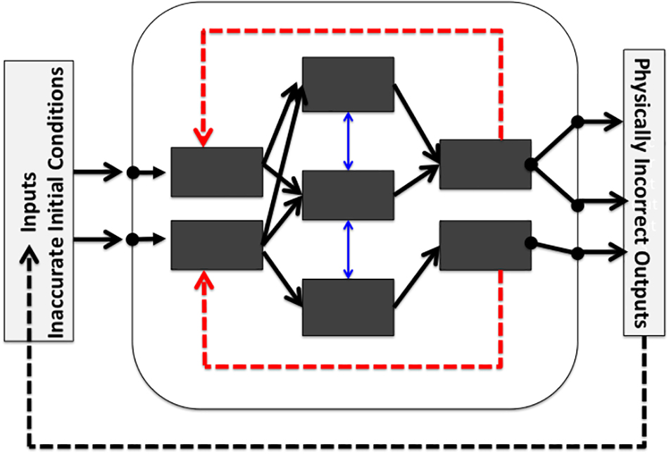
Scheme 1. A stylized representation of a GCM simulation adapted from Fildes and Kourentzes (2011), with permission from Elsevier. Known initial conditions include errors and uncertainties, while others are incompletely known. The inner blue double-headed arrows represent sub-state couplings. The inner red dashed arrows represent internal feedbacks. The external black dashed arrow represents the step-wise simulation circumstance that climate state C_i provides the initial conditions for climate state C_i+1. Thus, errors in state C_i are propagated into state C_i+1. Theory-error means that C_i and C_i+1 are each simulated incorrectly. The errors introduced by C_i are further and incorrectly propagated within the model when simulating C_i+1. This sequence builds error upon error. Theory-error also means that even if the first set of initial conditions were perfectly known, base-state climate C₀ would nevertheless be simulated incorrectly. Model spin-up equilibrates C₀ to an erroneous stable state. The errors in simulated state C₀ are not known to subtract away in calculating climate change because the errors in simulated future climate state C₁ are not known to be identical to those in C₀ (see Section 7.1 in the Supporting Information for an extended discussion).

This circumstance is also implied by the large multiple of simulated climate states produced by models subjected to perturbed physics tests (Rowlands et al., 2012). As Figure 4 shows with TCF calibration error, systematic GCM error persists through high-multiple ensemble means (Annan and Hargreaves, 2004; Palmer et al., 2005; Collins, 2007; Tebaldi and Knutti, 2007).

Supporting Information Section 7, “Differencing and Systematic Theory-bias Model Error” includes a more detailed discussion of simulation differencing. Supporting Information Sections 7.1 “The problem of observational error” and 7.1.1 “The problem of validating a model difference,” address the unresolved problem of differencing using the standard 1850 base-state reference climate (cf. Supporting Information Table S7-1 and text).

A Contemporary Example of Predictive Reliability

A recent analysis proposed statistical measures to suggest that the 1988 scenario B of the GISS Model II GCM included a skillful prediction of the subsequent trend in global averaged air temperatures (Hargreaves, 2010). Figure 8 shows a test of this suggestion in terms of propagated CMIP5 LWCF calibration thermal energy flux error. Figure 8A shows the original Model II A, B, and C scenarios (Hansen et al., 1988). The lines in Figure 8A were calculated using equation 1 and the original scenario forcings (Hansen et al., 1988; Schmidt, 2007a, b). Equation 1 again successfully emulated the projections. Further details of this emulation are given in Section S8 and Figure S8-1 of the Supporting Information.

Figure 8B shows the same 1988 GISS Model II GCM anomaly scenarios A, B, and C, but now including uncertainty bars after propagating the CMIP5-level ± 4 Wm^–2 LWCF calibration error through the projections. The large overlapping uncertainty bars show that projections A, B, and C are not unique. None of them can be validated against observations because the uncertainty envelopes are far larger than any conceivable increase in GASAT. Further, each projection is so deeply embedded in the uncertainties of the alternative projections that it cannot be distinguished by any comparison with observables. For example, in the 1988 GASAT projection year, the scenario anomalies are: A, 0.45 ± 8.9 C; B, 0.36 ± 8.9 C, and; C, 0.25 ± 8.9 C. These are not predictions in any useful or skillful sense. Any statistical similarity between scenario B and the observed subsequent temperature trend is indistinguishable from calculational happenstance and thus is without any physical meaning, a diagnosis also advanced by the original author (Hansen, 2005).

In conjunction with the other equation 1 emulations presented here, Figure 8A also shows that the linear dependence of projected GASAT on fractional GHG forcing has remained a central feature of GCMs for at least 30 years.

Following from this analysis, the uncertainty due to physical LWCF calibration error alone defeats any measure of GCM statistical merit, and is enough to vitiate both the predictive validity of the 1988 GISS Model II GCM scenarios and of all subsequent projections of the GASAT made using GCMs up to and including the present CMIP5 generation.

Conclusion

This analysis has shown that the air temperature projections of advanced climate models are just linear extrapolations of fractional GHG forcing. Linear propagation of model error follows directly from GCM linear extrapolation of forcing. The ±4 Wm^–2 year^–1 annual average LWCF thermal flux error means that the physical theory within climate models incorrectly partitions energy among the internal sub-states of the terrestrial climate. Specifically, GCMs do not capture the physical behavior of terrestrial clouds or, more widely, of the hydrological cycle (Stevens and Bony, 2013). As noted above, a GCM simulation can be in perfect external energy balance at the TOA while still expressing an incorrect internal climate energy-state.

The further meaning of uncertainty in projected air temperature is extensively discussed in Section 10.1 of the Supporting Information, “Why confidence intervals do not imply model oscillation.” Sections 10.2 and 10.3 of the Supporting Information provide an extended discussion of the meaning of confidence intervals, uncertainty, and propagated error.

Although other approaches to uncertainty in projections and simulations of climate futures have been carried out, most notably perhaps using Bayesian statistics (Tebaldi et al., 2005; Buser et al., 2009; Urban and Keller, 2010; Zanchettin et al., 2017), none of them propagate calibration error through model simulation steps into the projected future climate-state. In these studies, the impact of the continued evolution of simulation error on the uncertainty within the final projected climate state remains unevaluated.

It is now appropriate to return to Smith’s standard description of physical meaning, which is that, “even in high school physics, we learn that an answer without “error bars” is no answer at all” (Smith, 2002). LWCF calibration error is ±114 × larger than the annual average increase in GHG forcing. This fact alone makes any possible global effect of anthropogenic CO₂ emissions invisible to present climate models.

At the current level of theory an AGW signal, if any, will never emerge from climate noise no matter how long the observational record because the uncertainty width will necessarily increase much faster than any projected trend in air temperature. Any impact from GHGs will always be lost within the uncertainty interval. Even advanced climate models exhibit poor energy resolution and very large projection uncertainties.

The unavoidable conclusion is that a temperature signal from anthropogenic CO₂ emissions (if any) cannot have been, nor presently can be, evidenced in climate observables.

Author Contributions

The author confirms being the sole contributor of this work and has approved it for publication.

Funding

This work was not supported by any granting agency or foundation, nor by any third-party donations. This work is not officially or formally associated with Stanford University, SLAC National Accelerator Laboratory, or the Stanford Synchrotron Radiation Lightsource.

Conflict of Interest Statement

The author declares that the research was conducted in the absence of any commercial or financial relationships that could be construed as a potential conflict of interest.

Acknowledgments

This article is dedicated to the memory of Prof. Robert “Bob” Carter; a fine scientist and a wonderful guy. The author thanks a climate physicist who prefers anonymity, for freely providing the A-Train annual average TCF data sets as well as the CMIP3 and CMIP5 climate model annual average TCF simulations. The author also thanks Prof. Christopher Essex, University of Western Ontario, for helpful conversations.

Supplementary Material

The Supplementary Material for this article can be found online at: https://www.frontiersin.org/articles/10.3389/feart.2019.00223/full#supplementary-material

References

AchutaRao, K., Covey, C., Doutriaux, C., Fiorino, M., Gleckler, P., Phillips, T., et al. (2004). An Appraisal of Coupled Climate Model Simulations Report UCRL-TR-202550, ed. D. Bader (Livermore, CA: Lawrence Livermore National Laboratory).

Google Scholar

Adams, B. K., and Dessler, A. E. (2019). Estimating transient climate response in a large-ensemble global climate model simulation. Geophys. Res. Lett. 46, 311–317. doi: 10.1029/2018gl080714

CrossRef Full Text | Google Scholar

Anagnostopoulos, G. G., Koutsoyiannis, D., Christofides, A., Efstratiadis, A., and Mamassis, N. (2010). A comparison of local and aggregated climate model outputs with observed data. Hydrol. Sci. J. 55, 1094–1110. doi: 10.1080/02626667.2010.513518

CrossRef Full Text | Google Scholar

Annan, J. D., and Hargreaves, J. C. (2004). Efficient parameter estimation for a highly chaotic system. Tellus A 56, 520–526. doi: 10.1111/j.1600-0870.2004.00073.x

CrossRef Full Text | Google Scholar

Berger, A., and Tricot, C. (1992). The greenhouse effect. Surv. Geophys. 13, 523–549. doi: 10.1007/bf01904998

CrossRef Full Text | Google Scholar

Bevington, P. R., and Robinson, D. K. (2003). Data Reduction and Error Analysis for the Physical Sciences. Boston, MA: McGraw-Hill.

Google Scholar

Bony, S., and Dufresne, J.-L. (2005). Marine boundary layer clouds at the heart of tropical cloud feedback uncertainties in climate models. Geophys. Res. Lett. 32:L20806. doi: 10.1029/2005gl023851

CrossRef Full Text | Google Scholar

Bony, S., Webb, M. J., Bretherton, C. S., Klein, S. A., Siebesma, A. P., Tselioudis, G., et al. (2011). CFMIP: towards a better evaluation and understanding of clouds and cloud feedbacks in CMIP5 models. Clivar Exchanges 16, 20–24.

Google Scholar

Buser, C. M., Künsch, H. R., Lüthi, D., Wild, M., and Schär, C. (2009). Bayesian multi-model projection of climate: bias assumptions and interannual variability. Clim. Dyn. 33, 849–868. doi: 10.1007/s00382-009-0588-6

CrossRef Full Text | Google Scholar

Chen, T., Rossow, W. B., and Zhang, Y. (2000). Radiative effects of cloud-type variations. J. Clim. 13, 264–286. doi: 10.1175/1520-04422000013

PubMed Abstract | CrossRef Full Text | Google Scholar

Collins, M. (2007). Ensembles and probabilities: a new era in the prediction of climate change. Phil. Trans. Roy. Soc. A 365, 1957–1970. doi: 10.1098/rsta.2007.2068

PubMed Abstract | CrossRef Full Text | Google Scholar

Covey, C., AchutaRao, K. M., Cubasch, U., Jones, P., Lambert, S. J., Mann, M. E., et al. (2003). An overview of results from the coupled model intercomparison project. Glob. Planet. Change 37, 103–133. doi: 10.1016/s0921-8181(02)00193-5

CrossRef Full Text | Google Scholar

Covey, C., AchutaRao, K. M., Lambert, S. J., and Taylor, K. E. (2001). Intercomparison of Present and Future Climates Simulated by Coupled Ocean-Atmosphere GCMs PCMDI Report No. 66 [Online]. Available at: http://www-pcmdi.llnl.gov/publications/pdf/report66/ (accessed January 24, 2015).

Google Scholar

Curry, J. (2011). Reasoning about climate uncertainty. Clim. Change 108, 723–732. doi: 10.1007/s10584-011-0180-z

CrossRef Full Text | Google Scholar

Curry, J. A., and Webster, P. J. (2011). Climate science and the uncertainty monster. Bull. Am. Meteorol. Soc. 92, 1667–1682. doi: 10.1175/2011BAMS3139.1

CrossRef Full Text | Google Scholar

Dessler, A. E., Mauritsen, T., and Stevens, B. (2018). The influence of internal variability on Earth’s energy balance framework and implications for estimating climate sensitivity. Atmos. Chem. Phys. 18, 5147–5155. doi: 10.5194/acp-18-5147-2018

CrossRef Full Text | Google Scholar

Dolinar, E. K., Dong, X., Xi, B., Jiang, J. H., and Su, H. (2015). Evaluation of CMIP5 simulated clouds and TOA radiation budgets using NASA satellite observations. Clim. Dyn. 44, 2229–2247. doi: 10.1007/s00382-014-2158-9

PubMed Abstract | CrossRef Full Text | Google Scholar

Dymnikov, V. P., and Gritsoun, A. S. (2001). Climate model attractors: chaos, quasi-regularity and sensitivity to small perturbations of external forcing. Nonlin. Process. Geophys. 8, 201–209. doi: 10.5194/npg-8-201-2001

CrossRef Full Text | Google Scholar

Eisenhart, C. (1963). Realistic evaluation of the precision and accuracy of instrument calibration systems. J. Res. Natl. Bur. Stand. C 67, 161–187.

Google Scholar

Eisenhart, C. (1968). Expression of the uncertainties of final results. Science 160, 1201–1204. doi: 10.1126/science.160.3833.1201

PubMed Abstract | CrossRef Full Text | Google Scholar

Essex, C., McKitrick, R., and Andresen, B. (2007). Does a global temperature exist? J. Non Equilib. Thermodyn. 32, 1–27. doi: 10.1515/jnetdy.2007.001

CrossRef Full Text | Google Scholar

Etheridge, D. M., Steele, L. P., Francey, R. J., and Langenfelds, R. L. (2002). Historical CH4 Records Since About 1000 A.D. From Ice Core Data. in Trends: A Compendium of Data on Global Change [Online]. Oak Ridge, TN: Oak Ridge National Laboratory.

Google Scholar

Etheridge, D. M., Steele, L. P., Langenfelds, R. L., Francey, R. J., Barnola, J.-M., and Morgan, V. I. (1996). Natural and anthropogenic changes in atmospheric CO2 over the last 1000 years from air in Antarctic ice and firn. J. Geophys. Res. 101, 4115–4128. doi: 10.1029/95JD03410

CrossRef Full Text | Google Scholar

Fildes, R., and Kourentzes, N. (2011). Validation and forecasting accuracy in models of climate change. Int. J. Forecast. 27, 968–995. doi: 10.1016/j.ijforecast.2011.03.008

CrossRef Full Text | Google Scholar

Frank, P. (2008). A climate of belief. Skeptic 14, 22–30.

Google Scholar

Găinuşă-Bogdan, A., Hourdin, F., Traore, A. K., and Braconnot, P. (2018). Omens of coupled model biases in the CMIP5 AMIP simulations. Clim. Dyn. 51, 2927–2941. doi: 10.1007/s00382-017-4057-3

CrossRef Full Text | Google Scholar

Garafolo, N. G., and Daniels, C. C. (2014). Mass point leak rate technique with uncertainty analysis. Res. Nondestr. Eval. 25, 125–149. doi: 10.1080/09349847.2013.861953

CrossRef Full Text | Google Scholar

Gates, W. L., Boyle, J. S., Covey, C., Dease, C. G., Doutriaux, C. M., Drach, R. S., et al. (1999). An overview of the results of the atmospheric model intercomparison project (AMIP I). Bull. Am. Meteorol. Soc. 80, 29–55. doi: 10.1175/1520-0477(1999)080<0029:aootro>2.0.co;2

CrossRef Full Text | Google Scholar

Giorgi, F. (2005). Climate change prediction. Clim. Change 73, 239–265. doi: 10.1007/s10584-005-6857-4

CrossRef Full Text | Google Scholar

Gleckler, P. J. (2005). Surface energy balance errors in AGCMs: implications for ocean-atmosphere model coupling. Geophys. Res. Lett. 32:L15708.

Google Scholar

Gleckler, P. J., Taylor, K. E., and Doutriaux, C. (2008). Performance metrics for climate models. J. Geophys. Res. Atmos. 113:D06104. doi: 10.1029/2007jd008972

CrossRef Full Text | Google Scholar

Hansen, J., Fung, I., Lacis, A., Rind, D., Lebedeff, S., Ruedy, R., et al. (1988). Global climate changes as forecast by Goddard Institute for space studies three-dimensional model. J. Geophys. Res. 93, 9341–9364.

Google Scholar

Hansen, J. E. (2005). Michael Crichton’s “Scientific Method. Available at: http://www.columbia.edu/~jeh1/2005/Crichton_20050927.pdf (accessed September 18, 2018).

Google Scholar

Hargreaves, J. C. (2010). Skill and uncertainty in climate models. Wiley Interdiscipl. Rev. Clim. Change 1, 556–564. doi: 10.1002/wcc.58

CrossRef Full Text | Google Scholar

Hartmann, D. L., Ockert-Bell, M. E., and Michelsen, M. L. (1992). The effect of cloud type on earth’s energy balance: global analysis. J. Clim. 5, 1281–1304. doi: 10.1175/1520-04421992005<1281:TEOCTO>2.0.CO;2

CrossRef Full Text | Google Scholar

Heagy, J. F., Carroll, T. L., and Pecora, L. M. (1994). Synchronous chaos in coupled oscillator systems. Phys. Rev. E 50, 1874–1885. doi: 10.1103/PhysRevE.50.1874

PubMed Abstract | CrossRef Full Text | Google Scholar

Hegerl, G., Stott, P., Solomon, S., and Zwiers, F. (2011). Comment on “climate science and the uncertainty monster”. J. A. Curry and P. J. Webster. Bull. Am. Meteorol. Soc. 92, 1683–1685. doi: 10.1175/BAMS-D-11-00191.1

CrossRef Full Text | Google Scholar

Held, I. M., and Soden, B. J. (2000). Water vapor feedback and global warming. Ann. Rev. Energy Environ. 25, 441–475. doi: 10.1146/annurev.energy.25.1.441

CrossRef Full Text | Google Scholar

Hofmann, D. J., Butler, J. H., Dlugokencky, E. J., Elkings, J. W., Masarie, K., Montzka, S. A., et al. (2006). The role of carbon dioxide in climate forcing from 1979 to 2004: introduction of the annual greenhouse gas index. Tellus B 58, 614–619. doi: 10.1111/j.1600-0889.2006.00201.x

CrossRef Full Text | Google Scholar

IPCC (2001). Climate Change 2001, eds R. T. Watson, D. L. Albritton, T. I Barker, A. Bashmakov, O. Canziani, R. Christ, et al. (Cambridge: Cambridge University).

Google Scholar

IPCC (2007). Climate Change 2007: The Physical Science Basis. Contribution of Working Group I to the Fourth Assessment Report of the Intergovernmental Panel on Climate Change, eds S. Solomon, D. Qin, M. Manning, Z. Chen, M. Marquis, K. B. Avery, et al. (Cambridge: Cambridge University).

Google Scholar

IPCC (2013). Climate Change 2013: The Physical Science Basis. Contribution of Working Group 1 to the Fifth Assessment Report of the Intergovernmental Panel on Climate Change, eds T. F. Stocker, D. Qin, G.-K. Plattner, M. Tignor, S. K. Allen, J. Boschung, et al. (Cambridge: Cambridge University Press).

Google Scholar

ISO/IEC (2008). Guide 99-12:2007 International Vocabulary of Metrology - Basic and General Concepts and Associated Terms (VIM). Geneva: International Organization for Standardization.

Google Scholar

JCGM (2008). Evaluation of Measurement Data — Guide to the Expression of Uncertainty in Measurement. Sevres: Bureau International des Poids et Mesures.

Google Scholar

Jiang, J. H., Su, H., Zhai, C., Perun, V. S., Del Genio, A., Nazarenko, L. S., et al. (2012). Evaluation of cloud and water vapor simulations in CMIP5 climate models using NASA “A-Train” satellite observations. J. Geophys. Res. 117:D14105. doi: 10.1029/2011jd017237

CrossRef Full Text | Google Scholar

Jin, E., Kinter, J., Wang, B., Park, C. K., Kang, I. S., Kirtman, B., et al. (2008). Current status of ENSO prediction skill in coupled ocean–atmosphere models. Clim. Dyn. 31, 647–664. doi: 10.1007/s00382-008-0397-3

PubMed Abstract | CrossRef Full Text | Google Scholar

Khalil, M. A. K., Rasmussen, R. A., and Shearer, M. J. (2002). Atmospheric nitrous oxide: patterns of global change during recent decades and centuries. Chemosphere 47, 807–821. doi: 10.1016/S0045-6535(01)00297-1

PubMed Abstract | CrossRef Full Text | Google Scholar

Kiehl, J. T. (2007). Twentieth century climate model response and climate sensitivity. Geophys. Res. Lett. 34:L22710. doi: 10.1029/2007gl031383

CrossRef Full Text | Google Scholar

Klein, S. A., Zhang, Y., Zelinka, M. D., Pincus, R., Boyle, J., and Gleckler, P. J. (2013). Are climate model simulations of clouds improving? An evaluation using the ISCCP simulator. J. Geophys. Res. Atmos. 118, 1329–1342. doi: 10.1002/jgrd.50141

CrossRef Full Text | Google Scholar

Knutti, R., Allen, M. R., Friedlingstein, P., Gregory, J. M., Hegerl, G. C., Meehl, G. A., et al. (2008). A review of uncertainties in global temperature projections over the Twenty-First Century. J. Clim. 21, 2651–2663. doi: 10.1175/2007jcli2119.1

CrossRef Full Text | Google Scholar

Knutti, R., Furrer, R., Tebaldi, C., Cermak, J., and Meehl, G. A. (2010). Challenges in combining projections from multiple climate models. J. Clim. 23, 2739–2758. doi: 10.1175/2009jcli3361.1

PubMed Abstract | CrossRef Full Text | Google Scholar

Knutti, R., and Hegerl, G. C. (2008). The equilibrium sensitivity of the Earth’s temperature to radiation changes. Nat. Geosci. 1, 735–743. doi: 10.1073/pnas.0711648105

PubMed Abstract | CrossRef Full Text | Google Scholar

Kondratiev, K. Y., and Niilisk, H. I. (1960). On the question of carbon dioxide heat radiation in the atmosphere. Geofisica pura e applicata 46, 216–230. doi: 10.1007/bf02001111

CrossRef Full Text | Google Scholar

Koutsoyiannis, D., Efstratiadis, A., Mamassis, N., and Christofides, A. (2008). On the credibility of climate predictions. Hydrol. Sci. J. 53, 671–684. doi: 10.1623/hysj.53.4.671

CrossRef Full Text | Google Scholar

Ku, H. H. (1966). Notes on the use of propagation of error formulas. J. Res. Nat. Bur. Stand. Sec. C 70, 263–273.

Google Scholar

Lacis, A. A., Schmidt, G. A., Rind, D., and Ruedy, R. A. (2010). Atmospheric CO2: principal control knob governing earth’s temperature. Science 330, 356–359. doi: 10.1126/science.1190653

PubMed Abstract | CrossRef Full Text | Google Scholar

Lauer, A., and Hamilton, K. (2013). Simulating clouds with global climate models: a comparison of CMIP5 results with CMIP3 and satellite data. J. Clim. 26, 3823–3845. doi: 10.1175/jcli-d-12-00451.1

CrossRef Full Text | Google Scholar

Lemoine, D. M. (2010). Climate sensitivity distributions dependence on the possibility that models share biases. J. Clim. 23, 4395–4415. doi: 10.1175/2010jcli3503.1

CrossRef Full Text | Google Scholar

Manabe, S., and Wetherald, R. T. (1967). Thermal equilibrium of the atmosphere with a given distribution of relative humidity. J. Atmos. Sci. 24, 241–259. doi: 10.1175/1520-04691967024<0241:TEOTAW>2.0.CO;2

CrossRef Full Text | Google Scholar

Meehl, G. A., Goddard, L., Murphy, J., Stouffer, R. J., Boer, G., Danabasoglu, G., et al. (2009). Decadal prediction: can it be skillful? Bull. Am. Meteorol. Soc. 90, 1467–1485. doi: 10.1175/2009bams2778.1

CrossRef Full Text | Google Scholar

Meinshausen, M., Smith, S. J., Calvin, K., Daniel, J. S., Kainuma, M. L. T., Lamarque, J. F., et al. (2011). The RCP greenhouse gas concentrations and their extensions from 1765 to 2300. Clim. Change 109, 213–241. doi: 10.1007/s10584-011-0156-z

CrossRef Full Text | Google Scholar

Morrison, G. H. (1971). Evaluation of lunar elemental analyses. Anal. Chem. 43, 22A–31A. doi: 10.1021/ac60302a718

CrossRef Full Text | Google Scholar

Mu, Q., Jackson, C. S., and Stoffa, P. L. (2004). A multivariate empirical-orthogonal-function-based measure of climate model performance. J. Geophys. Res. Atmos. 109, D15101. doi: 10.1029/2004jd004584

PubMed Abstract | CrossRef Full Text | Google Scholar

Murphy, J. M., Sexton, D. M. H., Barnett, D. N., Jones, G. S., Webb, M. J., Collins, M., et al. (2004). Quantification of modelling uncertainties in a large ensemble of climate change simulations. Nature 430, 768–772. doi: 10.1038/nature02771

PubMed Abstract | CrossRef Full Text | Google Scholar

Myhre, G., Highwood, E. J., Shine, K. P., and Stordal, F. (1998). New estimates of radiative forcing due to well mixed greenhouse gases. Geophys. Res. Lett. 25, 2715–2718. doi: 10.1038/nature17165

PubMed Abstract | CrossRef Full Text | Google Scholar

Palmer, T. N., Doblas-Reyes, F. J., Hagedorn, R., and Weisheimer, A. (2005). Probabilistic prediction of climate using multi-model ensembles: from basics to applications. Phil. Trans. R. Soc. Lond. B Biol. Sci. 360, 1991–1998. doi: 10.1098/rstb.2005.1750

PubMed Abstract | CrossRef Full Text | Google Scholar

Pennell, C., and Reichler, T. (2010). On the effective number of climate models. J. Clim. 24, 2358–2367. doi: 10.1175/2010JCLI3814.1

CrossRef Full Text | Google Scholar

Pierrehumbert, R. T. (2011). Infrared radiation and planetary temperature. Phys. Today 64, 33–38. doi: 10.1063/1.3541943

CrossRef Full Text | Google Scholar

Pope, V. D., Gallani, M. L., Rowntree, P. R., and Stratton, R. A. (2000). The impact of new physical parametrizations in the Hadley Centre climate model: HadAM3. Clim. Dyn. 16, 123–146. doi: 10.1007/s003820050009

CrossRef Full Text | Google Scholar

Räisänen, J. (2007). How reliable are climate models? Tellus A 59, 2–29. doi: 10.1111/j.1600-0870.2006.00211.x

CrossRef Full Text | Google Scholar

Rial, J. A. (2004). Abrupt climate change: chaos and order at orbital and millennial scales. Glob. Planet. Change 41, 95–109. doi: 10.1016/j.gloplacha.2003.10.004

CrossRef Full Text | Google Scholar

Rowlands, D. J., Frame, D. J., Ackerley, D., Aina, T., Booth, B. B. B., Christensen, C., et al. (2012). Broad range of 2050 warming from an observationally constrained large climate model ensemble. Nat. Geosci. 5, 256–260. doi: 10.1038/ngeo1430

CrossRef Full Text | Google Scholar

Roy, C. J., and Oberkampf, W. L. (2011). A comprehensive framework for verification, validation, and uncertainty quantification in scientific computing. Comput. Methods Appl. Mech. Eng. 200, 2131–2144. doi: 10.1016/j.cma.2011.03.016

CrossRef Full Text | Google Scholar

Saitoh, T. S., and Wakashima, S. (2000). “An efficient time-space numerical solver for global warming,” in Paper Presented at the 35th Intersociety Energy Conversion Engineering Conference and Exhibit (IECEC) (Cat. No.00CH37022), (Las Vegas, NV: IECEC), 1026–1031.

Google Scholar

Sanderson, B. M. (2010). A multimodel study of parametric uncertainty in predictions of climate response to rising greenhouse gas concentrations. J. Clim. 24, 1362–1377. doi: 10.1175/2010jcli3498.1

CrossRef Full Text | Google Scholar

Schmidt, G. A. (2007a). Scenarios from Hansen et al 1988 [Online]. Available at: http://www.realclimate.org/data/H88_scenarios_eff.dat (accessed June 15, 2013).

Google Scholar

Schmidt, G. A. (2007b). Temperature Anomaly from Control Year [Online]. Available at: http://www.realclimate.org/data/scen_ABC_temp.data (accessed June 15, 2013).

Google Scholar

Shao, Y. (2002). Chaos of a simple coupled system generated by interaction and external forcing. Meteorol. Atmos. Phys. 81, 191–205.

Google Scholar

Smagorinsky, J. (1963). General circulation experiments with the primitive equations. Mon. Weather Rev. 91, 99–164. doi: 10.1175/1520-04931963091<0099:Gcewtp>2.3.Co;2

PubMed Abstract | CrossRef Full Text | Google Scholar

Smith, D. M., Cusack, S., Colman, A. W., Folland, C. K., Harris, G. R., and Murphy, J. M. (2007). Improved surface temperature prediction for the coming decade from a global climate model. Science 317, 796–799. doi: 10.1126/science.1139540

PubMed Abstract | CrossRef Full Text | Google Scholar

Smith, L. A. (2002). What might we learn from climate forecasts? Proc. Natl. Acad. Sci. U.S.A. 99(Suppl. 1), 2487–2492. doi: 10.1073/pnas.012580599

PubMed Abstract | CrossRef Full Text | Google Scholar

Soon, W., Baliunas, S., Idso, S. B., Kondratyev, K. Y., and Posmentier, E. S. (2001). Modeling climatic effects of anthropogenic carbon dioxide emissions: unknowns and uncertainties. Clim. Res. 18, 259–275. doi: 10.3354/cr018259

CrossRef Full Text | Google Scholar

Stainforth, D. A., Aina, T., Christensen, C., Collins, M., Faull, N., Frame, D. J., et al. (2005). Uncertainty in predictions of the climate response to rising levels of greenhouse gases. Nature 433, 403–406. doi: 10.1038/nature03301

PubMed Abstract | CrossRef Full Text | Google Scholar

Stainforth, D. A., Allen, M. R., Tredger, E. R., and Smith, L. A. (2007). Confidence, uncertainty and decision-support relevance in climate predictions. Phil. Trans. R. Soc. A 365, 2145–2161. doi: 10.1098/rsta.2007.2074

PubMed Abstract | CrossRef Full Text | Google Scholar

Stephens, G. L. (2005). Cloud feedbacks in the climate system: a critical review. J. Clim. 18, 237–273. doi: 10.1175/jcli-3243.1

CrossRef Full Text | Google Scholar

Stevens, B., and Bony, S. (2013). What are climate models missing? Science 340, 1053–1054. doi: 10.1126/science.1237554

PubMed Abstract | CrossRef Full Text | Google Scholar

Stocker, T. F., Qin, D., Plattner, G.-K., Alexander, L. V., Allen, S. K., Bindoff, N. L., et al. (2013). “Technical summary,” in Climate Change 2013: The Physical Science Basis. Contribution of Working Group 1 to the Fifth Assessment Report of the Intergovernmental Panel on Climate Change, eds T. F. Stocker, D. Qin, G.-K. Plattner, M. Tignor, S. K. Allen, J. Boschung, et al. (Cambridge: Cambridge University Press), 84.

Google Scholar

Su, H., Jiang, J. H., Zhai, C., Perun, V. S., Shen, J. T., Del Genio, A., et al. (2013). Diagnosis of regime-dependent cloud simulation errors in CMIP5 models using “A-Train” satellite observations and reanalysis data. J. Geophys. Res. Atmos. 118, 2762–2780. doi: 10.1029/2012jd018575

CrossRef Full Text | Google Scholar

Sugihara, G., and May, R. M. (1990). Nonlinear forecasting as a way of distinguishing chaos from measurement error in time series. Nature 344, 734–741. doi: 10.1038/344734a0

PubMed Abstract | CrossRef Full Text | Google Scholar

Taylor, B. N., and Kuyatt, C. E. (1994). Guidelines for Evaluating and Expressing the Uncertainty of NIST Measurement Results. Gaithersburg, MD: National Institute of Standards and Technology.

Google Scholar

Tebaldi, C., and Knutti, R. (2007). The use of the multi-model ensemble in probabilistic climate projections. Phil. Trans. R. Soc. A 365, 2053–2075. doi: 10.1098/rsta.2007.2076

PubMed Abstract | CrossRef Full Text | Google Scholar

Tebaldi, C., Smith, R. L., Nychka, D., and Mearns, L. O. (2005). Quantifying uncertainty in projections of regional climate change: a Bayesian approach to the analysis of multimodel ensembles. J. Clim. 18, 1524–1540. doi: 10.1175/jcli3363.1

CrossRef Full Text | Google Scholar

Turner, D. D., Vogelmann, A. M., Austin, R. T., Barnard, J. C., Cady-Pereira, K., Chiu, J. C., et al. (2007). Thin liquid water clouds: their importance and our challenge. Bull. Am. Meteorol. Soc. 88, 177–190. doi: 10.1175/bams-88-2-177

CrossRef Full Text | Google Scholar

Urban, N. M., and Keller, K. (2010). Probabilistic hindcasts and projections of the coupled climate, carbon cycle and Atlantic meridional overturning circulation system: a Bayesian fusion of century-scale observations with a simple model. Tellus A 62, 737–750. doi: 10.1111/j.1600-0870.2010.00471.x

CrossRef Full Text | Google Scholar

Vasquez, V. R., and Whiting, W. B. (1998). Uncertainty of predicted process performance due to variations in thermodynamics model parameter estimation from different experimental data sets. Fluid Phase Equilib. 142, 115–130. doi: 10.1016/s0378-3812(97)00232-x

CrossRef Full Text | Google Scholar

Vasquez, V. R., and Whiting, W. B. (2006). Accounting for both random errors and systematic errors in uncertainty propagation analysis of computer models involving experimental measurements with Monte Carlo methods. Risk Anal. 25, 1669–1681. doi: 10.1111/j.1539-6924.2005.00704.x

PubMed Abstract | CrossRef Full Text | Google Scholar

Viskanta, R. (1966). “Radiation transfer and interaction of convection with radiation heat transfer,” in Advances in Heat Transfer, eds T. F. Irvine and J. P. Hartnett (Amsterdam: Elsevier), 175–251. doi: 10.1016/s0065-2717(08)70052-2

CrossRef Full Text | Google Scholar

Wagner, E. O. (2011). Deterministic Chaos and the evolution of meaning. Br. J. Philos. Sci. 63, 547–575. doi: 10.1093/bjps/axr039

CrossRef Full Text | Google Scholar

Williams, K. D., and Webb, M. J. (2009). A quantitative performance assessment of cloud regimes in climate models. Clim. Dyn. 33, 141–157. doi: 10.1007/s00382-008-0443-1

CrossRef Full Text | Google Scholar

Wunsch, C. (2002). Ocean observations and the climate forecast problem. Int. Geophys. 83, 233–245. doi: 10.1016/s0074-6142(02)80170-x

CrossRef Full Text | Google Scholar

Wunsch, C. (2013). “The past and future ocean circulation from a contemporary perspective,” in Ocean Circulation: Mechanisms and Impacts—Past and Future Changes of Meridional Overturning, eds Andreas Schmittner, J. C. H. Chiang, and S. R. Hemming (Washington, DC: American Geophysical Union), 53–74. doi: 10.1029/173gm06

CrossRef Full Text | Google Scholar

Wunsch, C., and Heimbach, P. (2007). Practical global oceanic state estimation. Phys. D Nonlin. Phenom. 230, 197–208. doi: 10.1016/j.physd.2006.09.040

CrossRef Full Text | Google Scholar

Yamazaki, K., Rowlands, D. J., Aina, T., Blaker, A. T., Bowery, A., Massey, N., et al. (2013). Obtaining diverse behaviors in a climate model without the use of flux adjustments. J. Geophs. Res. Atmos. 118, 2781–2793. doi: 10.1002/jgrd.50304

CrossRef Full Text | Google Scholar

Zanchettin, D., Gaetan, C., Arisido, M. W., Modali, K., Toniazzo, T., Keenlyside, N., et al. (2017). Structural decomposition of decadal climate prediction errors: a Bayesian approach. Sci. Rep. 7:12862. doi: 10.1038/s41598-017-13144-2

PubMed Abstract | CrossRef Full Text | Google Scholar

Zhang, M. H., Lin, W. Y., Klein, S. A., Bacmeister, J. T., Bony, S., Cederwall, R. T., et al. (2005). Comparing clouds and their seasonal variations in 10 atmospheric general circulation models with satellite measurements. J. Geophys. Res 110:D15S02. doi: 10.1029/2004JD005021

CrossRef Full Text | Google Scholar

Zhao, M., Golaz, J.-C., Held, I. M., Ramaswamy, V., Lin, S.-J., Ming, Y., et al. (2016). Uncertainty in model climate sensitivity traced to representations of cumulus precipitation microphysics. J. Clim. 29, 543–560. doi: 10.1175/jcli-d-15-0191.1

CrossRef Full Text | Google Scholar