Low-Frequency Baltic Sea Level Spectrum

Introduction

The mean sea level (MSL) variation is one of the most representative indicators of the global climate change. The sea level variability in each specific region is influenced by various factors: atmospheric processes, such as variations in atmospheric pressure and wind fields, ocean temperature changes, tidal forces, geodynamic processes, etc. Depending on the predominance of one or another factor, the sea level variations exhibit different properties in different parts of the World Ocean.

The region of the present study is the North Sea (NS) – BS system. The NS is a marginal sea of the Atlantic Ocean while the BS is a semi-enclosed inland sea, which is connected to the NS through the narrow and shallow Danish straits (DS) (the Great Belt, the Little Belt, and the Oresund), the Skagerrak and the Kattegat. The water exchange through these straits is the basic factor in the formation of the low-frequency Baltic Sea level variability. The limited throughput of the DS plays the role of a natural low-pass filter for the sea level oscillations: high-frequency sea level variations from the NS are effectively damped, while the low-frequency signal can pass into the BS almost undisturbed (Carlsson, 1997; Kulikov et al., 2015b).

The overall change in the MSL at the BS coast is the combined result of the large-scale and regional factors. The main large-scale factors are the thermal expansion of the sea water with rising ocean temperatures and the melting of the land ice (glaciers and the polar ice sheets). These factors cause the global MSL (GMSL) to rise over the 20th century by 1.7 ± 0.2 mm/year (Church and White, 2011). For 1993–2009 the rate is 3.2 ± 0.4 mm/year from the satellite altimeter data and 2.8 ± 0.8 mm/year from the in situ data (Church and White, 2011). The changes in the MSL in the BS are formed by the influence of the GMSL, but sea level variations within the BS can noticeably deviate from those of the World Ocean and of the NS. According to Hünicke et al. (2015), the average rate of the MSL rise in the BS corrected for the vertical land movements during the 20th century was 1.5 mm/year. Wahl et al. (2013) show that MSL trend for the NS region for the 1900–2009 period was determined to be 1.54 ± 0.11 mm/year and for the 1993–2009 period was determined to be 4.00 ± 1.53 mm/year.

The main regional factor, which determines the long-term MSL changes in the BS, is the glacial isostatic adjustment (GIA) (Peltier, 2004). It causes the uplift of the Earth’s crust in the north part of the sea with its maximum in the Gulf of Bothnia being about 10 mm/year (Hammarklint, 2009) and subsidence in parts of the southern BS coast of about 1 mm/year (Richter et al., 2011). Land uplift leads to decreased and even negative trends in the MSL. These features of the GIA in the BS region are described in detail in Ekman (2009).

The sea level in the semi-enclosed BS is modulated by meteorological factors, especially by the wind forcing, as persistent winds from the south-west or north-east transport water into the BS or out of it, respectively, thereby raising or lowering the BS level as a whole (Hünicke et al., 2015). Wind forcing redistributes the water within the BS, producing high or low sea levels at the ends of the basin depending on the wind direction (Ekman, 2007).

The sea level variations in the BS from interannual to decadal timescales are strongly influenced by the strength of the westerly winds, closely related to the North Atlantic Oscillation (NAO), which represents the large-scale atmospheric circulation over the north-west Atlantic (Hünicke et al., 2015). A positive NAO index (strong Azores High and Icelandic Low) is associated with strong westerly winds in the BS area, which causes its sea level to rise. A negative NAO index (weak Azores High and Icelandic Low) causes the sea level decreasing. The correlation between NAO and the BS level is especially strong in winter (Andersson, 2002; Hünicke et al., 2015).

Some components of the long-period sea level oscillations in the BS are well known: the seasonal component (Lisitzin, 1974; Samuelsson and Stigebrandt, 1996; Medvedev, 2014), the pole tide (Lisitzin, 1974; Vermeer et al., 1988; Ekman and Stigebrandt, 1990; Medvedev et al., 2014, 2017), and the nodal tide (Lisitzin, 1974; Wróblewski, 2001). We used the spectral analysis to detect the main components of the long-period sea level oscillations. Spectral analysis of tide gauge sea level data in the NS and the BS was made by Currie (1976) and by Trupin and Wahr (1990). Their analyses detected interesting properties of the long-period sea level variability components. Currie (1976) used a maximum entropy spectral analysis of tide-gauge records spanning the late 19th and 20th centuries. They detected the 18.6-year lunar nodal tide, a solar-cycle signal with a period of 10.9 year and an unknown origin signal with a period of 6.3 year. Trupin and Wahr (1990) used the procedure of stacking the tide gauge sea level data from around the globe and detected in the sea level spectrum the 18.6-year lunar nodal tide and the 14-month pole tide. They also found that for periods greater than 2 months, the response of the sea level to atmospheric pressure is according to the inverted barometer. Trupin and Wahr (1990) also found a large coherence at 437 days between the pressure and sea level data in the NS, BS and especially in the Gulf of Bothnia. These results support the hypothesis that the pole tide in this region has a meteorological origin.

In present study, we examined the sea level variability in the BS in time scale range from months to decades and it is the links to potential forcing factors. The use of the long-term datasets and modern methods of spectral and wavelet analyses allowed us to better explain the nature of the already known components of variability in the BS level, and to highlight a number of new and interesting properties of these variations.

Data and Methods

In the present study, the monthly MSL data from 36 tide gauges have been collected from the database of the Permanent Service for Mean Sea Level (PSMSL, Holgate et al., 2013) and Unified State System of Information for World Ocean Conditions, Russia (ESIMO). These tide gauges are located around the BS coastline (14 tide gauges), in the DS (13 tide gauges) and on the southeast coastline of the NS (9 tide gauges). Their location is shown in Figure 1 and their characteristics are given in Table 1. In this study, we used long-term sea level records (>110 year) with total gaps of less than 3%. The series of observations were carefully checked; the short gaps were interpolated. Such long-term sea level records in the BS have a significant trend, which is caused by the postglacial land uplift and/or the MSL rise. It was deducted from all datasets.

FIGURE 1

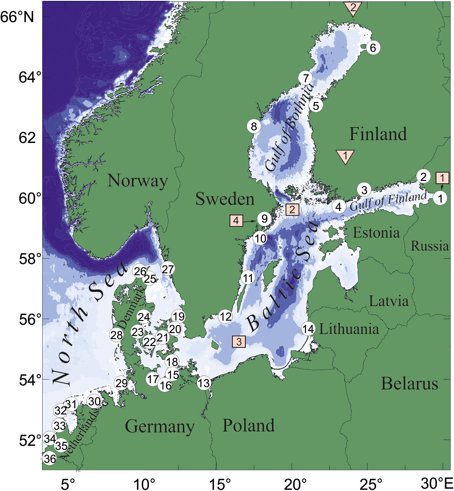
Figure 1. Locations of the tide gauge stations (white circles); the names of the stations are given in Table 1. The red squares indicate reanalysis grid point locations which were used to analyze (1) the air pressure from the NCEP/NCAR, (2) the air pressure from the ERA-Interim, (3) the air pressure and wind data from the 20th Century Reanalysis, and (4) the air pressure from the NCEP/CFSR. The red triangles show the location of the weather stations: (1) Pirkkala Tampere-Pirkkalan Lentoasema and (2) Pello Kk Museotie.

TABLE 1

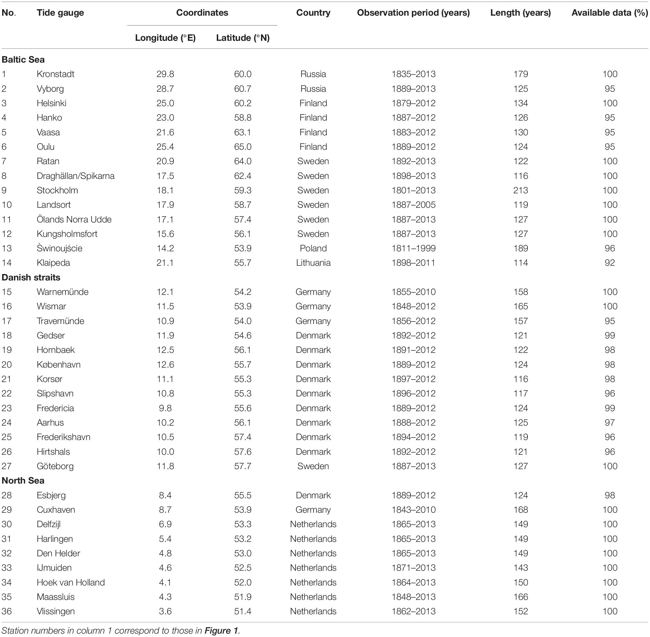
Table 1. The monthly MSL records in the Baltic Sea and the Southeast North Sea.

Hourly data sets of the air pressure at the sea level were obtained from the National Centers for Environmental Prediction Climate Forecast System Reanalysis (NCEP CFSR) from 1979 to 2010, with a spatial resolution at 0.5° × 0.5°. Monthly data sets of wind at 10 m and air pressure at the sea level were obtained from the 20th Century Reanalysis from 1871 to 2012. Monthly data sets of the air pressure at the sea level were obtained from the NCEP/NCAR Reanalysis (the National Centers for Environmental Prediction and the National Center for Atmospheric Research), from 1948 to 2015 and from the ERA-Interim reanalysis from 1979 to 2015. The Scandinavia pattern (SCAND) index was taken from the NOAA Climate Prediction Center from 1950 to 2015. The Scandinavian pattern consists of a primary circulation center over Scandinavia, with weaker centers of the opposite sign over Western Europe and eastern Russia/western Mongolia (Bueh and Nakamura, 2007). The Scandinavian (SCA) pattern was originally identified by Barnston and Livezey (1987) and previously referred to the Eurasia-1 pattern. The positive phase of this pattern is associated with positive height anomalies, sometimes reflecting major blocking anticyclones, over Scandinavia and western Russia, while the negative phase of the pattern is associated with negative height anomalies in these regions. The positive phase of the Scandinavian pattern is associated with below-average temperatures across central Russia and over western Europe. It is also associated with above-average precipitation across central and southern Europe and below-average precipitation across Scandinavia¹.

In this study, we used mean daily sea level pressure (SLP) from the weather stations of the European Climate Assessment (ECA) dataset (Klein Tank et al., 2002). Data and metadata are available at http://www.ecad.eu. Also, we used daily non-homogenous SLP observation data from the Stockholm Old Astronomical Observatory (59.35°N, 18.05°E) 1756−2012 (Moberg et al., 2002). These data were reduced to 0°C, normal gravity and MSL (Moberg et al., 2002).

To examine the periodical component in the sea level records we used the spectral analysis based on the fast Fourier transform (FFT). To obtain a better spectral resolution and the shortest confidence interval we stack the tide gauge data for three areas: the BS, the DS, and the NS. The procedure of stacking multistation data to enhance small signals has been used by seismologists to improve their estimates of the Earth’s free oscillation eigen frequencies (Gilbert and Dziewonski, 1975), and to search for short-period oceanic normal modes in the Pacific (Luther, 1982). Stacking is particularly useful in cases where the spatial dependence of the signal is known beforehand (Trupin and Wahr, 1990). For this procedure, we used rectangular spectral window. The window length N was 2048 months. The final sea level spectrum was calculated by averaging the periodograms counted for individual tide gauges without overlapping. The spectral resolution Δf was 0.0059 cycles per year (cpy). The Nyquist frequency was 6 cpy. The number of degrees of freedom was 28 for the BS, 26 for the DS, and 18 for the NS.

Spectral analyses of stochastic processes are commonly used in order to estimate the distribution of the sea level variance (energy) over the frequency. The spectrum can have a continuous character of the energy distribution (continuum) or the form of sharp delta-like peaks (discrete spectrum). It depends on the nature of the oscillations. For instance, tidal oscillations appear in the spectrum in the form of sharp peaks at the major tidal harmonic frequencies (K₁, O₁, M₂, S₂, etc., see Medvedev et al., 2013). The changes in sea level caused by the influence of alternating atmospheric pressure and wind fields at the sea surface are basically random in nature and have a noise spectrum as a continuous function of frequency.

To investigate temporal variations of low-frequency sea level oscillations the wavelet method was used. It was applied as in Torrence and Compo (1998), decomposing the time series into time-frequency space, in order to determine all dominant modes of the variability and the way these modes change in time. We used the continuous wavelet transform (Morlet wavelet). To analyze direct links between the sea level in different parts of these two seas and wind variations the wavelet coherence method was used (Grinsted et al., 2004; Jevrejeva et al., 2005).

Spectral Analysis

Figure 2 shows the spectra of sea level for three areas: the BS, the DS, and the NS. The major peak at all spectra corresponds to the annual cycle (Sa). The seasonal oscillations are the dominant feature of the long-period sea-level variability in most of the World Ocean. They are formed by the following components: air pressure and wind stress; seasonal variability of the water balance components, such as evaporation, precipitation, river runoff, water exchange with adjacent water bodies; steric effects (water temperature and salinity fluctuations); and long-period gravitational (astronomical) tides.

FIGURE 2

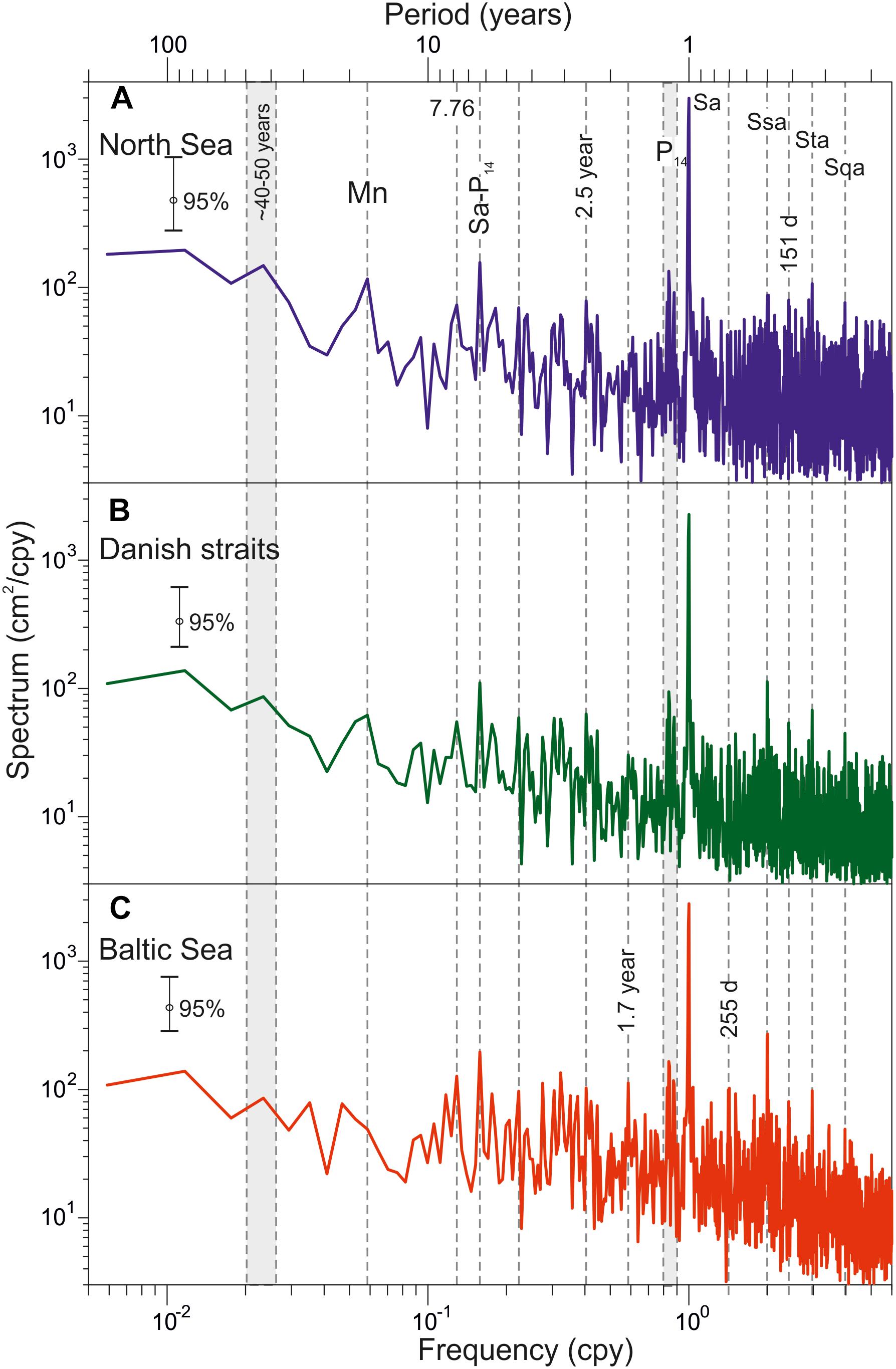
Figure 2. The low-frequency sea level spectra estimated from mean monthly sea level records in (A) the North Sea, (B) the Danish straits, and (C) the Baltic Sea. Labels “Mn,” “Sa,” “Ssa,” “Sta,” “Sqa,” and “P₁₄” mark nodal, annual, semiannual, terannual, quartoannual, and 14-month spectral peaks, respectively.

Higher seasonal components (semiannual – Ssa, terannual – Sta, quartoannual – Sqa) are caused by the asymmetry of the annual oscillations. In the NS, the amplitudes of higher seasonal harmonics are small and it is difficult to detect them in the background noise at the NS-spectrum (Figure 2A). To the contrary, in the BS these harmonics have significant amplitudes. The semiannual oscillations’ amplitudes for some years are about 25−30 cm (Medvedev, 2014). The maximum long-term amplitude (average climatic) of Ssa is 5 cm and is observed in the Åland Sea (Medvedev, 2014). The maximum of Sta harmonic is observed in the Åland Sea also (∼1.5 cm). The quartoannual harmonic is the highest in the Gulf of Finland, 2.7 cm (Medvedev, 2014). The spectral seasonal peaks Ssa, Sta and Sqa are well distinguished at BS-spectrum (Figure 2C). In the DS, the peaks Ssa, Sta, and Sqa are weaker than in the Baltic. According to the equilibrium theory of tides, the amplitude of the annual and semiannual gravitational constituents is ∼0.15 and 0.95 cm, in the BS (Lisitzin, 1974).

In the intra-annual frequency band, two stable spectral peaks with periods of 151 and 255 days can be identified in addition to the seasonal components (Sa, Ssa, Sta, Sqa). The first peak is localized in the DS and in the BS basin (Figures 2B,C). The second one is identified only on the sea level spectra within the BS (Figure 2C). The important feature of these spectral peaks is their sharp character, which corresponds to the deterministic processes.

The unknown origin wide peak with a period of 40−50 year and the nodal tide Mn peak with a period 18.61-year are distinguished in the low-frequency band. According to Wróblewski (2001), the amplitude of Mn in the BS is about 0.6–0.9 cm. It is close to the value of the static tide (Lisitzin, 1974). The nodal spectral peak is most pronounced at the NS-spectrum. In the BS, the nodal peak is not detected at the spectra.

It is possible to detect a frequency peak of about 0.84 cpy (14-month period) in all spectra of sea level oscillations (Figure 2). This harmonic corresponds to the Chandler frequency [Chandler wobble (CW)], which is the frequency of a free nutation of the Earth axis. It is considered, that the CWs cause weak tidal sea level oscillations in the World Ocean with a period of about 14 months. George Darwin called this oscillation the “pole tide” (Darwin, 1898).

The nutation of the Earth axis (the polar motion) affects not only the CW but also the annual component (with a frequency of 1 cpy). The annual polar component in the sea level oscillations hard to be detected, because seasonal oscillations of hydrometeorological origin are much stronger than this component. The influence of the sea level polar motion becomes apparent at lower frequencies. Thus, the sea level spectra for all three regions have a pronounced spectral peak with a 6.16-year period. Currie (1976), Trupin and Wahr (1990), and Hilmi et al. (2002) have also singled out this peak in the spectra. In their studies, the authors have not been able to determine the origin of this stable peak. It is likely that this peak is the result of interference of seasonal oscillations and the pole tide in the atmosphere, and has the frequency equal to the difference between the annual frequency and the Chandler frequency: f(Sa) – f(CW) = 1 cpy – 0.84 cpy = 0.16 cpy (6.16 year).

In the period band from 2 to 8 year, there is also a peak with a period of 7.76 year. In the interannual (intradecadal) frequency band, except for the already mentioned peaks, we can distinguish spectral peaks with periods of 2.5 and 1.7 year. The spectral peak with a period of 2.5 year is well pronounced at the NS spectra (Figure 2A) and the spectral peak with a period of 1.7 year is well pronounced at the BS spectra (Figure 2C). The oscillations in the 2.2–7.8-year band in individual sea level records have been associated with large-scale atmospheric circulation signals (Unal and Ghil, 1995; Jevrejeva et al., 2005). They generate sea level response through a number of processes: the direct influence of changes in atmospheric pressure, changes in wind stresses, and changes in atmosphere-ocean fluxes as well as storm surges (Jevrejeva et al., 2006). A peak with a period of 8.47 year can be identified in the spectrum of the BS level variability (Figure 2C). Its origin is explained by the lunar perigee.

Wavelet Analysis

To isolate different timescales of variability and analyze temporal changes of the sea level variance and periods, their behavior in time-frequency space have been examined using the Morlet wavelet analysis. Figure 3 shows the wavelet power spectrum for four sea level time series, displayed as a function of cycle period and time. The left axis is the Fourier period; the bottom axis shows time in years. We selected four tide gauges with long series of observations in different parts of the study region: IJmuiden (the NS), Gedser (the area of the DS), Stockholm (central part of the BS), and Kronstadt (the head of the Gulf of Finland). In general, the results of wavelet analysis confirm the results of spectral analysis of the prevalence of annual oscillations in the spectrum of low-frequency sea-level variability. The strong non-stationary behavior of the spectra is evident. The magnitude of the annual signal in the BS is much more variable from year to year compared with the NS. The period of the annual component demonstrates a significant change from year to year too. If the central period of this signal is strictly equal to 1 year for the NS, while the annual signal period in the BS experiences some changes from year to year. It must be caused by the influence of variations water exchange through DS and changes in the month of annual maximum river discharge (flood). Water exchange through straits causes large volume changes of the BS (Lehmann and Post, 2015) with the duration is about 40 days (Lehmann et al., 2012). These events cause the sea level rise by several dozens of centimeters (Soomere and Pindsoo, 2016) and may cause the variations of near-annual period. In some years (1910, 1990–2000), the magnitude of the annual signal does not exceed the background noise level. In 1990–2000 years the annual signal is absent in the wavelet spectra in the BS (Gedser, Stockholm, Kronstadt). The sea level variance in this decade cross to the 2–4-year band and semiannual oscillations. In wavelet power spectra of sea level variability, a semiannual component is higher in the BS but is difficult to detect in background noise in the NS. This is in good agreement with the results of the spectral analysis (Figure 2).

FIGURE 3

Figure 3. Wavelet power spectrum (Morlet) of the MSL for the (A) IJmuiden (NS), (B) Gedser (DS), (C) Stockholm, and (D) Kronstadt (BS). The contours are in variance units. The color bar represents normalized variances. In all panels, the black thin line is the cone of influence where edge effects might distort the picture, shown in a lighter shade.

The Chandler component of the sea level oscillations is not detected on these wavelet spectra due to the proximity of its period to the annual period. Perhaps variations of the annual component period shown in Figures 3B–D are caused by the influence of the pole tide, thereby increasing the period of the annual sea level component. To separate the annual and Chandler components, some other time-frequency analysis methods should be used, for example, multiple-filter technique (MFT) (Kulikov et al., 2004; Thomson and Emery, 2014). In Medvedev et al. (2017), the use of MFT with increasing frequency and decreasing time resolution allowed us to separate these two signals.

In all wavelet power spectra, especially in the BS, an increase in the variance of the oscillations with periods of about a 6–8 year has been detected since 1930. In the wavelet spectrum of the NS (Figure 3A), we can also distinguish an increase in sea level oscillations with a period of 16−20 year. It can be interpreted as a nodal tidal component (18.6 year) which was detected by the sea level spectrum in the NS (Figure 2A) and which was absent on the sea level spectra in the BS (Figure 2C). At Kronstadt, the wavelet power spectrum demonstrated an increase of the sea level variance in the 20−40-year band (Figure 3D).

Cross-Wavelet Analysis

To identify frequency bands within which time series of sea level in different sea parts are covarying, the wavelet coherence method was used (Grinsted et al., 2004; Jevrejeva et al., 2005, 2006). Synchronous time series of the monthly MSL for IJmuiden, Gedser, Stockholm, and Kronstadt were analyzed. Figure 4 shows wavelet coherence diagrams for four pairs of the sea level time series: (A) IJmuiden–Gedser, (B) IJmuiden–Stockholm, (C) Gedser–Stockholm, (D) Stockholm–Kronstadt. High coherence (>0.9) between IJmuiden–Gedser, and IJmuiden–Stockholm was revealed at the seasonal frequency and in the 2–8-year band in the second half of the 20th century. In general, the wavelet coherence for IJmuiden–Stockholm is higher than for IJmuiden–Gedser. It is caused by topographical features of the DS and the whole Baltic. The large basin in combination with topographic flow resistance in the connecting sounds act as a low-pass filter and lead to a reduction of amplitude (Andersson, 2002). The BS behavior is then that of a quarter-wave oscillation with a node at the entrance (Samuelsson and Stigebrandt, 1996), and the variance of the oscillations increases from the BS mouth toward the north because of the internal forcing (variations in local wind, air pressure, and density). Minimum amplitudes of the main long-period sea level components are observed in the DS: seasonal oscillations, pole tide as well as the total variance of the interannual sea level variability of the BS (Ekman, 1996; Medvedev, 2014, Medvedev et al., 2017). Weak coherence between the sea level oscillations in the North and BS s is detected for periods of more than 20 year.

FIGURE 4

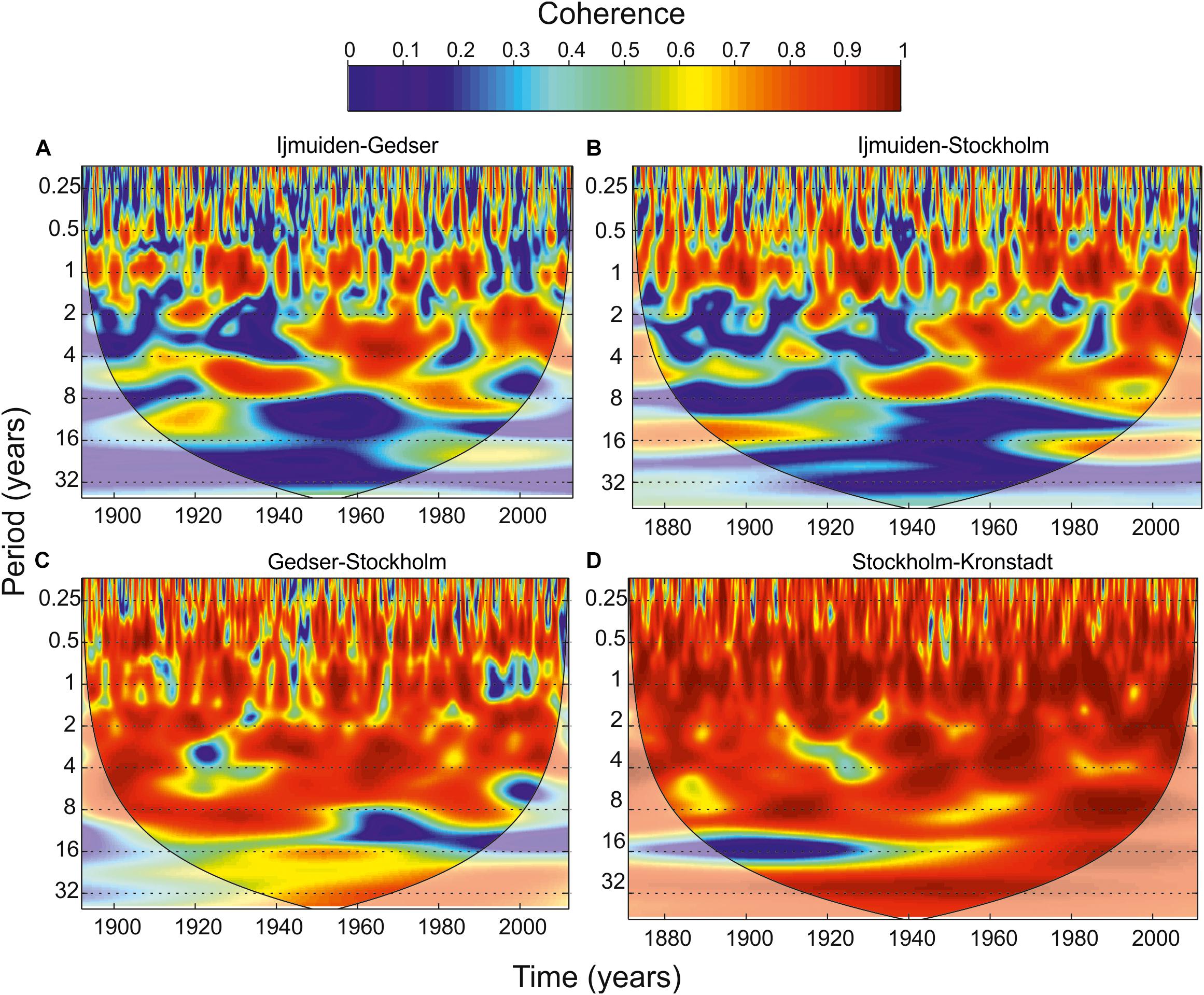
Figure 4. Wavelet coherence between (A) IJmuiden–Gedser, (B) IJmuiden–Stockholm, (C) Gedser–Stockholm, (D) Stockholm–Kronstadt. In all panels, the black thin line is the cone of influence where edge effects might distort the picture, shown in a lighter shade.

Very high coherence is observed between the sea level oscillations at different stations inside the BS over a wide range of periods. For Gedser–Stockholm, local coherence decreases in the 0.5–8-year band in single years and a general coherence decreases over periods of more than 10 year, but very high coherence (>0.8–0.9) was observed for Stockholm–Kronstadt in all of the studied frequency-time domain. Some local low coherence is found in the 0.16–0.5-year band. Permanently high coherence and close to zero phase difference are observed for periods of more than 0.5 year. It means that the sea level oscillations occur synchronously throughout the entire BS in a wide frequency range.

Because of the permanently high coherence in a wide frequency range, we should pay attention to the local coherence minima, which were found in the 3–4-year band during the 1910–1930 time period and for a 16-year signal during 1870–1930. The last wavelet peak in Figure 4 is of particular interest. The coherence in the 16-year oscillation of sea level between Stockholm and Kronstadt was weak from 1870 to the early 20th century, while from the 1940s the coherence for the 16-year oscillation increased substantially, exceeding 0.8 in the second half of the 20th century.

Mean sea level variations in the BS are closely related to the large-scale atmospheric circulation. Kauker and Meier (2003) showed that the variations of the NAO index describe up to 50% of the SLP variance over Northern Scandinavia, but only 10–30% of the variance over the BS. The SLP pattern shows a strong meridional gradient over the BS, causing strong zonal geostrophic winds, which influence sea level variations along the Baltic coast (Jevrejeva et al., 2005). In the present study, we examined the relationship between the sea level oscillations in the BS and wind variations. The wavelet spectrum of U-wind (zonal) component (Figure 5A) has the same structure as the wavelet spectra in Kronstadt and Stockholm: (1) an increase in the variance of the oscillations with periods of about a 6–8-year band has been detected since 1930; (2) the annual signal is absent in 1990–2000; and (3) the variance in 1990–2000 cross to the 2–4-year band and semiannual oscillations. The wavelet spectrum of the meridional (V) wind component (Figure 5B) has a significantly different structure than those of sea level (Figure 3).

FIGURE 5

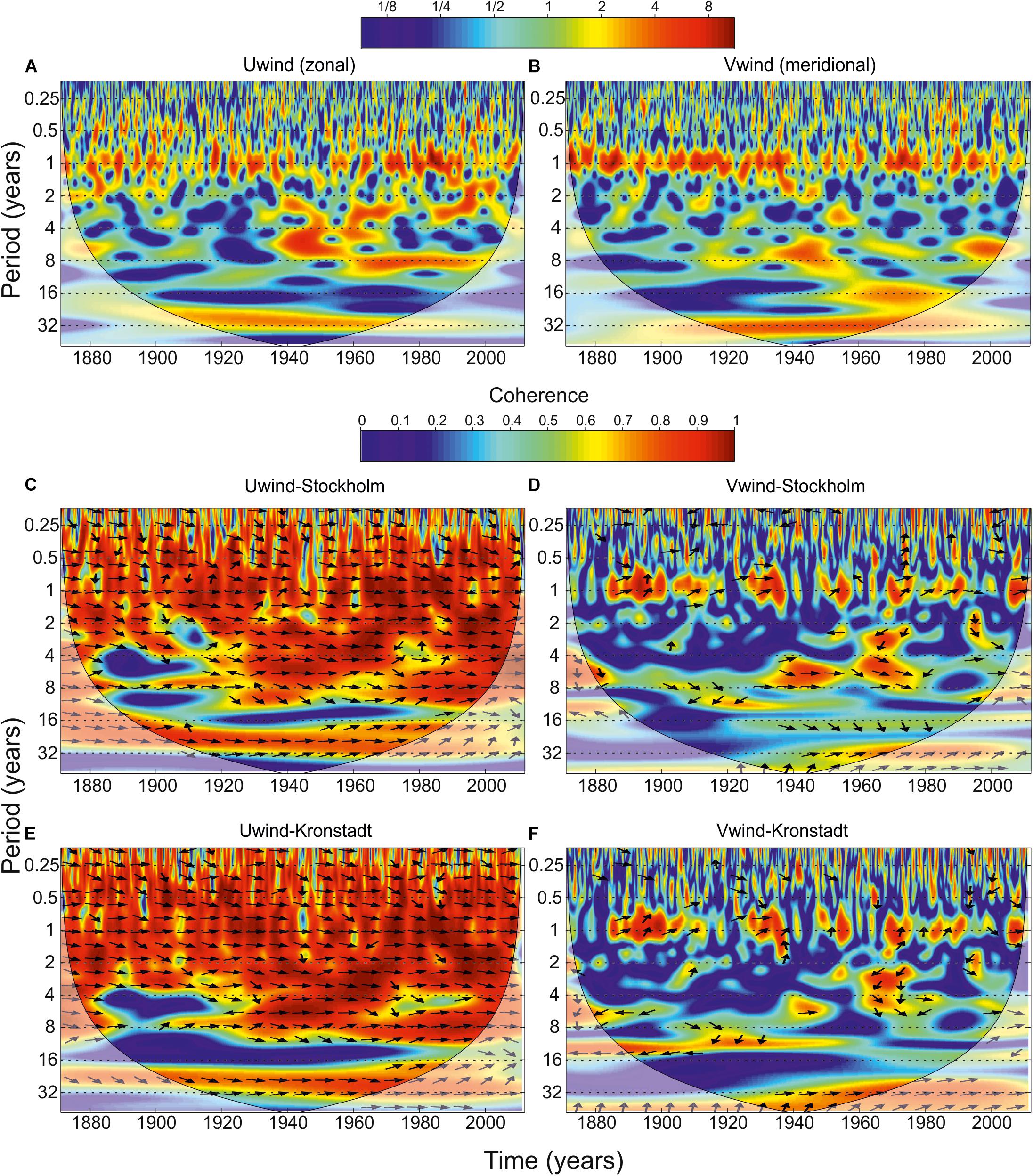
Figure 5. Wavelet power spectrum (Morlet) of mean monthly values of (A) zonal and (B) meridional components of wind speed from the 20th Century Reanalysis. Contours are in variance units. The color bar represents normalized variances. Wavelet coherence and the phase difference between (C) zonal wind – Stockholm, (D) meridional wind – Stockholm, (E) zonal wind – Kronstadt, and (F) meridional wind – Kronstadt. Contours are wavelet squared coherencies. The vectors indicate the phase difference. In all panels, the black thin line is the cone of influence where edge effects might distort the picture is shown as a lighter shade.

Figures 5C–F shows the wavelet coherence diagrams for time series of the monthly average zonal and meridional components of wind speed from the 20th Century Reanalysis (Compo et al., 2011) and the sea level oscillations in Stockholm and Kronstadt. The wavelet coherence diagrams in the 0.2–8-year band demonstrate a possible link between the zonal wind and the sea level variability at both tide gauge stations (coherence is 0.8–0.9). Both at Kronstadt and Stockholm the coherence decreases in the 4–8-year band in the late 19th – early 20th centuries and a permanently low coherence in the 14–20-year band. The cause of the first minimum is not clear, while the second coherence minimum appears to be caused by the astronomical origin of sea level oscillations with a well-defined nodal period of 18.6 year. The locally high coherence between meridional wind and sea level is observed for the annual component and in the 24–32-year period band.

Oscillation With a Period of 255 Days

In this study, we would like the particular attention to a vague spectral peak with a period of about 255 days. This spectral peak was also detected in the sea level spectra in different parts of the sea. Figure 6 shows the sea level spectra for four tide gauges: Kemi, Oulu, and Mäntyluoto in the Gulf of Bothnia, and Helsinki in the Gulf of Finland. These spectra were calculated without smoothing. Length of segments were 1116 months for Kemi, 1488 months for Oulu, 1228 months for Mäntyluoto, and 1608 months for Helsinki. The 95% significance levels were calculated according to the Chi-squared distribution of the variance of background noise. The peak with a period of 255 days at these spectra has their sharp character, which corresponds to the deterministic processes, and exceeds the 95% significance level.

FIGURE 6

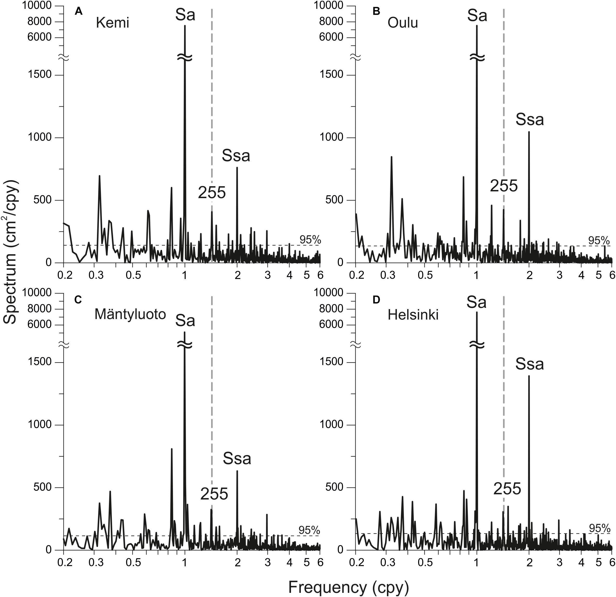
Figure 6. The sea level spectra estimated from mean monthly sea level records at (A) Kemi, (B) Oulu, (C) Mantyluoto, and (D) Helsinki. Labels “Sa,” “Ssa,” and “255” mark annual, semiannual, and 255-daily spectral peaks, respectively. Thin dashed lines show 95% significance level calculated according to Chi-squared distribution.

This peak was initially detected in spectral analysis of the results of numerical modeling of the sea level oscillations in the BS from 1979 to 2010 (Kulikov et al., 2015a). The numerical modeling of sea level variability in Kulikov et al. (2015a) was carried out using the closed basin approximation (closed DS), while the driving force in the model was due to the variations in atmospheric pressure and surface wind fields. The cause of the formation of this spectral component is therefore in the forcing. The atmospheric data for that model were taken from the NCEP/CFSR reanalysis (Saha et al., 2010).

We analyzed the spectral structure of the air pressure variations from different reanalyses. We used data at nodes near the Stockholm for ERA-Interim and NCEP/CFSR, near Kronstadt from NCEP/NCAR, and in the Bornholm Basin from 20th Century Reanalysis (see Figure 1). Spectra were calculated without smoothing. Length of segments were 418 months for ERA-Interim, 792 for NCEP/NCAR, 245448 h (∼336 months) for NCEP/CFSR, and 1376 months for 20th Century Reanalysis. The 95% significance levels were calculated according to the Chi-squared distribution of the variance of background noise. Figure 7D illustrates the spectra of fluctuations in atmospheric pressure at the NCEP/CFSR reanalysis node near Stockholm. On these spectra, the peak with a period of 255 days dominates significantly all other peaks, including the annual peak. The air pressure data from other reanalyses (NCEP/NCAR, 20th Century Reanalysis, ERA-Interim) were tested as well and a peak with a period of 255 days was also detected (Figures 7A–C). While in NCEP/NCAR, ERA-Interim reanalyses it is revealed better, than in 20th Century Reanalysis. However, it is presented at all the considered spectra and significantly exceeds the background noise level.

FIGURE 7

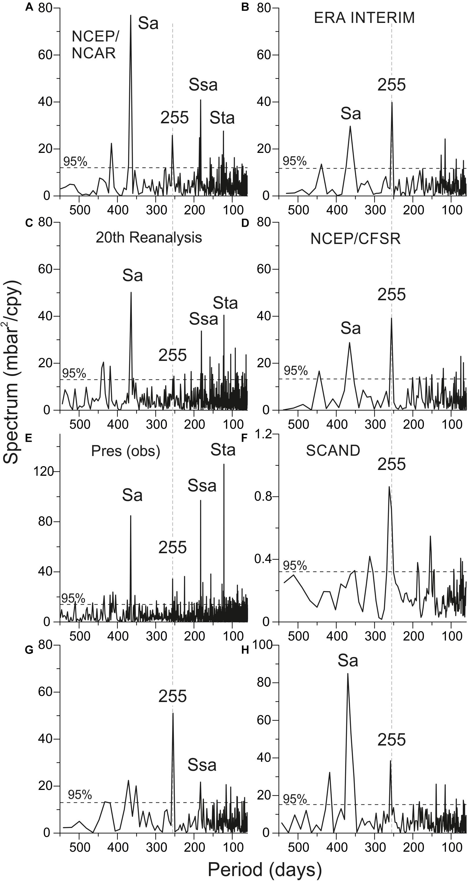
Figure 7. The air pressure spectra estimated from (A) NCEP/NCAR, (B) ERA-Interim, (C) 20th Century Reanalysis, (D) NCEP/CFSR reanalysis, air pressure observations at (E) Stockholm, (G) Pirkkala Tampere-Pirkkalan Lentoasema, (H) Pello Kk Museotie weather stations, and (F) Scandinavian index time series. Labels “Sa,” “Ssa,” “Sta,” and “255” mark annual, semiannual, terannual, and 255-daily spectral peaks, respectively. Thin dashed lines show 95% significance level calculated according to Chi-squared distribution.

As a next step, we have analyzed the air pressure observations from weather stations. We used daily observations of SLP from the Stockholm Old Astronomical Observatory during 1756–2012 (Moberg et al., 2002), and daily MSL pressure at weather stations from the ECA dataset (Klein Tank et al., 2002). Figure 7E shows air pressure spectrum for Stockholm. It was calculated by 93,868-month record without smoothing. The peak with a period of 255 days exceeds the background noise level. However, the main long-period components (annual, semiannual, and terannual) are larger. We have also checked air pressure spectra of observations at different weather stations in Europe. The peak with a period of 255 days was detected at weather stations of the Scandinavian region. Figures 7G,H show the air pressure spectra at Finnish weather stations Pirkkala Tampere-Pirkkalan Lentoasema (length of the record is 418 months) and Pello Kk Museotie (length of the record is 536 months), respectively. Spectra At the first station, the peak with a period of 255 days is significantly larger than all other peaks, including the annual peak. At Pello Kk Museotie, the peak with a period of 255 days is larger than other peaks, except for the annual peak, and significantly exceeds the background noise level.

At the conclusion of the study, we analyzed the Scandinavian pattern (SCAND index). We used the Kaiser-Bessel spectral window with a length of segment 370 months with half window overlaps and 6 degrees of freedom. The 95% significance levels were calculated according to the Chi-squared distribution of the variance of background noise. The peak with a period of 255 days is the main component of the spectrum of SCAND index (Figure 7F). One of its main features is its high quality (Q) factor, characteristic of deterministic geophysical processes, such as the tide. However, there are no frequencies in the expansion of the tidal potential that are close to 255 days. Consequently, the question of the nature of this peak remains open and requires further research.

Discussion

In the present study, we detected several peaks in the long-period sea level spectra in the NS and in the BS. In addition to the dominant annual and semiannual oscillations in the spectrum of long-period sea level variations, other peaks were also identified. In the period band less than 1 year, we detected the spectral peak with a period with 255 days. Our analyses revealed this peak in both the sea level spectra of the BS and in the spectra of the atmospheric processes. Vermeer et al. (1988) singled out the peak of the close period (242 days) at the sea level spectra of several tide gauges on the Finish coast of the BS. But Vermeer et al. (1988) did not give any explanation about the possible nature of this peak. O’Connor et al. (2000) reveled the peak with close period at the spectrum of the velocity of the zonal wind in the NS region, spatially averaged from NCEP/NCAR. But O’Connor et al. (2000) focused on the study of the pole tide and did not pay attention to the peak with a period of 255 days.

The pole tide peak with a period 14 months is one of the main distinguishing features of the sea level spectra of the BS and the NS. Typically, the pole tide has an equilibrium amplitude of about 0.5–0.7 cm. However, the pole tide amplitude estimated from the long tide gauge records in the North and Baltic Seas is 6–8 times higher than the equilibrium amplitude of the pole tide. The highest pole tide amplitude is in the Gulf of Finland is up to 6.5 cm (Medvedev et al., 2017). The pole tide does not have an exact fixed frequency, as the astronomical tide, and had significant temporal fluctuations in amplitudes and periods during the 19th and 20th centuries. If we use short sea level records for spectral analysis (30–40 year), we have a wide peak with a central frequency of 1/434 cpd in this band (Medvedev et al., 2014, 2017). If we apply spectral analysis to long records (>100 year), the spectral peak of the pole tide splits into a few separate components (Medvedev et al., 2014, 2017). The main pole tide peak has a period of ∼434 days (Figure 2). Also, we can distinguish pole tide peaks with periods of 417 and 443 days. The variations in the pole tide periods cause some spectral peaks in the pole tide frequency band. According to Munk and MacDonald (1960), the CW period varies in the interval by ±4%.

The spectral peak with a 6.16-year period is one of the strongest and most stable components of long-period sea level spectra for the BS and the NS in the period band from 1 year to a few decades. Currie (1976) and Trupin and Wahr (1990) have also singled out this peak in the spectra of the BS and the NS too. Vermeer et al. (1988) distinguished this peak at the sea level spectra of several tide gauges on the Finish coast of the BS. A similar signal with a period of 6–7 years was observed by Hilmi et al. (2002) in the sea level data in the Gulf of Saint Lawrence.

The nodal spectral peak Mn with a period 18.6-year is most pronounced at the sea level spectra in the NS (Figures 2A, 3A) and is not detected at the Baltic spectra (Figures 2C, 3C,D) and in the wavelet power spectra of the zonal wind (Figure 5A). The wavelet coherence between zonal wind and sea level in the BS is very low in these period band. It means that the nodal tide has the astronomical origin and has not the meteorological origin unlike the pole tide. Currie (1976) revealed a nodal peak in the sea level variations at tide gauges in the NS and DS region with amplitude up to 1.0–1.5 cm. At the Baltic stations, Currie (1976) did not find this peak. Only at Oulu, he found a similar peak, but the period of it was 20 year. Trupin and Wahr (1990) identified that the BS is the region where long-period noise seriously masks the 18.61-year signal. Currie (1976) also found the spectral peak with a solar-cycle period (10.5–11.5 year) in the low-frequency spectra in the NS and in the BS. However, in our results (Figure 2), this peak was not distinguished in each spectrum.

The sea level component with an 8.47-year period is probably linked to the lunar perigee. Munk and Cartwright (1966) showed evidence of the lunar perigee in influencing long-term water level variations. Hilmi et al. (2002) distinguished this peak at the sea level spectra of several tide gauges in the Gulf of Saint Lawrence.

Sea level oscillations with 12–30-year periods are probably linked to the propagation of the Atlantic water masses through the DS and decadal variability in the freshwater budget (Meier and Kauker, 2003; Jevrejeva et al., 2005). The oscillations in the 2.2–7.8-year band in sea level records have been associated with large-scale atmospheric circulation signals (Unal and Ghil, 1995; Jevrejeva et al., 2005). Changes in the atmospheric circulation would generate sea level response through a number of processes: the direct influence of changes in atmospheric pressure, changes in wind stresses, and changes in atmosphere-ocean fluxes as well as storm surges (Jevrejeva et al., 2005). The variations of these components could influence on the sea level variability.

As numerous studies (Andersson, 2002; Hünicke et al., 2015; Johansson and Kahma, 2016) shown the main factor of the Baltic long-period sea level formation is zonal wind. In this study, we describe the increase in the variance of sea level oscillations themselves and increased coherence between these oscillations and wind fluctuations in the BS since 1940s. Thus, high coherences have been detected between sea level variability in the North and Baltic Seas at the annual frequency and in the 2–8-year period band. The coherence between the 16-year sea level oscillations at Stockholm and Kronstadt was weak from 1870 to early 1900s, but increased substantially since the 1940s. Jevrejeva et al. (2005, 2006) have found a similar increase in various parts of the World Ocean. It was noted by Jevrejeva et al. (2006) that the amplitude of 3.5–13.9-year oscillations significantly increased since the 1940s in the Northeast and Northwest Atlantic, and in the East Pacific Jevrejeva et al. (2006) also showed that the noticeable increase of the influence (coherence) of the Arctic Oscillation on the sea level variability in the North Atlantic after 1940 is associated with the 2.2–13.9-year periodicity.

Conclusion

This research was primarily conceived to study the Baltic Sea level spectrum in the interval of periods from a few months to decades. Effective statistical methods of time series analysis have been applied to the long-term data from 36 tide gauges in the BS, the DS, and southeastern part of the NS, to examine the character of low-frequency sea level variability. The high spatial and temporal resolution of data allowed us to consider the features of the sea level spectrum in detail, to validate earlier conclusions and results of other investigators and to reveal some additional features which were previously unknown.

Our analysis supports the preliminary assumption that the sea level of the BS is governed mainly by changes in the zonal wind over this sea, which is one of the shallowest marginal seas. Extensive shallow-water areas provide favorable conditions for effective generation of intense wind-driven motions and creation of destructive storm surges in the Gulf of Finland and other shallow-water regions of the sea (e.g., Kulikov and Medvedev, 2013). The same effect appears to be responsible for the unusually high 14-month Chandler oscillations, wind-driven seasonal variations, and other long-period sea level variability (Medvedev et al., 2017). The presented analysis has enabled us to determine the nature of the low-frequency sea level variations as a response to the variable zonal winds in a very shallow sea.

In addition, our research has new findings. The cross-wavelet analysis shows that very high coherence (>0.8–0.9) over a wide range of periods from 2 months to 8–10 year is observed between the sea level oscillations inside the BS. It means that the sea level oscillations occur almost synchronously throughout the entire BS in a wide frequency range. However, there are some local coherence minima: in the 3–4-year band from 1910 to 1930 and for a 14–20-year band from 1870 to 1930. The wavelet spectrum of zonal wind component has the same structure as the wavelet spectra in Kronstadt and Stockholm: (1) an increase in the variance of the oscillations with periods of about a 6–8 year has been detected since 1930; (2) the annual signal is absent in 1990–2000 years; and (3) the variance in 1990–2000 years cross to the 2–4-year band and semiannual oscillations. The wavelet coherence diagrams demonstrate the strong relations of the zonal wind on the sea level variability at both tide gauge stations in the 0.2–8-year band. For example, the results for Kronstadt show a permanently low coherence in the 14–20-year band, which may be due to the astronomical origin of the sea level oscillations with the nodal period (18.6 year). Local high coherence between meridional wind and sea level variability are observed for the annual component and in the 24–32 year band.

The new and important result of this research is that we have identified in the BS separate periodic components, especially the peaks with the periods of 6.16 year and 255 days. Currie (1976), Trupin and Wahr (1990), and Hilmi et al. (2002) have also detected the 6.16-year sea level oscillation, but its origin was not explained. We propose that this peak is the result of interference between the seasonal oscillations and the pole tide in the atmosphere and has the frequency equal to the difference between the annual and the Chandler frequencies. This 255-day oscillation is the most intriguing result of this study. Our analyses revealed this peak in both the sea level spectra of the BS and in the spectra of the atmospheric processes. It is more pronounced in the air pressure variations from atmospheric reanalysis, especially in the ERA-Interim and NCEP/CFSR. This means that the reanalysis models reproduce this oscillation well enough. However, the origin of this 255-day oscillation is still unclear.

Author Contributions

IM coordinated the work on the manuscript, wrote the initial version of the manuscript, and prepared the figures. EK coordinated the work on the manuscript, and revised the text and figures substantially. IM and EK actively contributed to the development of the manuscript idea, writing, and preparation of figures.

Funding

This research was supported by the Russian Foundation for Basic Research, project 18-05-60250 (processing of reanalysis data) and the state assignment of IO RAS, theme 0149-2019-0005 (processing of tide gauge data).

Conflict of Interest

The authors declare that the research was conducted in the absence of any commercial or financial relationships that could be construed as a potential conflict of interest.

Footnotes

1. ^ https://www.cpc.ncep.noaa.gov/data/teledoc/scand.shtml

References

Andersson, H. C. (2002). Influence of long-term regional and large-scale atmospheric calculation on the Baltic sea level. Tellus A 54, 76–88. doi: 10.3402/tellusa.v54i1.12125

CrossRef Full Text | Google Scholar

Barnston, A. G., and Livezey, R. E. (1987). Classification, seasonality and persistence of low-frequency atmospheric circulation patterns. Mon. Weather Rev. 115, 1083–1126. doi: 10.1175/1520-0493(1987)115

CrossRef Full Text | Google Scholar

Bueh, C., and Nakamura, H. (2007). Scandinavian pattern and its climatic impact. Q. J. R. Meteorol. Soc. 133, 2117–2131. doi: 10.1196/annals.1446.014

PubMed Abstract | CrossRef Full Text | Google Scholar

Carlsson, M. (1997). Sea Level and Salinity Variations in the Baltic Sea – an Oceanographic Study Using Historical Data. Gothenburg: Göteborg University. Ph. D. thesis.

Google Scholar

Church, J. A., and White, N. J. (2011). Sea level rise from the late 19th to the early 21st century. Surv. Geophys. 32, 585–602. doi: 10.1007/978-94-007-2063-3_17

CrossRef Full Text | Google Scholar

Compo, G. P., Whitaker, J. S., Sardeshmukh, P. D., Matsui, N., Allan, R. J., Yin, X., et al. (2011). The twentieth century reanalysis project. Q. J. R. Meteorol. Soc. 137, 1–28.

Google Scholar

Currie, R. G. (1976). The spectrum of sea level from 4 to 40 years. Geophys. J. R. Astron. Soc. 46, 513–520. doi: 10.1111/j.1365-246x.1976.tb01245.x

PubMed Abstract | CrossRef Full Text | Google Scholar

Darwin, G. H. (1898). The Tides and Kindred Phenomena in the solar System. New York, NY: Houghton Mifflin and company.

Google Scholar

Ekman, M. (1996). A common pattern for interannual and periodical sea level variations in the Baltic Sea and adjacent waters. Geophysica 32, 261–272.

Google Scholar

Ekman, M. (2007). A Secular Change in Storm Activity Over the Baltic Sea Detected Through Analysis of Sea Level Data. Small Publ Hist Geophys. Åland Islands: Summer Institute for Historical Geophysics.

Google Scholar

Ekman, M. (2009). The Changing Level of the Baltic Sea During 300 Years: a Clue to Understanding the Earth. Åland Islands: Summer Institute for Historical Geophysics.

Google Scholar

Ekman, M., and Stigebrandt, A. (1990). Secular change of the seasonal variation in sea level and of the pole tide in the Baltic Sea. J. Geophys. Res. 95, 5379–5383.

Google Scholar

Gilbert, F., and Dziewonski, A. M. (1975). An application of normal mode theory to the retrieval of structural parameters and source mechanisms from seismic spectra. Philos. Trans. R. Soc. Lon. A 278, 187–269. doi: 10.1098/rsta.1975.0025

CrossRef Full Text | Google Scholar

Grinsted, A., Moore, J. C., and Jevrejeva, S. (2004). Application of the cross wavelet transform and wavelet coherence to geophysical time series. Nonlinear Process. Geophys. 11, 561–566. doi: 10.5194/npg-11-561-2004

CrossRef Full Text | Google Scholar

Hammarklint, T. (2009). Swedish Sea Level Series – A Climate Indicator. Norrköping: Swedish Meteorological and Hydrological Institute.

Google Scholar

Hilmi, K., Murty, T., El Sabh, M. I., and Chanut, J.-P. (2002). Long-Term and short-term variations of sea level in Eastern Canada: a review. Mar. Geodesy 25, 61–78. doi: 10.1080/014904102753516732

CrossRef Full Text | Google Scholar

Holgate, S. J., Matthews, A., Woodworth, P. L., Rickards, L. J., Tamisiea, M. E., Bradshaw, E., et al. (2013). New data systems and products at the permanent service for mean Sea level. J. Coast. Res. 29, 493–504.

Google Scholar

Hünicke, B., Zorita, E., Soomere, T., Madsen, K. S., Johansson, M., and Suursaar, Ü (2015). Recent Change–Sea Level and Wind Waves. In Second Assessment of Climate Change for the Baltic Sea Basin. Cham: Springer, 155–185.

Google Scholar

Jevrejeva, S., Grinsted, A., Moore, J. C., and Holgate, S. (2006). Nonlinear trends and multiyear cycles in sea level records. J. Geophys. Res. 111:C09012.

Google Scholar

Jevrejeva, S., Moore, J. C., Woodworth, P. L., and Grinsted, A. (2005). Influence of large scale atmospheric circulation on the European sea level: results based on the wavelet transform method. Tellus A 57, 129–149.

Google Scholar

Johansson, M., and Kahma, K. K. (2016). On the statistical relationship between the geostrophic wind and sea level variations in the Baltic Sea. Coast. Res. 21, 25–43.

Google Scholar

Kauker, F., and Meier, H. E. M. (2003). Modeling decadal variability of the Baltic Sea: 1. Reconstructing atmospheric surface data for the period 1902–1998. J. Geophys. Res. 108:3267. doi: 10.1029/2003JC001797

CrossRef Full Text | Google Scholar

Klein Tank, A. M. G., Wijngaard, J. B., Können, G. P., Böhm, R., Demarée, G., Gocheva, A., et al. (2002). Daily dataset of 20th-century surface air temperature and precipitation series for the European Climate Assessment. Int. J. of Climatol. 22, 1441–1453. doi: 10.1002/joc.773

CrossRef Full Text | Google Scholar

Kulikov, E. A., and Medvedev, I. P. (2013). Variability of the baltic sea level and floods in the gulf of finland. Oceanology 53, 145–151. doi: 10.1134/s0001437013020094

CrossRef Full Text | Google Scholar

Kulikov, E. A., Fain, I. V., and Medvedev, I. P. (2015a). Numerical modeling of anemobaric fluctuations of the Baltic Sea level. Russ. Meteorol. Hydrol. 40, 100–108. doi: 10.3103/s1068373915020053

CrossRef Full Text | Google Scholar

Kulikov, E. A., Medvedev, I. P., and Koltermann, K. P. (2015b). Baltic sea level low-frequency variability. Tellus A 67:25642. doi: 10.3402/tellusa.v67.25642

CrossRef Full Text | Google Scholar

Kulikov, E. A., Rabinovich, A. B., and Carmack, E. C. (2004). Barotropic and baroclinic tidal currents on the Mackenzie shelf break in the southeastern Beaufort Sea. J. Geophys. Res. 109:C05020. doi: 10.1029/2003JC001986

CrossRef Full Text | Google Scholar

Lehmann, A., Myrberg, K., and Höflich, K. (2012). A statistical approach to coastal upwelling in the Baltic Sea based on the analysis of satellite data for 1990–2009. Oceanologia 54, 369–393. doi: 10.5697/oc.54-3.369

CrossRef Full Text | Google Scholar

Lehmann, A., and Post, P. (2015). Variability of atmospheric circulation patterns associated with large volume changes of the Baltic Sea. Adv.Sci.Res. 12, 219–225. doi: 10.5194/asr-12-219-2015

CrossRef Full Text | Google Scholar

Lisitzin, E. (1974). Sea Level Changes. Amsterdam: Elsevier.

Google Scholar

Luther, D. S. (1982). Evidence of a 4–6 day barotropic, planetary oscillation of the Pacific Ocean. J. Phys. Oceanogr. 12, 644–657. doi: 10.1175/1520-0485(1982)012<0644:eoadbp>2.0.co;2

CrossRef Full Text | Google Scholar

Medvedev, I. P. (2014). Seasonal fluctuations of the Baltic sea level. Russ. Meteorol. Hydrol. 39, 814–822. doi: 10.3103/s106837391412005x

CrossRef Full Text | Google Scholar

Medvedev, I. P., Rabinovich, A. B., and Kulikov, E. A. (2013). Tidal oscillations in the Baltic Sea. Oceanology 53, 526–538. doi: 10.1134/s0001437013050123

CrossRef Full Text | Google Scholar

Medvedev, I. P., Rabinovich, A. B., and Kulikov, E. A. (2014). Pole tide in the Baltic Sea. Oceanology 54, 121–131. doi: 10.1134/s0001437014020179

CrossRef Full Text | Google Scholar

Medvedev, I. P., Rabinovich, A. B., and Kulikov, E. A. (2017). The pole tide/14-month oscillations in the Baltic Sea during the 19th and 20th centuries: spatial and temporal variations. Cont. Shelf Res. 137, 117–130. doi: 10.1016/j.csr.2017.02.001

CrossRef Full Text | Google Scholar

Meier, H. E. M., and Kauker, F. (2003). Modeling decadal variability of the Baltic Sea: 2. Role of freshwater inflow and large-scale atmospheric circulation for salinity. J. Geophys. Res. 108:3368. doi: 10.1029/2003JC001799

CrossRef Full Text | Google Scholar

Moberg, A., Bergström, H., Ruiz Krigsman, J., and Svanered, O. (2002). Daily air temperature and pressure series for Stockholm (1756-1998). Clim. Change 53, 171–212. doi: 10.1007/978-94-010-0371-1_7

CrossRef Full Text | Google Scholar

Munk, W. H., and Cartwright, D. E. (1966). Tidal spectroscopy and prediction. Phil. Trans. Roy. Soc. London. Ser. A 259, 533–581.

Google Scholar

Munk, W. H., and MacDonald, G. J. F. (1960). The Rotation of the Earth. New York: Cambridge University Press.

Google Scholar

O’Connor, W. P., Chao, B. F., Zheng, D., and Au, A. Y. (2000). Wind stress forcing of the North Sea ‘Pole Tide’. Geophys. J. Int. 142, 620–630. doi: 10.1046/j.1365-246x.2000.00184.x

CrossRef Full Text | Google Scholar

Peltier, W. R. (2004). Global glacial isostasy and the surface of the ice-age Earth: the ICE-5G (VM2) model and GRACE. Annu. Rev. Earth Planet. Sci. 32, 111–149. doi: 10.1146/annurev.earth.32.082503.144359

CrossRef Full Text | Google Scholar

Richter, A., Groh, A., and Dietrich, R. (2011). Geodetic observation of sea level change and crustal deformation in the Baltic Sea region. Phys. Chem. Earth 5, 43–53. doi: 10.1016/j.pce.2011.04.011

CrossRef Full Text | Google Scholar

Saha, S., Moorthi, S., Pan, H.-L., Wu, X., Wang, J., Nadiga, S., et al. (2010). The NCEP climate forecast system reanalysis. Bull. Am. Meteorol. Soc. 91, 1015–1057.

Google Scholar

Samuelsson, M., and Stigebrandt, A. (1996). Main characteristics of the long-term sea level variability in the Baltic Sea. Tellus A 48, 672–683. doi: 10.1034/j.1600-0870.1996.t01-4-00006.x

CrossRef Full Text | Google Scholar

Soomere, T., and Pindsoo, K. (2016). Spatial variability in the trends in extreme storm surges and weekly-scale high water levels in the eastern Baltic Sea. Cont. Shelf Res. 115, 53–64. doi: 10.1016/j.csr.2015.12.016

CrossRef Full Text | Google Scholar

Thomson, R. E., and Emery, W. J. (2014). Data Analysis Methods in Physical Oceanography, Third and revised edition. New York, NY: Elsevier.

Google Scholar

Torrence, C., and Compo, G. P. (1998). A practical guide to wavelet analysis. Bull. Am. Meteorol. Soc. 79, 61–78.

Google Scholar

Trupin, A., and Wahr, J. (1990). Spectroscopic analysis of global tide gauge sea level data. Geophys. J. Int. 100, 441–453. doi: 10.1111/j.1365-246x.1990.tb00697.x

CrossRef Full Text | Google Scholar

Unal, Y. S., and Ghil, M. (1995). Interannual an interdecadal oscillation patterns in sea level. Clim. Dyn. 11, 255–278. doi: 10.1007/bf00211679

CrossRef Full Text | Google Scholar

Vermeer, M., Kakkuri, J., Mälkki, P., Boman, H., Kahma, K. K., and Leppäranta, M. (1988). Land uplift and sea level variability spectrum using fully measured monthly means of tide gauge readings. Finn. Mar. Res. 256, 1–75.

Google Scholar

Wahl, T., Haigh, I. D., Woodworth, P. L., Albrecht, F., Dillingh, D., Jensen, J., et al. (2013). Observed mean sea level changes around the North Sea coastline from 1800 to present. Earth Sci. Rev. 124, 51–67. doi: 10.1016/j.earscirev.2013.05.003

CrossRef Full Text | Google Scholar

Wróblewski, A. (2001). Lunar nodal tide in the Baltic Sea. Oceanologia 43, 99–112.

Google Scholar