High Resolution Mapping of Ice Mass Loss in the Gulf of Alaska From Constrained Forward Modeling of GRACE Data

Introduction

Glaciers represent 68.9% of fresh water resources worldwide. In many regions of the world, people rely on glacier meltwater for agriculture, hydropower, industries, and municipal water requirements (Chen and Ohmura, 1990; Blanchon and Boissière, 2009). However, over the last decades, the glacier mass losses have raised concerns in and beyond the research communities. Climate change leads to important reductions in glacial water storage. Glaciers have an important influence on sea level rise; hence, their melt threatens the living environment of costal dwellings. Jin and Feng (2016) estimated the contribution of glacial melt to sea level change between 2003 and 2012 at 1.94 ± 0.29 mm/year. From 120,000 glaciers available in the World Glacier Inventory, Radić and Hock (2011) estimated that the total volume loss could be as much as 21 ± 6% by 2100, leading to a total sea level rise of 124 ± 37 mm.

Numerous studies focused on estimating the ice mass loss over specific continents, regions, or Mountain ranges. For example, Larsen et al. (2007) investigated glacier changes in southeast Alaska and northwest British Columbia over the period 1948–2000 and 1982/1987–2000, respectively. By combining the results from these periods, they estimated an average ice mass loss rate of 16.7 ± 4.4 Gt/year. In the Canadian Rocky Mountains, Castellazzi et al. (2019) estimated a total of 43 Gt of glacial mass loss over the period 2002–2015. Over the entire Gulf Of Alaska (GOA) area, Gardner et al. (2013) found 50 ± 17 Gt/year of glacier mass loss based on several published GRACE estimates over the period 2003–2009. Berthier et al. (2010) obtained 41.63 ± 8.6 Gt/year of glacier ice loss from Digital Elevation Models (DEM) for the period 1962–2006. Larsen et al. (2015) used airborne altimetry to estimate glacier mass loss rate over the period 1994–2013 and found 75 ± 11 Gt/year.

Gravity data provides direct information over ice mass changes, as the link between gravity and mass is direct and requires no calibration. In situ gravity measurements are labor-intensive, costly to acquire, and point-based; while satellite gravity data are limited in resolution due to the sensing distance. Since 2002, the United States (NASA) and the German (DLR) space agencies have led the Gravity Recovery And Climate Experiment (GRACE) mission. It aims at monitoring the variations of the Earth’s gravity field with a temporal resolution of a few days to a month, with a spatial resolution of ± 400 km (Tapley et al., 2004; Ramillien et al., 2017). The variations in the Earth’s mass distribution cause changes in the gravity field (Wahr et al., 1998). Thus, by mapping the variations of the gravitational field, GRACE monitors the Earth’s mass distribution. The mass redistribution obtained from GRACE data contains changes in Terrestrial Water Storage (TWS), and oceanic mass (Wahr et al., 1998; Chen et al., 2006). Yirdaw et al. (2009) noted that the GRACE mission estimates could be used to monitor the rate of change of TWS over large spatial scales. Ramillien et al. (2017) further indicated that continental hydrology is one of the main applications of GRACE data. The variation of TWS aggregates changes in surface water, soil moisture, ground water, snow, and ice. Jin and Zou (2015) used GRACE data to estimate a high-precision glacier mass dynamics in Greenland. In the GOA region, GRACE data have already been used to estimate glacier mass loss (Tamisiea et al., 2005; Chen et al., 2006; Arendt et al., 2008, 2009, 2013; Luthcke et al., 2008; Baur et al., 2013; Beamer et al., 2016; Wahr et al., 2016; Jin et al., 2017).

Two main types of GRACE Level-3 solutions are used in hydrological applications. There are unconstrained solutions, relying on de-stripping and Spherical Harmonics (SH) truncation, and constrained solutions often relying on regularization or stabilization. Among the later, mascon solutions, obtained after inverting the GRACE signal into a mass change for each spatial unit (“mascon”) of a predefined grid, have become particularly popular over the last years (e.g., Save et al., 2016). Meanwhile, the unconstrained GRACE Spherical Harmonics (SH) solutions present errors at high spatial frequencies (e.g., N > 60 or 300 km) and North-South stripes mainly due to gravitational model corrections, instrument errors, and gaps in data coverage. Destriping, truncation, and filtering are usually applied on these Level-2 solutions to reduce high frequency errors and to eliminate stripes. The challenge of using GRACE data to investigate hydrological fluxes, such as mass variations at the glacier scale, lies in the low spatial resolution (300/400 km) and the inability to discriminate close masses. Leakage effects are inherent to the GRACE sensing strategy, and are accentuated by the truncation and filtering used to “clean” the monthly gridded mass changes. This makes GRACE data prone to large errors when considering areas below 200,000 km² (e.g., Longuevergne et al., 2010). To overcome this problem, several authors combined GRACE data with other sources of information (e.g., Castellazzi et al., 2018, 2019).

Different strategies such as scaling approach, additive approach, multiplicative approach, and unconstrained or constrained forward modeling approaches permit to partially restore the signal loss (Long et al., 2016). A constrained inversion method can also be applied to improve the spatial resolution of GRACE data (Farinotti et al., 2015; Long et al., 2016; Castellazzi et al., 2018). Chen et al. (2015) used forward modeling to restore the GRACE signal amplitude of Antarctic ice and glacier loss due to the noise reduction. Long et al. (2016) showed that a constrained forward modeling can recover the distribution details of the GRACE signal. Farinotti et al. (2015) estimated the glacier mass loss in the Tien Shan (China) by subtracting the non-glacier contributions from the total mass change. They used an inversion method with a priori information about the glacier spatial distribution in area subdivisions (i.e., mascon and sub-mascon). By improving GRACE spatial resolution, their results are comparable to those derived from altimetry data and glacial melt modeling (e.g., the Cold Regions Hydrological Model—Pomeroy et al., 2007—and the Distributed Enhanced Temperature Index Model—Hock, 1999). Studying groundwater depletion in Central Mexico, Castellazzi et al. (2016, 2018) improved the GRACE spatial resolution using InSAR-derived ground-displacement maps to constrain the Forward Model (FM). They subtracted groundwater contributions from other components of TWS, built a distribution map of groundwater depletion using InSAR, and focused GRACE data over it. The potential of separating masses depends on the size, separation, and amplitude of the masses, as well as on the available constraining data and their efficiency in explaining the low resolution GRACE signal.

Although several authors have injected ancillary data into GRACE post-processing to improve the resolution, there is still a need to assess how constrained modeling improves the interpretation of GRACE data versus simplistic approaches such as spatial averaging (e.g., usually over watersheds or regions). While few studies already tested how constrained FM can help interpreting GRACE data, case studies are still lacking and more importantly, the limits of the procedure are still relatively unknown. In this study, we apply this procedure to build a high resolution ice mass loss map from GRACE data over a large range of melting glaciers in the GOA. In that perspective, we use several GRACE solutions, apply a spatial constraint to focus the signal, and provide a high spatial resolution map of ice mass loss over the study area.

Study Area

Our study area is delimited by zone 11 (Figure 1). The area was selected to cover the glaciers of the GOA and to include a stretch of ∼300 km of the surroundings to account for spatial leakages inherent to the GRACE signal. During the last decade, different studies used GRACE data to estimate glacier mass across the same region (Figure 1).

FIGURE 1

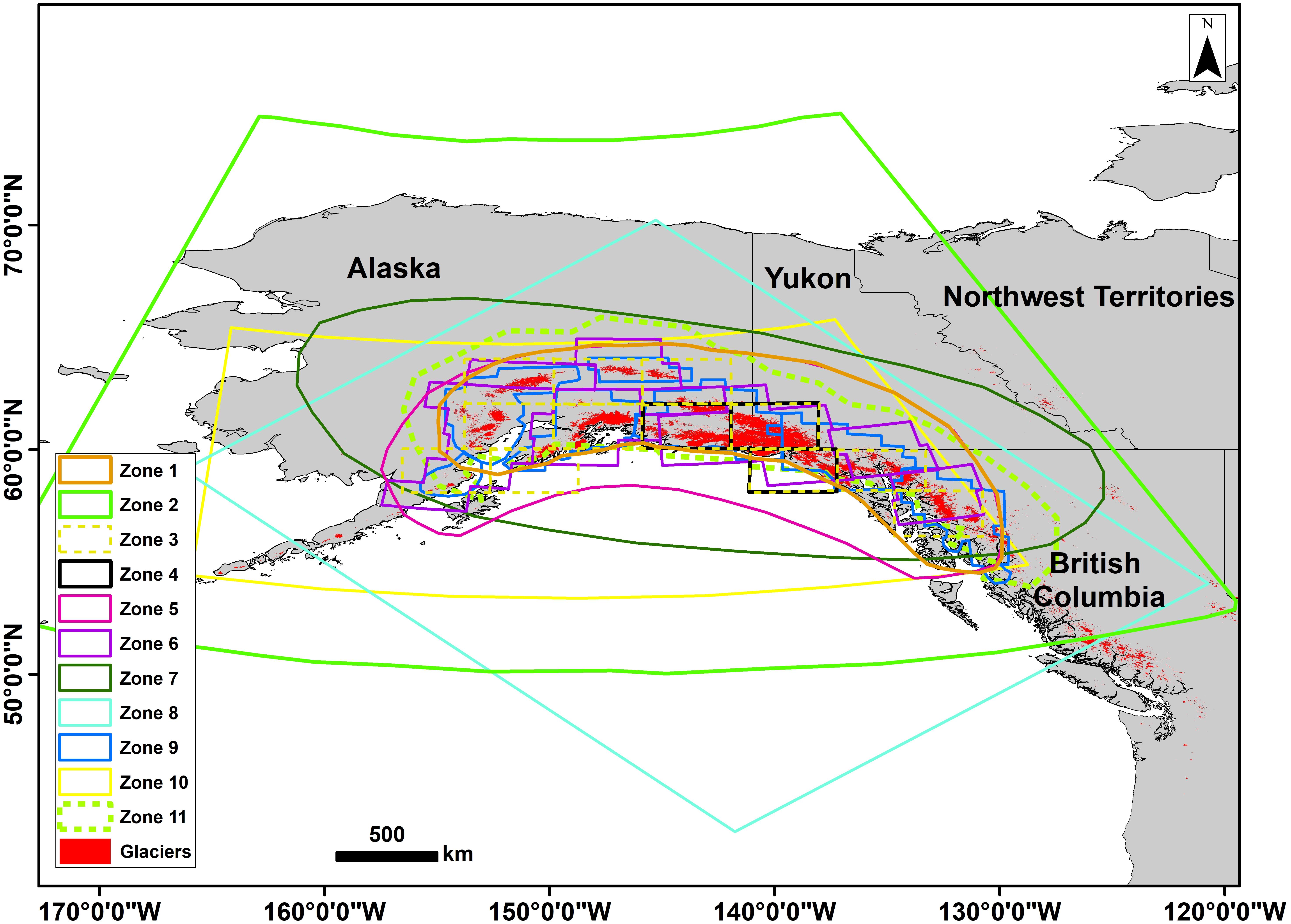
Figure 1. Glaciers of the GOA and footprints of the study area considered in studies using GRACE data to assess glacier melt. The study area considered here is identified as Zone 11.

There are discrepancies in mass losses estimated over the GOA. Most authors obtain values ranging from −47 to −110 Gt/year of glacial mass change (Figure 1 and Table 1). These studies consider different spatial extents and data time-periods. For example, the total surface coverage considered by Tamisiea et al. (2005) is 701,000 km², while Beamer et al. (2016) consider 420.300 km². The first three studies show higher values of mass loss (Tamisiea et al., 2005; Chen et al., 2006; Luthcke et al., 2008) than those more recent (Baur et al., 2013; Beamer et al., 2016; Wahr et al., 2016; Jin et al., 2017). It is potentially due to the relatively short GRACE time-series available at that time and the higher uncertainties in the earlier releases of GRACE data. In addition, variations in the GRACE data processing strategy, including levels of filtering and Spherical Harmonic (SH) truncation, might also contribute to discrepancies between studies. For example, some studies used unconstrained solutions (Tamisiea et al., 2005; Chen et al., 2006; Baur et al., 2013; Jin et al., 2017). Other authors used mascon solutions at different spatial and temporal resolutions (Arendt et al., 2008, 2009, 2013; Luthcke et al., 2008, 2013; Jacob et al., 2012; Beamer et al., 2016; Wahr et al., 2016). Tamisiea et al. (2005) used unconstrained solutions completed up to SH degree and order 70. Other authors used SH degree and order up to 60 (Chen et al., 2006; Baur et al., 2013; Jin et al., 2017). Jin et al. (2017) applied a Gaussian filter with a radius of 300 km while the aforementioned studies used a radius of 500 km. Using a scaling factor approach, Tamisiea et al. (2005) reduced the GRACE signal attenuation and leakage. A forward modeling approach was also used by several authors to restore signal leakages from coastal glaciers to the ocean (Baur et al., 2013; Jin et al., 2017).

TABLE 1

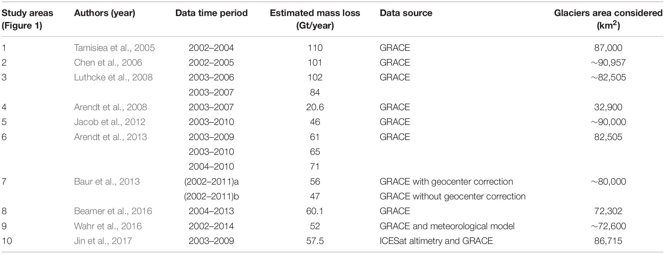
Table 1. Estimates of glacier mass loss in the GOA according to different authors.

Some authors also used auxiliary data to complement GRACE observations. Remote sensing of ice surface elevation (e.g., ICESat NASA, airborne laser altimetry) was combined with GRACE data (Arendt et al., 2008, 2013; Jin et al., 2017). Meteorological models also contributed to GRACE science (Arendt et al., 2009; Wahr et al., 2016). Some authors combined remote sensing and meteorological data to enrich and validate glacier mass loss estimates (Arendt et al., 2013; Luthcke et al., 2013). Beamer et al. (2016) developed hydrological models and compared their results with the airborne altimetry and GRACE data.

Data and Methods

Glacier Data and Mascon Delineation

Glaciers are delimited using the GLIMS Glacier Database released on 27/10/2017 and available online¹ (GLIMS and NSIDC, 2005, updated in 2013). It is a continuation of the World Glacier Inventory (Raup et al., 2007) which compiles different sources: satellite imagery data, historical information from maps, and aerial photography. Recently, the GLIMS glacier Database was merged with the Randolph Glacier Inventory (RGI). According to Pfeffer et al. (2014), this combination was performed to support the fifth report of the Intergovernmental Panel on Climate Change. While the GLIMS database may contain errors, it is, at least for our study area, in good agreement with the glacier inventory of Alaska and northwest Canada proposed by Kienholz et al. (2015). According to GLIMS, the total glacier cover in the GOA area was around 90,000 km² in 2013 (Figure 2).

FIGURE 2

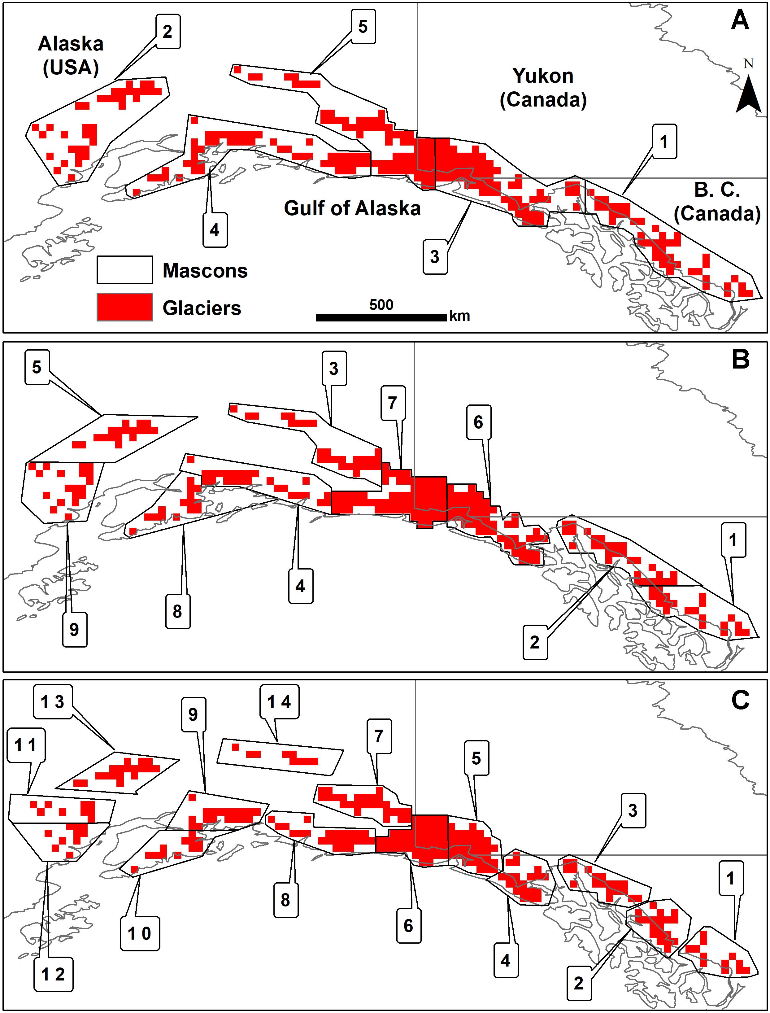
Figure 2. Glacier distribution map used to focus GRACE trend maps. Three arbitrary mascon delineations are presented: (A) 5 mascons with an average area of ∼55,000 km², (B) 9 mascons with an average area of ∼30,000 km², and (C) 14 mascons with an average area of ∼20,000 km².

To ease data handling and make this dataset compatible with other GRACE grids used in this study, the glacier distribution was resampled to a 0.25° grid (∼28 km by ∼14 km pixels; Figure 2). The resampling is performed using the following steps: (1) creation of a global 0.25° raster; (2) overlay of the glacier footprint (taken as polygons) from the GLIMS data on the raster; and (3) creation of the distribution map. In the latter step, we consider that a pixel from step (1) contains glacial masses if its center is within a glacier polygon from GLIMS.

Separating the contribution from a set of small masses to a low resolution signal (such as GRACE) can be challenging and the success relies principally on the initial resolution, the final resolution, the size of the masses, the distance separating them, and the amplitude of the changes for each mass. Their spatial separation is important, close masses being harder to discriminate than those spatially distant. To test the separation of the signal into a set of contributing masses, we considered three different spatial distributions of mass at different resolutions (Table 2). Each area delimiting a mass is referred to as a mascon (mass concentration area).

TABLE 2

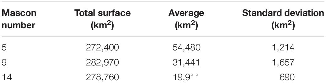
Table 2. Description of the three mascon delineations.

The GOA glacial mass losses are spatially heterogeneous due to the difference in size of glaciers, local hypsometry, and climate (i.e., temperature and precipitation; Frans et al., 2018; Huss and Hock, 2018). For simplification, we assumed a uniform distribution of ice mass loss within each mascon and test this assumption through a synthetic test (section “Simulation With Synthetic Data”). This assumption has been used in other areas prone to ice mass loss by Chen et al. (2009) and in Farinotti et al. (2015).

GRACE TWS Data

Three versions of Level-3 GRACE data in Water Thickness Equivalent (WTE) are considered. The first solution is the stabilized solution from the Space Geodesy Research Group (GRGS RL04²) available up to SH degree and order 90. The second is an unconstrained solution from the Center for Space Research (CSR RL06) complete up to SH degree and order 96 and de-striped/filtered in a single step by applying the DDK8 filter (Kusche, 2007; Kusche et al., 2009). The third is the CSR RL05 regularized Mascon solution from Save et al. (2016). All solutions are truncated up to SH degree and order 90 to better perceive the differences in the data processing strategies without being influenced by the differences in resolution. The solutions are referred to as GRGS, T96DDK8, and CSR-MASC hereafter. These solutions follow different processing protocols and assumptions; hence, we consider that their discrepancy represents an estimation of the impact of the choice of the processing strategy. They comprise 150, 156, and 159 near-monthly measurements, respectively, extending from 2002 to 2017. For consistency, the land mask applied to produce the CSR-MASC solution (Save et al., 2016) is applied to all trend maps. All processing is performed over the same 0.25° grid.

2D trend maps are derived from the three near-monthly solutions. The trend is computed by subtracting an iteratively fitted sine curve of 1-year period. A 13-month moving average is then applied to smooth out the residual. These steps contribute to remove the seasonal variations and prevent contamination of trend estimates by seasonal signals. Finally, for each pixel, the slope of a fitted linear curve is interpreted as the mass change rate.

Glacial Isostatic Adjustment (GIA) influences over the TWS trend need to be removed. CSR-MASC, as available online, is already corrected for GIA effects using estimates from Geruo et al. (2013). We used the same model (ICE-5G) to correct the two other solutions (GRGS and T96DDK8). Apart from glacier, Chen et al. (2006) also considered other water storage components such as snow and soil moisture. In our case, we assume that the influence of the seasonal snow component over the total mass loss trend is removed by fitting and subtracting a stationary curve to the GRACE TWS data. We also consider that, by using more than 15 years of TWS data, the inter-annual variability of the snow cover does not affect our trend estimates significantly.

Inversion Procedure

An inversion procedure is applied to focus the low resolution mass trend map produced using the GRACE data. First, it uniformly allocates a synthetic mass to all glacier pixels within each mascon; resulting in a synthetic high resolution ice mass loss map. Second, a FM is built by truncating this map similarly to GRACE data, through the spherical harmonic domain. The FM is assessed by analyzing the difference with the actual GRACE TWS trend map. The mass allocation is iteratively modified until the FM converges to the closest possible value of the actual GRACE TWS signal. An Absolute Error (AE) approach applied over the spatial domain (the trend map in WTE) is used to quantify the degree of similarity between the FM and the actual GRACE trend map.

A Pattern search solver is used to iteratively change the mass allocated within each mascon until finding the optimal set of masses which, after truncation, is the closest to the actual GRACE-derived trend map. The Pattern search algorithm is a non-gradient-based optimization algorithm. It makes adjustments to each parameter value independently in order to iteratively converge toward a stable solution (Hooke and Jeeves, 1961; Kolda et al., 2003; Hingray et al., 2014). In order to prevent the solver to stop over local minimums, two sets of initial values are tested for each calculation. Both sets of initial values are uniform, the first is largely under the expected mass distribution, and the second largely above. This allows testing two extreme starting points and verifying that the results are not affected by the arbitrary assumption of the initial values.

We tested the three GRACE solutions with each mass distribution map. In GRACE processing, it is often assumed that the highest source of uncertainty arising in TWS estimation is related to the arbitrary choice of the processing strategy. Indeed, there are numerous methods to process GRACE data (“solutions”), and there is no obvious way to decide which one to use for any given application (see, e.g., Castellazzi et al., 2018). The shape of the GRACE trend anomaly is influenced by the highest spatial frequencies of the GRACE signal, which are the most sensitive to the processing strategy and parameterization. Hence, we assume that if different solutions are similar after focusing, the results are not affected by the processing strategy and, consequently, are close to the true TWS signal. Conversely, when the focusing procedure is applied and the results are different for each GRACE solution, we consider that the trend maps are influenced by processing residues affecting the high resolution results.

Simulation With Synthetic Data

Synthetic tests are performed to assess the performance of the focusing procedure used to retrieve local or regional masses from low resolution GRACE data. In addition, as the GRACE signal is considered dominated by the ice mass change over the GOA, synthetic simulations are also used to verify if this assumption is true when considering masses at local or regional scales.

A synthetic map is created by allocating synthetic random values, close to the ice mass change rates expected across the GOA, to the distribution map (Figure 2). The mass change values are spread uniformly on glacier pixels within each mascon to reproduce a realistic high resolution glacier mass loss map. To account for spatially distributed signals, a diffuse mass trend map is derived by computing trends from monthly soil-moisture estimates (Noah model, GLDAS v2.1; Rodell et al., 2004) over the same time-period than the GRACE observations. The final map is a realistic model of cumulated signals from ice and distributed mass changes in realistic proportions. This map is truncated similarly to the three GRACE solutions, building a FM for GRACE trend map from known mass change rates.

First, the focusing procedure is applied using solely the mass distribution map presented in Figure 2. Finally, the high resolution mass loss values recovered through the procedure are compared with the values originally injected within each mascon. Second, the inversion procedure is performed after adding a background mascon covering the whole study area, with all pixel accounted for, except those corresponding to glaciers. The first test assesses the validity of the focusing procedure and the influence of diffuse masses over the local-scale mass retrieval. The second test verifies whether the local signal from glaciers is better recovered while accounting for surrounding low-frequency signals or not.

Results and Discussion

Simulation With Synthetic Data

A synthetic map is created by allocating synthetic masses to the glacier distribution map (Figure 3A) over which a diffuse mass signal is added (Figure 3B). This map, after truncation, is a low resolution GRACE-like mass trend map (Figure 3C) built from a known high resolution map. The masses injected onto the distribution map are realistic; they are of a similar order of magnitude to the masses expected across the GOA (considering both individual mascon and the entire area. Supplementary Table S1 shows the synthetic masses allocated to each mascon, and the mass recovered after applying the inversion procedure, considering or not the effect of a diffuse mass. The main observations from this synthetic test are compiled in Table 3. Such test, consisting in retrieving synthetic masses at different resolutions, allows to observe the limits of the focusing procedure and to better interpret the results obtained with real data presented in the subsequent sections.

FIGURE 3

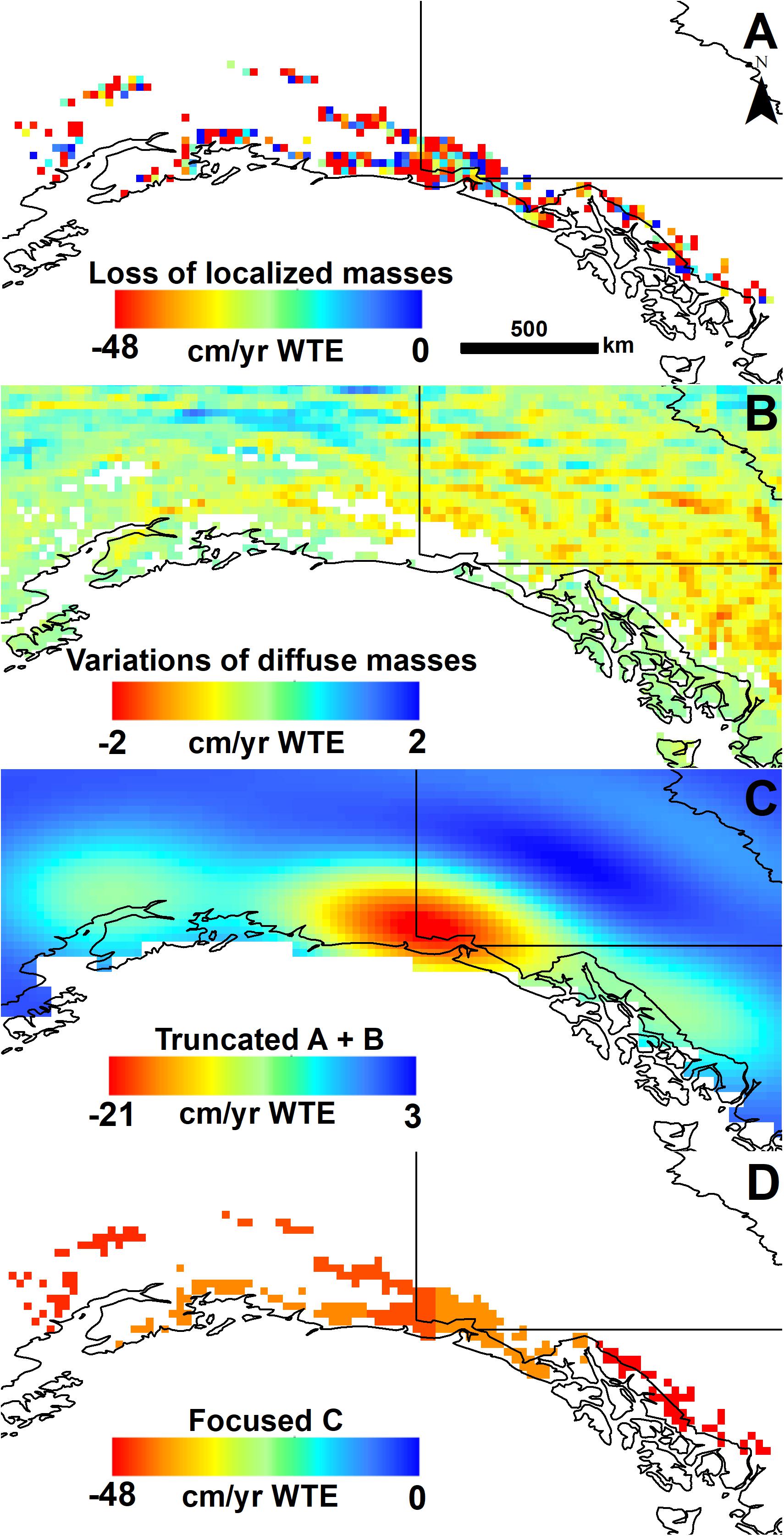
Figure 3. (A) Synthetic mass randomly allocated to pixels corresponding to glaciers. (B) Soil moisture trend from GLDAS Noah Land Surface Model (LSM) v2.1. (C) Forward model (FM) of A overlaid on B, representing a realistic reproduction of the GRACE trend signal derived from known masses. It includes both concentrated and diffuse mass changes in realistic proportions. (D) Example of a high resolution glacier mass loss map retrieved by applying the inversion procedure over C and using the 5-mascon delineation shown in Figure 2A. This synthetic test allows to assess the inversion procedure and its ability to retrieve glacier mass losses at high resolution. Results are presented in Supplementary Table S1.

TABLE 3

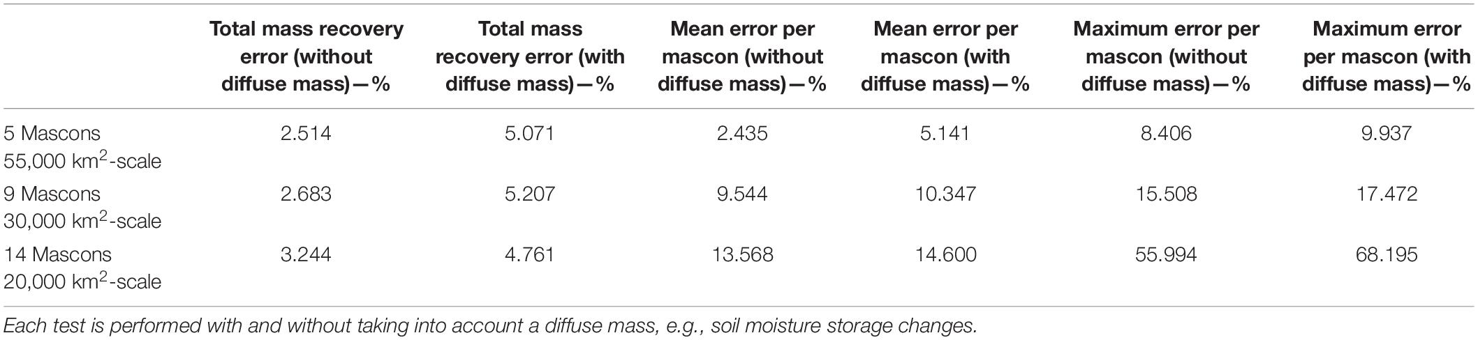
Table 3. Errors in recovering known synthetic masses allocated over the distribution map (Figure 3).

We observe that the total mass is well recovered regardless of the number of mascons and of the consideration of a diffuse mass during the inversion (Table 3). The Mean Absolute Relative Error (MARE) of the mass recovery at the mascon resolution ranges from ∼5 to ∼15%, and increases with the resolution of the mascon map. The maximum error goes up to ∼68% while recovering masses over small mascons (14-mascon delineation). We conclude that an acceptable accuracy is obtained while using mascon size up to ∼30,000 km².

The differences observed in the total mass recovery, considering or not a diffuse mass, are less than 3% for the three mascon delineations. The maximum additional error related to the inclusion of a diffuse mass is ∼2% for the 5 and 9-mascon delineations and reaches ∼12% for the 14-mascon delineation. This suggests that the inclusion of a supplementary mascon expected to account for diffuse masses (low-frequency signals) did not help to recover the glacial masses. This result, along with observations from the literature (e.g., Jin et al., 2017), and the apparently strong TWS trend (Figure 3), supports the common assumption that GRACE TWS signal is largely dominated by glacier ice mass changes in the GOA. It also suggests that the inversion performed with the actual GRACE TWS data does not need to consider a diffuse mass.

GOA-Scale Ice Mass Loss

GRACE TWS signal over the GOA shows a negative anomaly in all three solutions (Figure 4). They are all showing a very similar mass depletion across the GOA, in both amplitude and spatial extent (Figures 4A–C). The GRGS solution shows a slightly different spatial pattern at the eastern tip of the anomaly. Given that all solutions were corrected for GIA using the same model (Geruo et al., 2013) and that all solutions were at the same resolution (SH coefficients up to degree/order 90), the most likely reason for the perceptible differences is related to the de-striping strategy, which is different for all the three solutions considered.

FIGURE 4

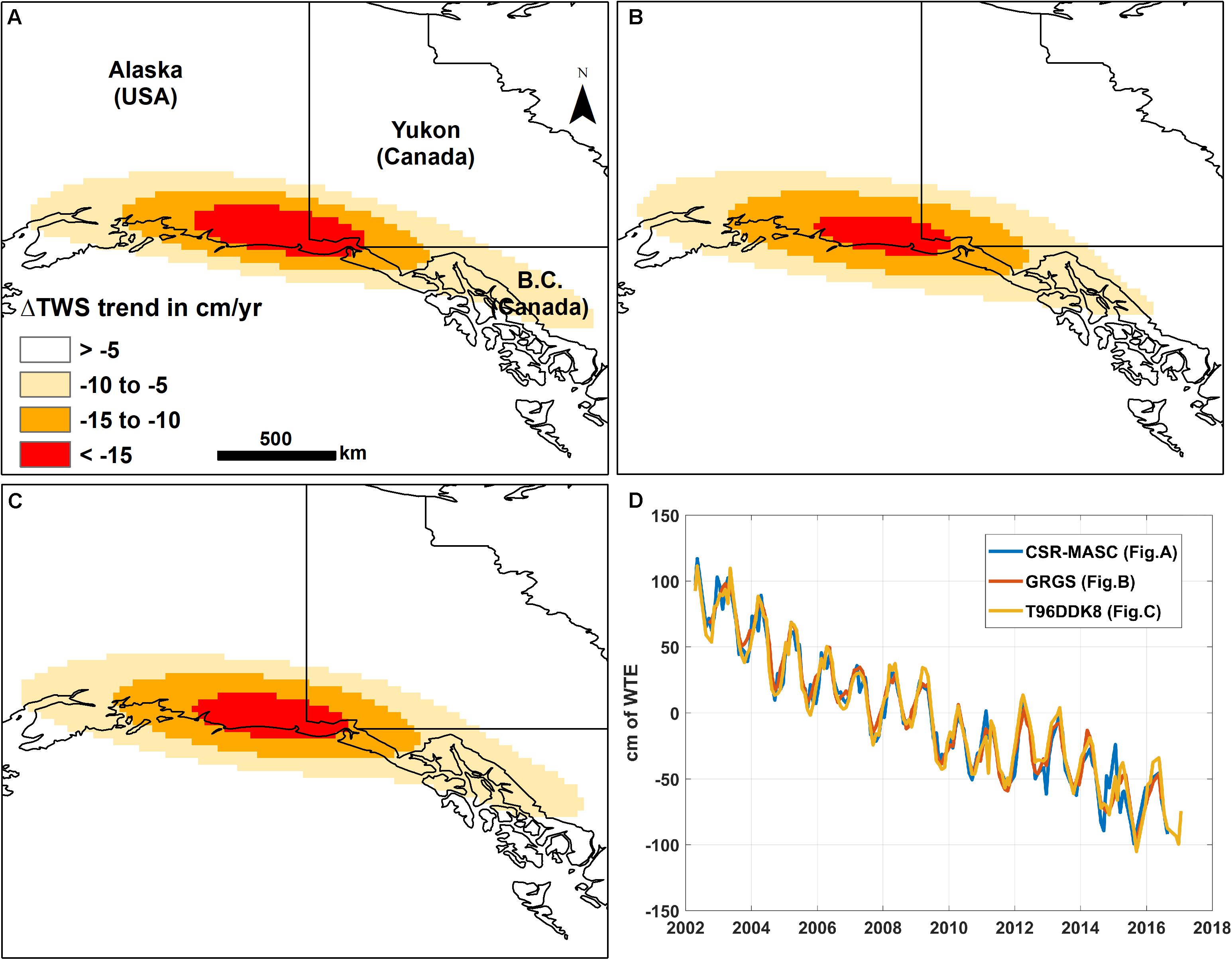
Figure 4. TWS signal trend over the study area using the three GRACE solutions: (A) CSR-MASC, (B) GRGS, (C) T96DDK8, and (D) near-monthly time-series of TWS change in WTE for the period 2012–2017 observed at the center of the anomaly.

The total mass loss rates were recovered by distributing mass loss values in each mascon until the FM reaches a minimum residual when subtracted from the GRACE TWS of each solution. Results are generally consistent regardless of the distribution considered (Table 4).

TABLE 4

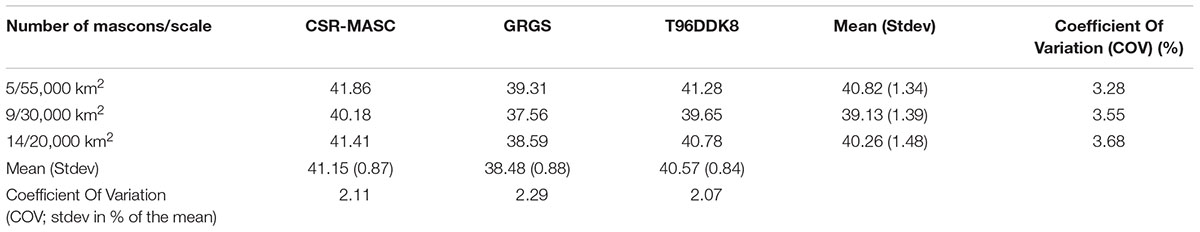
Table 4. Total mass loss estimated using to the three GRACE TWS solutions and the three mascon delineations in Gt/year (Figure 2).

The test with synthetic data shows that the error in recovering the total mass is ∼5% regardless of the mascon resolution. On the one hand, using different solutions over the same distribution leads to a Coefficient Of Variation (COV) of ∼3.5% (Table 4). On the other hand, using different distributions with the same solution leads to a COV of ∼2.1%. The similarity between the solutions (Figure 4D and Table 4) proves a clear improvement in GRACE processing with the latest solutions from the 2016–2018 era such as CSR RL06. When considering an ample TWS anomaly like the GOA, solutions are usually leading to similar observations. However, it might not be the case when considering low amplitude signals which are closer to the noise level, and more sensitive to the processing strategy.

These results are compared with results from previous studies performed over the same area in Table 1. Jacob et al. (2012); Baur et al. (2013), and Wahr et al. (2016) found ice loss rates within the range 47–52 Gt/year, which is in good agreement with our results (Figure 5). Tamisiea et al. (2005); Chen et al. (2006), and Luthcke et al. (2008) found significantly higher ice loss rates. This can be related to the shorter TWS time-series and the larger uncertainties associated with the early releases of GRACE TWS data. Our results are close to the estimates from studies using different methods (Berthier et al., 2010; Gardner et al., 2013; Larsen et al., 2015, values are listed in section “Introduction”).

FIGURE 5

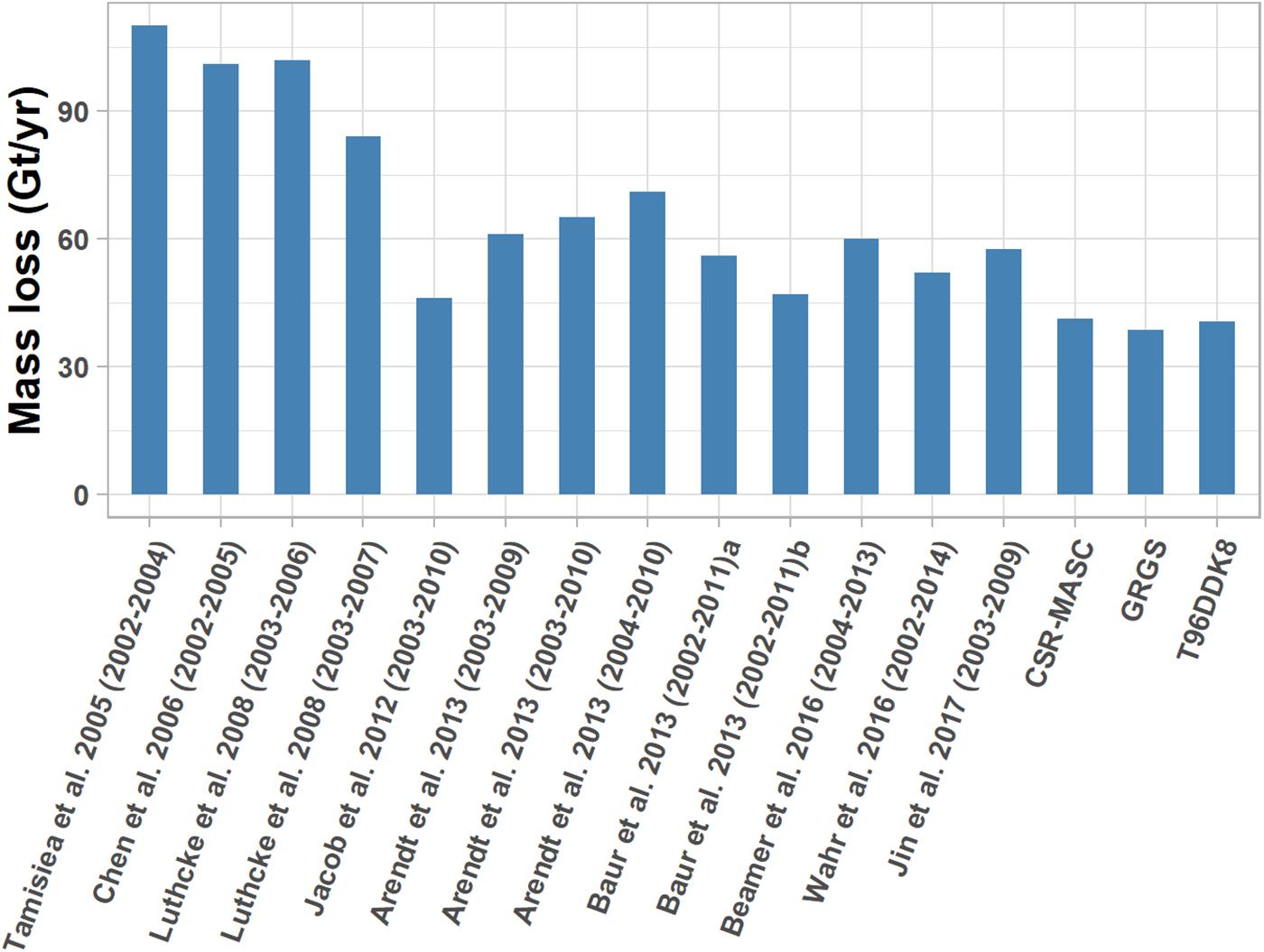
Figure 5. Comparison between glacier mass loss estimates from this study with those of other studies listed in Table 1.

Differences in GRACE Level-3 data interpretation strategy can lead to discrepancies with estimates from other authors. The use of a constrained forward modeling strategy can lead to lower values, as it only recovers the signal spatially correlated to glaciers (see, e.g., Long et al., 2016, for an example related to groundwater depletion). The injection of a distribution constraint is known to reduce contributions from unwanted signals with contrasting spatial patterns. These signals cannot be focused onto the constraining distribution (Farinotti et al., 2015; Castellazzi et al., 2018). However, the distribution map is a simplification of the reality as it does not consider the intra-mascon heterogeneity of the ice loss signal. This might lead to uncertainties, depending on the level of unaccounted heterogeneity and its location on the distribution map.

Mascon-Scale Ice Mass Loss

In this section, we discuss the reliability of considering mass losses focused over mascon at different scales. For each inversion, the result corresponds to the best fit to reproduce the true GRACE TWS over the GOA. Total per-mascon masses are presented in Table 5, and the spatial patterns of the mean and standard deviation of glacier mass changes are shown in Figure 6. As discussed previously, we assume that the degree of similarity between the mass losses retrieved using the three solutions represents a good indicator of accuracy. The maximum value of variation within each mascon corresponds to ∼13, ∼25, and ∼40% of the mean mass allocated, for the 5-, 9-, and 14-mascon delineations, respectively. It is observed that this variation tends to increase over the East/West extremes of the study area (Table 6 and Figure 6). This corresponds to differences observed by comparing the low resolution GRACE TWS trend maps (Figure 4) which propagates into the inversion results. These variations due to differences in processing strategies increase with the spatial resolution (Table 6); hence the estimates for the 14-mascon delineation have the highest level of uncertainty.

TABLE 5

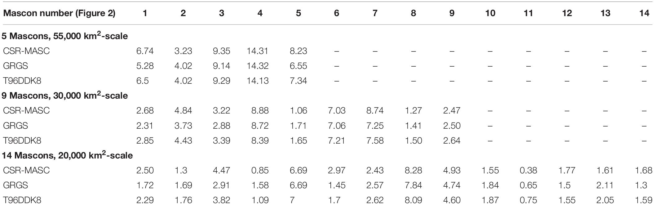
Table 5. Mass losses measured in each mascon in Gt/year.

FIGURE 6

Figure 6. High resolution mapping according to the three mass distribution scenarios (Figure 2): mean mass loss (A–C) and standard deviation (D–F). Maps are presented in order of focusing resolution: (A–D) 5-, (B–E) 9-, and (C–F) 14-mascon delineations. Two different scales of the same color maps are used for A–C and D–F.

TABLE 6

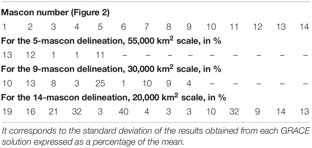
Table 6. Coefficient Of Variation (COV) of the focused masses.

We evaluate the accuracy of our mass loss estimates by comparison with those from other studies. This comparison is based on the area with the largest mass losses, which are the Saint Elias Mountains and Glacier Bay, according to Luthcke et al. (2013). This was confirmed by Arendt et al. (2013), who showed that the Saint Elias Mountains, Glacier Bay, and Juneau icefield regions present the largest amount of glacier mass losses. Jin et al. (2017) indicated that the Malaspina and Bering glaciers, belonging to the Saint Elias Mountains, have the largest rates of ice mass losses. Glaciers of the Saint Elias Mountains correspond to mascons 6, 7, and 10 in Luthcke et al. (2008; see Figure 7A) and mascon 6 in Arendt et al. (2013; see Figure 7B). Our estimates agree with the aforementioned studies which indicate that glaciers of the Saint Elias Mountains have the largest mass loss rates in the region (see Supplementary Tables S2, S3).

FIGURE 7

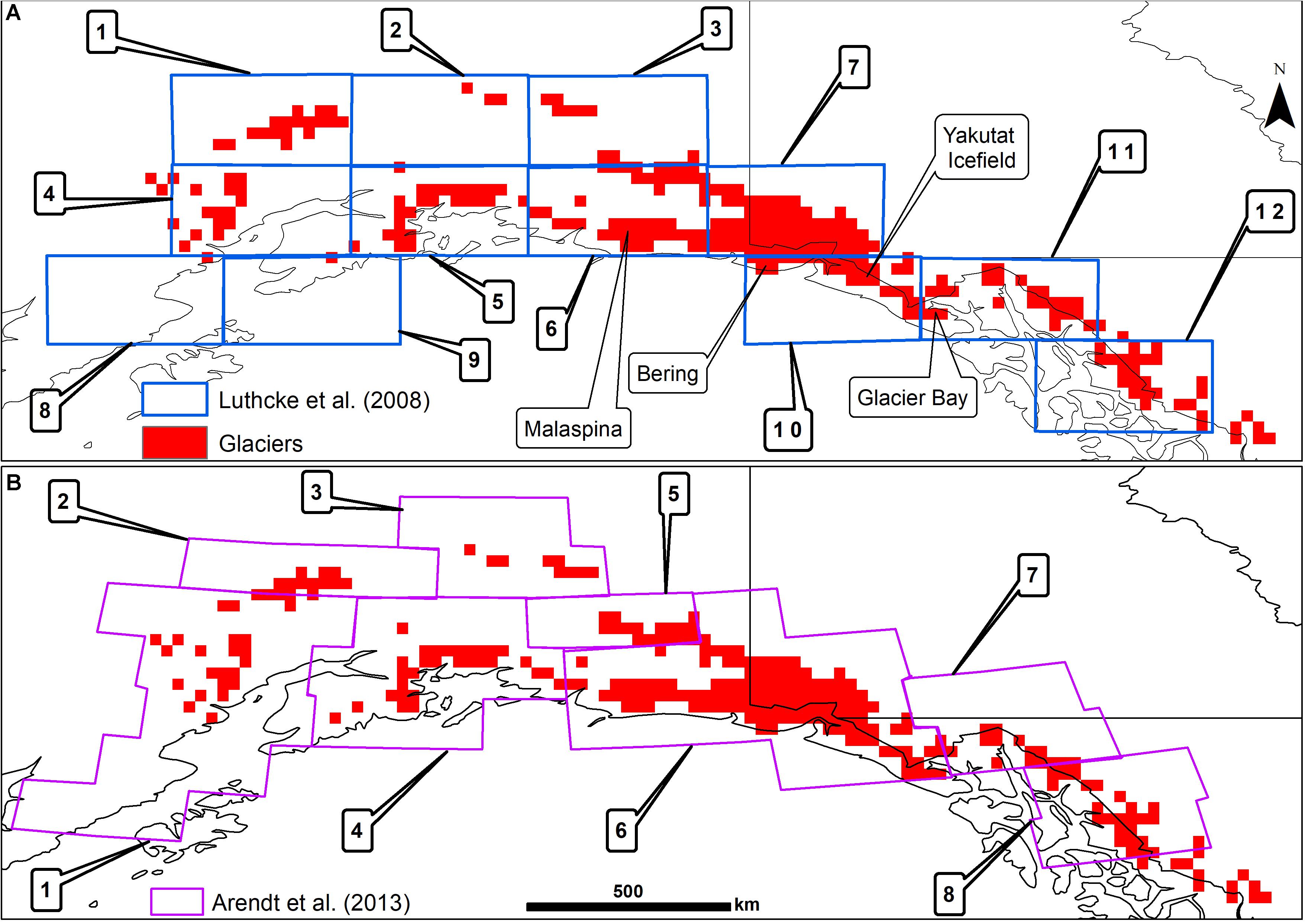
Figure 7. Overlay of mascon delineations from other studies over the glacier distribution map used in this study: (A) delineation used by Luthcke et al. (2008) and (B) delineation used by Arendt et al. (2013), in which Glacier Bay is included in mascon 6, corresponding to the Saint Elias Mountains (Supplementary Table S2).

Arendt et al. (2008) used the same delineation and GRACE TWS solution as Luthcke et al. (2008; see Figure 7A). By down-sampling the solution to the Saint Elias Mountains (cumulating rates from mascons 6, 7, and 10; Figure 7A in Luthcke et al., 2008), using the ratio of ice area in each mascon over the period 2003–2007, they obtained 20.6 ± 3.0 Gt/year of ice loss. Luthcke et al. (2008) calculated 36 ± 2.0 and 30 ± 2.0 Gt/year of ice mass loss by using GRACE data for 2003–2006 and 2003–2007, respectively. First, we compare the results from these two studies with our estimates over the period 2002–2017 (Table 7), and we create a temporal subset from our estimates to make our comparison insensitive to discordances in the time-period considered.

TABLE 7

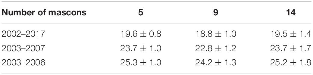
Table 7. Mean mass losses in Gt/year considering three different time-periods over a spatial subset corresponding to mascons 6, 7, and 10 in Luthcke et al. (2008; see Figure 7A), which correspond to the Saint Elias Mountains.

Comparing our results with two other studies (Arendt et al., 2008; Luthcke et al., 2008) after applying similar spatial constraints, we observe that the results from Arendt et al. (2008) are similar to our estimates regardless of the mascon delineation considered. Results from Luthcke et al. (2008) are generally larger than our estimates, as do most other studies using GRACE data from the 2003–2006 time-period. However, we note similarities for mascon numbers 5, 6, and 7, at the center of the GOA, where the mass change is the strongest (Supplementary Table S3). This observation coincides with our visual observation of the spatial patterns of mass losses (Table 6). It points out that the weaker signal at the extreme East-West side is sensitive to the processing strategy and its corresponding residual noise pattern.

Considering the ice loss rates over the same time-period allows us to understand the source of the differences observed between our results and these two studies. To do so, we calculated the ratios between the trend at the center of the Saint Elias Mountains derived from the full length of the GRACE time-series and the trend computed after selecting a temporal subset corresponding to the time scale of their study (Supplementary Figure S2). All the trends have been determined by using the method described in Supplementary Figure S1. We then reported the ratios obtained over the trend rates from our focused trend maps. The results from our study over these short periods (i.e., 2003–2006 and 2003–2007) are ∼20% larger than those over the period 2002–2017 (Table 7). We conclude that the use of a shorter time-series plays a significant role in the differences observed with results from other studies, and that these differences may not only be due to the choice of GRACE processing strategy. In other words, estimations built from a short GRACE times-series (3–4 years from 2003) have overestimated the long-term glacial mass loss by ∼20%. The inter-annual variability of the snow cover might strongly influence the TWS while considering short time-series.

We also compared our results over the Saint Elias Mountain with the mascon solution from NASA GSFC (v2.4; Luthcke et al., 2013; see Supplementary Figure S3), which considers GRACE data from 2003 to 2016. The mass loss rate obtained by using this dataset over the Saint Elias Mountains is 24.85 ± 2.1 Gt/year. Over the same area, we estimate the glacial mass loss at 22.01 ± 0.89, 21.57 ± 1.18, and 21.41 ± 1.64 Gt/year for our three mascon resolutions. Our results are very close to those from the NASA GSFC mascon data (v02.4), and the slight difference might be attributed to the difference in time-series length (2003–2016 versus 2002–2017).

Inversion Residuals

Residual maps are produced by subtracting the FM of the high resolution mass distribution maps from the actual GRACE TWS signal. The amplitude of the residual decreases with the mascon extent. This confirms the ability to retrieve the total mass when a large number of mascons are used. However, as previously discussed, it is at the cost of a lower accuracy at the mascon scale.

We note that the inversion residuals from the GRGS and T96DDK8 solutions have similar spatial patterns. It is negligible inland (values below ± 2 cm/year) and more important near the ocean (close to −5 cm/year). The high absolute residual value near the ocean could be due to coastal glaciers covered by the land mask, implying that a part of the signal from these glaciers is not recovered through the focusing procedure.

Following Wahr et al. (2006) and Ramillien et al. (2017), the GRACE TWS data contain noise patterns from measurements and processing errors. We compare the amplitude of the noise with the residuals of the inversion procedure to verify the performance of the inversion (Figure 8). We consider that the noise level can be approximated by observing the maximum amplitude of mass trends in the Pacific Ocean at similar latitudes than our study area. We found values of ∼1.4, 1.6, and 1.5 cm/year for the CSR-MASC, GRGS, and T96DDK8 solutions, respectively. These values are close to the residuals (values between [−2: +2] cm/year), which suggests that the remaining signal left after mass concentration might not be attributed to the glacial mass loss.

FIGURE 8

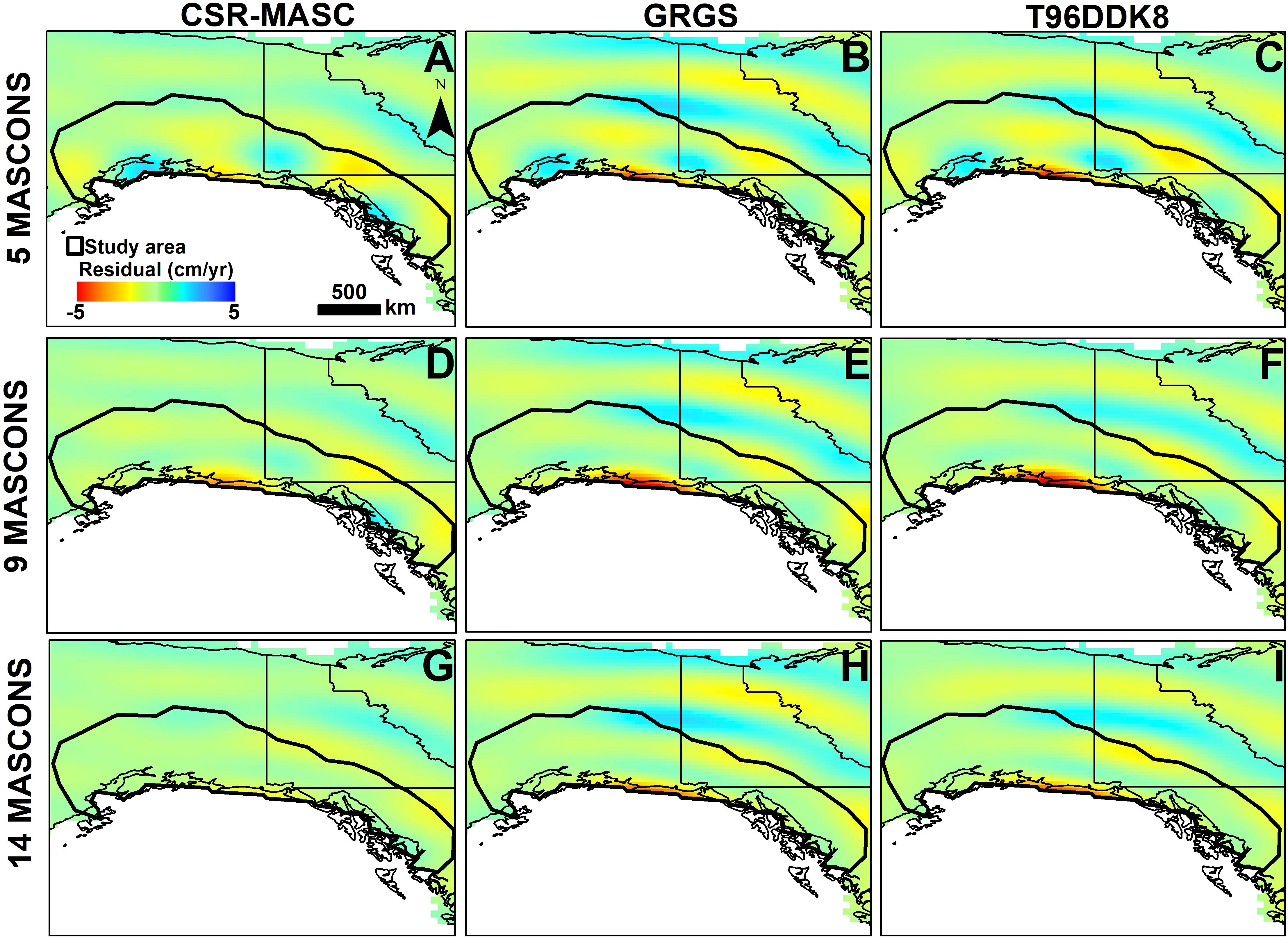
Figure 8. Residual maps of the focusing procedure in WTE. These maps represent the signal remaining after subtracting the best forward model (FM) to the actual GRACE TWS signal. The labels showed in (A) correspond to all of the residuals (A–I). According to these labels, the negative values of Mass loss, in cm/year, indicate that the estimates from GRACE solutions are higher than those from the forward model. The positive values show that the Mass loss from the forward model is higher.

Conclusion

This study shows a downscaling approach of GRACE TWS data which can be used to retrieve a high resolution ice mass loss. We tested three GRACE solutions and three uniform focusing delineations, and applied an inversion method which relies on fitting iteratively a spatially constrained FM. We used the three solutions at the same truncation level (resolution) in order to isolate the effect of the processing strategy applied to the GRACE data from Level 1 to 3. From our study, we can draw three key findings.

First, synthetic simulations indicate that the forward modeling approach is efficient, with a mean error of ∼2.5% when considering the total mass loss over the GOA, and below 10% when considering masses at the mascon-scale and with mascons up to 30,000 km². It also shows that our inversion procedure is relatively insensitive to non-ice masses such as soil moisture.

Second, at the scale of the GOA, the resolution of the mass concentration units (referred to as mascon) and the choice of the GRACE solution strategy only account for an uncertainty of ∼2–4% in the total mass estimation. The three solutions provide approximatively the same total mass loss (∼40 Gt/year) over the era 2002–2017.

Third, at the scale of a mascon of 30,000 km² or larger, the focusing procedure recovers well the regional mass loss signal. At this scale, the mascon contain from 1 to 9 Gt/year of ice mass loss, the highest mass loss rates being at the center of the area, over the Saint Elias Mountains. Variations between solutions reach 40% of the mean signal when considering high resolution mascons of 20,000 km². Residuals are of the same order of magnitude as the noise level of GRACE TWS solutions. Thus, the glacier signals are well retrieved when using an inversion with a uniform constrained FM, and the distribution map is efficient at concentrating the mass loss observed by GRACE.

We compared our results with estimates reported in the literature and found a good agreement with studies using GRACE solutions from recent releases and time-series of more than 8 years. The first studies using GRACE data published during the 2005–2008 era generally overestimated the long-term ice mass loss at the GOA scale due to the data time-span, the interpretation strategy, and possibly the use of early release of GRACE data. Comparing our ice loss map at the highest resolution with those of Arendt et al. (2008) and the mascon solution from NASA GSFC over the Saint Elias Mountains, we obtained relatively similar ice loss rates. This area of comparison is at the center of the GOA, where our results are the most reliable, with mass losses and signal–noise ratio at the highest.

To our knowledge, this is the first study presenting a focused and spatially constrained ice loss map over the GOA. Comparison of our findings with results from other data sources (i.e., altimetry) could help further assessing the accuracy of our estimates. Constraining the focusing procedure using a heterogeneous mass loss map from other data sources would allow to cope with the heterogeneity of the losses, which is partially unaccounted for in this study. The findings of this study could help integrating an ice mass loss module into large-scale hydrological models; providing a framework to better understand the effect of climate change on the hydrological cycle of the main river basins of the GOA area.

Data Availability Statement

We provided in the article/Supplementary Material the links and the references to access all datasets used for this study.

Author Contributions

CD performed the data analysis and wrote the manuscript. PC trained the first author to process GRACE data, verified the results, and contributed to the writing of the manuscript. AR designed and led the project, supervised CD, and contributed to the writing of the manuscript. MA helped to build a comprehensive literature review on the topic.

Funding

The authors wish to gratefully acknowledge the financial support of the Natural Sciences and Engineering Research Council of Canada (NSERC) and the Yukon Energy Corporation (YEC) for this research.

Conflict of Interest

The authors declare that the research was conducted in the absence of any commercial or financial relationships that could be construed as a potential conflict of interest.

Acknowledgments

The authors would like to thank Wei Feng (Chinese Academy of Sciences) for the development of GRAMAT (GRACE Matlab Toolbox) (MATLAB and Statistics Toolbox Release 2017a, The MathWorks, Inc., Natick, MA, United States) which was used to process GRACE data.

Supplementary Material

The Supplementary Material for this article can be found online at: https://www.frontiersin.org/articles/10.3389/feart.2019.00360/full#supplementary-material

Footnotes

1. ^ http://nsidc.org/glims/
2. ^ http://grgs.obs-mip.fr/grace

References

Arendt, A., Luthcke, S., Gardner, A., O’Neel, S., Hill, D., Moholdt, G., et al. (2013). Analysis of a GRACE global mascon solution for Gulf of Alaska glaciers. J. Glacio. 59, 913–924. doi: 10.3189/2013JoG12J197

CrossRef Full Text | Google Scholar

Arendt, A. A., Luthcke, S. B., and Hock, R. (2009). Glacier changes in Alaska: can mass-balance models explain GRACE mascon trends? Ann. Glaciol. 50, 148–154. doi: 10.3189/172756409787769753

CrossRef Full Text | Google Scholar

Arendt, A. A., Luthcke, S. B., Larsen, C. F., Abdalati, W., Krabill, W. B., and Beedle, M. J. (2008). Validation of high-resolution GRACE mascon estimates of glacier mass changes in the St Elias Mountains, Alaska, USA, using aircraft laser altimetry. J. Glaciol. 54, 778–787. doi: 10.3189/002214308787780067

CrossRef Full Text | Google Scholar

Baur, O., Kuhn, M., and Featherstone, W. E. (2013). Continental mass change from GRACE over 2002–2011 and its impact on sea level. J. Geodesy 87, 117–125. doi: 10.1007/s00190-012-0583-2

CrossRef Full Text | Google Scholar

Beamer, J. P., Hill, D. F., Arendt, A., and Liston, G. E. (2016). High-resolution modeling of coastal freshwater discharge and glacier mass balance in the Gulf of Alaska watershed: coastal fwd and gvl in goa watershed. Water Resour. Res. 52, 3888–3909. doi: 10.1002/2015WR018457

CrossRef Full Text | Google Scholar

Berthier, E., Schiefer, E., Clarke, G. K. C., Menounos, B., and Rémy, F. (2010). Contribution of Alaskan glaciers to sea-level rise derived from satellite imagery. Nat. Geosci. 3, 92–95. doi: 10.1038/ngeo737

CrossRef Full Text | Google Scholar

Blanchon, D., and Boissière, A. (2009). Atlas Mondial de l’eau: De l’eau Pour Tous. Paris: Autrement.

Google Scholar

Castellazzi, P., Burgess, D., Rivera, A., Huang, J., Longuevergne, L., and Demuth, M. N. (2019). Glacial melt and potential impacts on water resources in the Canadian Rocky Mountains. Water Resour. Res. 55. doi: 10.1029/2018WR024295

CrossRef Full Text | Google Scholar

Castellazzi, P., Longuevergne, L., Martel, R., Rivera, A., Brouard, C., and Chaussard, E. (2018). Quantitative mapping of groundwater depletion at the water management scale using a combined GRACE/InSAR approach. Remote Sens. Environ. 205, 408–418. doi: 10.1016/j.rse.2017.11.025

CrossRef Full Text | Google Scholar

Castellazzi, P., Martel, R., Rivera, A., Huang, J., Pavlic, G., Calderhead, A. I., et al. (2016). Groundwater depletion in Central Mexico: use of GRACE and InSAR to support water resources management. Water Resour. Res. 52, 5985–6003. doi: 10.1002/2015WR018211

CrossRef Full Text | Google Scholar

Chen, J., and Ohmura, A. (1990). “Estimation of Alpine glacier water resources and their change since the 1870s,” in Proceedings of the IAHS (Symopsium at Lausanne, 1990 – Hydrology in Mountainous Regions I), (Wallingford: IAHS), 127–135.

Google Scholar

Chen, J. L., Tapley, B. D., and Wilson, C. R. (2006). Alaskan mountain glacial melting observed by satellite gravimetry. Earth Planet. Sci. Lett. 248, 368–378. doi: 10.1016/j.epsl.2006.05.039

CrossRef Full Text | Google Scholar

Chen, J. L., Wilson, C. R., Blankenship, D., and Tapley, B. D. (2009). Accelerated Antarctic ice loss from satellite gravity measurements. Nat. Geosci. 2, 859–862. doi: 10.1038/ngeo694

CrossRef Full Text | Google Scholar

Chen, J. L., Wilson, C. R., Li, J., and Zhang, Z. (2015). Reducing leakage error in GRACE-observed long-term ice mass change: a case study in West Antarctica. J. Geodesy 89, 925–940. doi: 10.1007/s00190-015-0824-2

CrossRef Full Text | Google Scholar

Farinotti, D., Longuevergne, L., Moholdt, G., Duethmann, D., Mölg, T., Bolch, T., et al. (2015). Substantial glacier mass loss in the Tien Shan over the past 50 years. Nat. Geosci. 8, 716–722. doi: 10.1038/ngeo2513

CrossRef Full Text | Google Scholar

Frans, C., Istanbulluoglu, E., Lettenmaier, D. P., Fountain, A. G., and Riedel, J. (2018). Glacier recession and the response of summer streamflow in the Pacific Northwest United States, 1960-2099. Water Resour. Res. 54, 6202–6225. doi: 10.1029/2017WR021764

CrossRef Full Text | Google Scholar

Gardner, A. S., Moholdt, G., Cogley, J. G., Wouters, B., Arendt, A. A., Wahr, J., et al. (2013). A reconciled estimate of glacier contributions to sea level rise: 2003 to 2009. Science 340, 6134–6152. doi: 10.1126/science.1234532

PubMed Abstract | CrossRef Full Text | Google Scholar

Geruo, A., Wahr, J., and Zhong, S. (2013). Computations of the viscoelastic response of a 3-D compressible Earth to surface loading: an application to glacial isostatic adjustment in Antarctica and Canada. Geophys. J. Int. 192, 557–572. doi: 10.1093/gji/ggs030

CrossRef Full Text | Google Scholar

GLIMS and NSIDC (2005, updated in 2013). Global Land Ice Measurements from Space Glacier Database. Compiled and made available by the international GLIMS community and the National Snow and Ice Data Center. Boulder, CO: National Snow and Ice Data Center.

Google Scholar

Hingray, B., Picouet, C., and Musy, A. (2014). Hydrologie 2 Une Science Pour l’ingénieur, 1ère édition. Palawan: PPUR.

Google Scholar

Hock, R. (1999). A distributed temperature index ice and snow melt model including potential direct solar radiation. J. Glaciol. 45, 101–111. doi: 10.3189/S0022143000003087

CrossRef Full Text | Google Scholar

Hooke, R., and Jeeves, T. A. (1961). “Direct search” solution of numerical and statistical problems. J. ACM 8, 212–229. doi: 10.1145/321062.321069

CrossRef Full Text | Google Scholar

Huss, M., and Hock, R. (2018). Global-scale hydrological response to future glacier mass loss. Nat. Clim. Change 8, 135–140. doi: 10.1038/s41558-017-0049-x

CrossRef Full Text | Google Scholar

Jacob, T., Wahr, J., Pfeffer, W. T., and Swenson, S. (2012). Recent contributions of glaciers and ice caps to sea level rise. Nature 482, 514–518. doi: 10.1038/nature10847

PubMed Abstract | CrossRef Full Text | Google Scholar

Jin, S., and Feng, G. (2016). Uncertainty of Grace-Estimated Land Water and Glaciers Contributions to Sea Level Change During 2003–2012 (Beijing: IEEE), 6189–6192. doi: 10.1109/IGARSS.2016.7730617

CrossRef Full Text | Google Scholar

Jin, S., Zhang, T. Y., and Zou, F. (2017). Glacial density and GIA in Alaska estimated from ICESat, GPS and GRACE measurements: glacial density and GIA in Alaska. J. Geophys. Res. Earth Surf. 122, 76–90. doi: 10.1002/2016JF003926

CrossRef Full Text | Google Scholar

Jin, S., and Zou, F. (2015). Re-estimation of glacier mass loss in Greenland from GRACE with correction of land–ocean leakage effects. Glob. Planet. Change 135, 170–178. doi: 10.1016/j.gloplacha.2015.11.002

CrossRef Full Text | Google Scholar

Kienholz, C., Herreid, S., Rich, J. L., Arendt, A. A., Hock, R., and Burgess, E. W. (2015). Derivation and analysis of a complete modern-date glacier inventory for Alaska and northwest Canada. J. Glaciol. 61, 403–420. doi: 10.3189/2015JoG14J230

CrossRef Full Text | Google Scholar

Kolda, T. G., Lewis, R. M., and Torczon, V. (2003). Optimization by direct search: new perspectives on some classical and modern methods. SIAM Rev. 45, 385–482. doi: 10.1137/S003614450242889

CrossRef Full Text | Google Scholar

Kusche, J. (2007). Approximate decorrelation and non-isotropic smoothing of time-variable GRACE-type gravity field models. J. Geodesy 81, 733–749. doi: 10.1007/s00190-007-0143-3

CrossRef Full Text | Google Scholar

Kusche, J., Schmidt, R., Petrovic, S., and Rietbroek, R. (2009). Decorrelated GRACE time-variable gravity solutions by GFZ, and their validation using a hydrological model. J. Geodesy 83, 903–913. doi: 10.1007/s00190-009-0308-3

CrossRef Full Text | Google Scholar

Larsen, C. F., Burgess, A., Arendt, A., O’Neel, S., Johnson, A. J., and Kienholz, C. (2015). Surface melt dominates Alaskaglacier mass balance. Geophys. Res. Lett. 42, 5902–5908. doi: 10.1002/2015GL064349

CrossRef Full Text | Google Scholar

Larsen, C. F., Motyka, R. J., Arendt, A. A., Echelmeyer, K. A., and Geissler, P. E. (2007). Glacier changes in southeast Alaska and northwest British Columbia and contribution to sea level rise. J. Geophys. Res. 112:F01007. doi: 10.1029/2006JF000586

CrossRef Full Text | Google Scholar

Long, D., Chen, X., Scanlon, B. R., Wada, Y., Hong, Y., Singh, V. P., et al. (2016). Have GRACE satellites overestimated groundwater depletion in the Northwest India Aquifer? Sci. Rep. 6:24398. doi: 10.1038/srep24398

PubMed Abstract | CrossRef Full Text | Google Scholar

Longuevergne, L., Scanlon, B. R., and Wilson, C. R. (2010). GRACE hydrological estimates for small basins: evaluating processing approaches on the High Plains Aquifer, USA: grace hydrological estimates for small b. Water Resour. Res. 46:W11517. doi: 10.1029/2009WR008564

CrossRef Full Text | Google Scholar

Luthcke, S. B., Arendt, A. A., Rowlands, D. D., McCarthy, J. J., and Larsen, C. F. (2008). Recent glacier mass changes in the Gulf of Alaska region from GRACE mascon solutions. J. Glaciol. 54, 767–777. doi: 10.3189/002214308787779933

CrossRef Full Text | Google Scholar

Luthcke, S. B., Sabaka, T. J., Loomis, B. D., Arendt, A. A., McCarthy, J. J., and Camp, J. (2013). Antarctica, Greenland and Gulf of Alaska land-ice evolution from an iterated GRACE global mascon solution. J. Glaciol. 59, 613–631. doi: 10.3189/2013JoG12J147

CrossRef Full Text | Google Scholar

Pfeffer, W. T., Arendt, A. A., Bliss, A., Bolch, T., Cogley, J. G., Gardner, A. S., et al. (2014). The Randolph Glacier Inventory: a globally complete inventory of glaciers. J. Glaciol. 60, 537–552. doi: 10.3189/2014JoG13J176

CrossRef Full Text | Google Scholar

Pomeroy, J. W., Gray, D. M., Brown, T., Hedstrom, N. R., Quinton, W. R., Granger, R. J., et al. (2007). The cold regions hydrological model: a platform for basing process representation and model structure on physical evidence. Hydrol. Process. 21, 2650–2667. doi: 10.1002/hyp.6787

CrossRef Full Text | Google Scholar

Radić, V., and Hock, R. (2011). Regionally differentiated contribution of mountain glaciers and ice caps to future sea-level rise. Nat. Geosci. 4, 91–94. doi: 10.1038/ngeo1052

CrossRef Full Text | Google Scholar

Ramillien, G., Frappart, F., and Seoane, L. (2017). “La mission de gravimétrie spatiale GRACE: instruments et principe de fonctionnement,” in Observations Des Surfaces Continentales par Télédétection Micro-Onde: Techniques et Méthodes, eds N. Baghdadi and M. Zribi, (London: ISTE), 281–297.

Google Scholar

Raup, B., Racoviteanu, A., Khalsa, S. J. S., Helm, C., Armstrong, R., and Arnaud, Y. (2007). The GLIMS geospatial glacier database: a new tool for studying glacier change. Glob. Planet. Change 56, 101–110. doi: 10.1016/j.gloplacha.2006.07.018

CrossRef Full Text | Google Scholar

Rodell, M., Houser, P. R., Jambor, U., Gottschalck, J., Mitchell, K., Meng, C.-J., et al. (2004). The global land data assimilation system. Bull. Am. Meteorol. Soc. 85, 381–394. doi: 10.1175/BAMS-85-3-381

CrossRef Full Text | Google Scholar

Save, H., Bettadpur, S., and Tapley, B. D. (2016). High-resolution CSR GRACE RL05 mascons: high-resolution CSR grace RL05 MASCONS. J. Geophys. Res. Solid Earth 121, 7547–7569. doi: 10.1002/2016JB013007

PubMed Abstract | CrossRef Full Text | Google Scholar

Tamisiea, M. E., Leuliette, E. W., Davis, J. L., and Mitrovica, J. X. (2005). Constraining hydrological and cryospheric mass flux in southeastern Alaska using space-based gravity measurements. Geophys. Res. Lett. 32:L20501. doi: 10.1029/2005GL023961

CrossRef Full Text | Google Scholar

Tapley, B. D., Bettadpur, S., Watkins, M., and Reigber, C. (2004). The gravity recovery and climate experiment: mission overview and early results: grace mission overview and early results. Geophys. Res. Lett. 31:4. doi: 10.1029/2004GL019920

CrossRef Full Text | Google Scholar

Wahr, J., Burgess, E., and Swenson, S. (2016). Using GRACE and climate model simulations to predict mass loss of Alaskan glaciers through 2100. J. Glaciol. 62, 623–639. doi: 10.1017/jog.2016.49

CrossRef Full Text | Google Scholar

Wahr, J., Molenaar, M., and Bryan, F. (1998). Time variability of the Earth’s gravity field: hydrological and oceanic effects and their possible detection using GRACE. J. Geophys. Res. Solid Earth 103, 30205–30229. doi: 10.1029/98JB02844

CrossRef Full Text | Google Scholar

Wahr, J., Swenson, S., and Velicogna, I. (2006). Accuracy of GRACE mass estimates. Geophys. Res. Lett. 33:L06401. doi: 10.1029/2005GL025305

CrossRef Full Text | Google Scholar

Yirdaw, S. Z., Snelgrove, K. R., Seglenieks, F. R., Agboma, C. O., and Soulis, E. D. (2009). Assessment of the WATCLASS hydrological model result of the Mackenzie River basin using the GRACE satellite total water storage measurement. Hydrol. Process. 23, 3391–3400. doi: 10.1002/hyp.7450

CrossRef Full Text | Google Scholar