Toward Reproducible Environmental Modeling for Decision Support: A Worked Example

1. Introduction

The importance of uncertainty quantification (UQ) in the context of environmental modeling for decision support is widely recognized (e.g., Anderson et al., 2015; Doherty, 2015a). So too is the importance of parameter estimation (PE), which, herein, we regard as the process of reducing uncertainty through history matching the simulation outputs to their state observation counterparts (a process often referred to as “calibration”). Together, UQ and PE represent critical analyses for model-based resource management decision support as they provide estimates of uncertainty in important simulated outcomes and reduce this uncertainty, respectively.

However, implementing high-dimensional UQ and PE in real-world modeling analyses can be difficult, from both a theoretical understanding standpoint (related to the depth and breadth of topical knowledge required), as well as from a mechanics/logistics standpoint arising from the preparation, implementation, and post-processing of these analyses. In the authors' experience, the difficulties commonly encountered when implementing UQ and PE for decision-support-scale modeling can preclude their application in many cases, especially when project time lines are short and funding is limited.

There are also strong calls for modeling based analysis (including UQ and PE analyses) to move toward more transparent, reproducible, and accountable processes. The reasons for this push are self-evident; several groups have called for increased transparency and reproducibility in computational science (Goecks et al., 2010; Stodden, 2010; Peng, 2011; Sandve et al., 2013; Liu et al., 2019) and in environmental simulation specifically Fienen and Bakker (2016). Some authors have put forward examples of increasing the reproducibility of the forward environmental model construction process (e.g., Fisher et al., 2016). To that end, some script-based tools have been developed for practitioners to increase the reproducibility of the forward model construction process (Olsthoorn, 2010; Fisher, 2014; Bakker et al., 2016). However, these tools are focused on the forward model rather than the UQ and PE process; in a decision-support setting, UQ and PE analyses are critical to the robust deployment of a model, and are therefore likely just as important as the forward model.

Ironically, the need for PE and UQ can be, in many contexts, in competition with the need for reproducibility. This is because the PE and UQ analyses require many additional subjective conceptual choices and bring many more operations and steps into the implementation of the modeling analysis, and these additional complications can substantially decrease the reproducibility of a modeling analyses. This decrease of reproducibility, especially in the outcomes of the PE and UQ analyses, can reduce the credibility of the model as a decision support tool and may hamper resource management efforts.

Herein, we present a step toward reproducible UQ and PE analysis through a script-based workflow. We use the term “reproducible” to mean giving readers access to the datasets and scripting tools needed to reproduce our results (e.g., figures, Supplementary Material and associated data release; White et al., 2020) and the findings based on them. Readers are referred to Plesser (2018) and Kitzes et al. (2017) (and the references cited therein) for a more nuanced and detailed discussion of what “reproducibility” means in the context of computational science.

Several open-source software tools were used to implement the UQ and PE workflow, including:

• The python package FloPy (Bakker et al., 2016) was used to programmatically load, process, and manipulate an existing groundwater flow model;

• The python package pyEMU (White et al., 2016) was used to programmatically construct a high-dimensional PEST interface (Doherty, 2015b) around the forward model and the generate the prior parameter ensembles;

• The iterative ensemble smoother PESTPP-IES (White, 2018) was used to evaluate the prior parameter ensembles (for UQ) and to also perform formal, high-dimensional PE.

Within this scripted workflow, we programmatically construct a high-dimensional truncated multi-variate (log-)Gaussian prior parameter distribution (hereinafter referred to as the “Prior”) and associated ensembles. The scripting is also used to define a subjective, management-focused likelihood function for the PE analysis. Additionally, we use scripting to post-process the results into the figures and Supplementary Material presented herein. In this way, we demonstrate that high-dimensional UQ and PE in real-world environmental modeling settings are achievable and can be both efficient and reproducible. Furthermore, given the increased interest in UQ and PE analyses in environmental simulation, the workflow presented herein provides the capability to efficiently and repeatably apply UQ and PE analyses to models that were previously constructed.

The rest of this manuscript is organized as follows. First, we briefly present the existing model, then we discuss the formulation of the Prior and the definition of the likelihood function used for PE, followed by the reproducible implementation and workflow presentation. Then the UQ and PE analysis results are presented, and finally, we discuss some nuances and implications of a script-driven UQ and PE workflow.

2. The Edwards Aquifer Model and Purpose of the Analysis

Herein, we use an existing model of the Edwards aquifer, Texas, USA from the work of Liu et al. (2017), based on the model of Lindgren et al. (2005). Briefly, the model is a MODFLOW-2005 (Harbaugh, 2005) model with 1 layer, 370 rows, and 700 columns arranged on a regular grid with a spacing of 1,340 feet; the geographic location of the model domain and features of interest are shown in Figure 1. Water enters the model domain as diffuse, areal recharge and as concentrated, stream-bed recharge—both of these recharge processes are simulated with the Recharge (RCH) package. Water leaves the model domain as spring flow (simulated with the Drain (DRN) package) and as extraction wells (simulated with the Well (WEL) package). Faults that are thought to function as barriers to flow are represented with the Horizontal Flow Barrier (HFB) package. Readers are referred to Liu et al. (2017) for more details regarding the model and specific simulations.

FIGURE 1

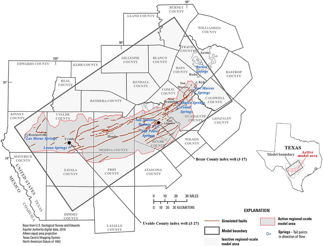
Figure 1. The geographic extent of the active model domain (gray) and locations of springs and groundwater-level observation locations of primary interest to groundwater resource managers. Modified from Brakefield et al. (2015).

The model has been temporally discretized into two simulation time periods:

• history-matching simulation: simulates the period 2001–2015 with monthly stress periods. This simulation is used for PE (i.e., history matching) of observed spring flows and groundwater levels;

• scenario simulation: simulates the period 1947–1958 (known as the “drought of record”) with monthly stress periods. This simulation is used to make a hindcast of simulated states of primary interest to groundwater resource managers, namely spring flow at Comal and San Marcos springs and groundwater level at index wells J-17 and J-27.

Both simulations use the same static (i.e., time-invariant) properties of hydraulic conductivity, storage, HFB conductances, and DRN boundary elements (stage and conductance). This is the mechanism for PE to reduce uncertainty in the scenario-simulation outputs of primary interest to groundwater resource managers. If these outputs are sensitive to the static properties and, through PE, the uncertainty in the static properties is reduced, then the uncertainty in the scenario-simulation outputs may also be reduced.

For the PE analysis, observations of spring flow and groundwater level are used for history matching from 6 and 336 locations, respectively, with a total of 1,060 spring flow state observations and 6,809 groundwater-level state observations.

2.1. Model Purpose

The flow from Comal and San Marcos springs and the groundwater levels at index wells J-17 and J-27 during the scenario (e.g., drought) simulation are of particular interest to groundwater resource management and are the primary focus of the UQ and PE analyses presented herein. Therefore, we focus the PE analysis on reproducing the observed spring flow and water levels listed above as robustly as possible during the history-matching simulation. Logically, reproducing these observed states during history-matching should improve the ability to simulate these observed states during the scenario simulation. We note that state observations of spring flow and groundwater level are also available for the scenario hindcast simulation at Comal and San Marcos springs and at index wells J-17 and J-27, respectively. However, we use these state observations only to verify the robustness (or otherwise) of the various workflow components, and, more generally, of the workflow itself; these scenario-period observations are not used for history-matching purposes.

2.2. Parameterization and the Prior

Herein, we use a Bayesian uncertainty framework (Tarantola, 2005) to represent uncertainty in parameters and outputs of primary interest to groundwater resource managers. A critical part of any Bayesian uncertainty quantification (UQ) analysis is definition of the Prior. We use a high-dimensional parameter space (Doherty et al., 2011) with the aim of achieving robust estimates for the hindcast of simulated states of primary interest to groundwater resource managers, while also attempting to avoid any ill-effects arising from under-parameterization (White et al., 2014; Knowling et al., 2019). Specifically, we used 337,482 and 339,449 parameters to represent model input uncertainty in the history-matching and scenario simulations, respectively (including the shared static property parameters, outlined above).

In the high-dimensional parameter space, we defined a truncated, multi-variate (log-)Gaussian distribution as the Prior; we used the existing history-matching and scenario simulation model inputs of Liu et al. (2017) as the first moment (e.g., mean vector) of the Prior and a block-diagonal covariance matrix for the second moment. Parameter variances were defined using expert knowledge and previous modeling analyses of the Edwards aquifer. The blocks in the prior parameter covariance matrix represent spatially- and temporally-correlated parameters, such as grid-scale and pilot-point (Doherty, 2003) parameters and time-varying parameters associated with well extraction rates. These correlations between spatially and temporally distributed parameters were specified using exponential variograms with the following ranges:

• 13,200 feet: grid-scale parameters, including hydraulic conductivity, specific storage, specific yield, initial conditions, HFB conductances; spatially-distributed well extraction rate parameters;

• 180 days: time-varying well extraction rate parameters; and

• 39,600 feet: pilot-point parameters, including hydraulic conductivity, specific storage, specific yield, initial conditions.

These ranges were selected so that the resulting spatially distributed model inputs had sufficient stochastic character in accordance with expert knowledge and previous modeling analyses of the Edwards aquifer.

Using the previously history-matched model inputs as the mean of the Prior is not standard practice in a purely Bayesian context because the same state observations will be used for conditioning herein. However, using the existing model inputs in this way allows us to take advantage of expert and institutional knowledge that has previously been assimilated into the model. Furthermore, using a very high-dimensional parameter space in combination with an ensemble framework allows us to account for the null-space contribution to uncertainty (Moore and Doherty, 2005) surrounding this history-matched location in parameter space.

We use a multi-scale parameterization strategy (McKenna et al., 2019) to explicitly represent different spatial scales of uncertainty and also to help understand how information is transferred from observed states to parameters (at different scales) in the PE analysis. For hydraulic conductivity, specific storage, specific yield, and initial conditions, three spatial scales of parameterization were used:

• a single, domain-wide (“global”) multiplier parameter;

• pilot point multiplier parameters (Doherty, 2003) at a spacing of 39,600 feet; and

• grid-scale multiplier parameters (one parameter per active computational cell).

Recharge was parameterized using time-varying domain-wide multiplier parameters in conjunction with time-varying multiplier parameters for each of the 25 unique recharge “zones”—for each stress period, a domain-wide multiplier parameter and a multiplier parameter for each zone was specified. In this way, we attempt to account for spatial uncertainty as well as temporal uncertainty in the recharge estimates. See Brakefield et al. (2015; Figure 15) for an example of the recharge zonation and Puente (1978) for a description of the Edwards aquifer recharge estimation process. Readers are referred to the Supplementary Material for a graphically summary of the multi-scale parameterization.

Well extraction rates were also parameterized to account for spatial and temporal uncertainty in the well extraction rate estimates. A single set of extraction rate multiplier parameters (one per well) was applied across all stress periods. This set of spatially distributed multiplier parameters were used with a set of temporally-distributed multiplier parameters (one for each stress period). We note that, while groundwater extraction rates were metered during the history-matching period, the simulated groundwater extraction in the model is nevertheless still uncertain as these metered rates may not capture all of the groundwater extraction that occurred and because of uncertainty (e.g., error) induced through spatial and temporal discretization.

Because the exact hydrologic disposition and function of the simulated HFBs is unknown, these were also parameterized at the grid scale. The conductance of each HFB cell was treated as uncertain but was spatially correlated with nearby HFB cells using a geostatistical variogram with a range of 13,200 feet.

A summary of the parameterization and prior parameter variances is presented in the Supplementary Material.

Note that separate temporal parameters (recharge, well extraction and initial conditions) are used for the history-matching and scenario simulations. All other parameters are shared between the two simulations.

2.3. The Likelihood

Given the intended management purposes(s) of this modeling analysis, we focused the PE analysis on reproducing the observed states from the history-matching period that most resemble the outputs from the scenario period of primary interest to groundwater resource managers (Beven and Binley, 1992; Doherty and Welter, 2010; White et al., 2014). Specifically, we defined a subjective ${{L}}_2$ norm likelihood function—expressed through observation weights—to focus the PE analysis on reproducing observed states from the following four locations:

• Comal springs flow;

• San Marcos springs flow;

• index well J-17 groundwater levels;

• index well J-27 groundwater levels.

The model outputs of primary interest to groundwater resource managers during the scenario simulation are of the same character (i.e., observed hydrologic state types, spatial locations) as the state observations used in the focused likelihood function. We therefore expect that reproducing the observed states at these four locations during the history-matching simulation should improve the model's ability to simulate these observed states during the scenario simulation (e.g., Doherty and Christensen, 2011; White et al., 2014).

The focused likelihood function was implemented by subjectively specifying weights (e.g., the inverse of observation variance) on these four state observation series that are two orders of magnitude higher than the weights on the other state observation series. In this way, we focus the PE analysis toward preferentially reproducing these four state observation series, with the expectation that better reproduction of these observed states in the history-matching simulation will lead to reduced uncertainty in the hindcast of simulated states at these locations. Including the remaining state observations into the likelihood function with a lower weight (e.g., focus) helps to ensure physically plausible simulation results in the posterior history-matching ensemble. This subjective weighting scheme was applied using the mean residuals from the initial, prior Monte Carlo analysis (discussed below).

3. Implementation and Workflow

The UQ and PE analyses outlined above were implemented within a python-based scripting workflow; the workflow is contained entirely within the python script eaa.py and is implemented as functions within this script. We note the initial history-matching and scenario simulation model input files are preserved “as-is”—the scripting process does the only file handling.

At the highest-level, the workflow follows these steps (function names shown in parentheses):

1. (setup_models_parallel): Process the model input files for both history-matching and scenario simulations and generate high-dimensional PEST interface (Doherty, 2015b). Tasks include programmatically switching the MODFLOW model input formats to support free-format and external files, as well as rectifying the WEL files so that the same number of well entries are present in each stress period, which is important for parameterizing well extraction rates. This means including additional extraction well entries with extraction rate equal to zero for consistency. Define the geostatistical prior parameter covariance matrix and generate the prior parameter ensembles of 100 realizations for each simulation using the Prior distribution.

2. (prep_for_parallel, run_condor): Evaluate prior ensembles (with parallel computation) for both simulations.

3. (reweight_ensemble): Use the history-matching simulation prior ensemble mean residuals to define the focused likelihood function. Eliminate realizations that yield implausible outputs.

4. (build_localizer, prep_for_parallel, run_condor): Construct a localizing matrix for temporal parameters (discussed later). Perform the PE analysis using PESTPP-IES (White, 2018).

5. (transfer_hist_pars_to_scenario): Transfer the static (time-invariant) final (i.e., posterior) history-matching ensemble values to the scenario prior parameter ensemble, effectively forming the scenario posterior ensemble.

6. (prep_for_parallel, run_condor): Evaluate the scenario posterior ensemble.

7. (plot_parallel): Post-process the results of the UQ and PE analyses into figures and Supplementary Material.

We chose 100 realizations for the UQ and PE analyses as a trade-off between the need to express uncertainty and the need to minimize the computational burden both during these analyses and during follow-on scenario analyses to support resource management decision making.

The PEST interface construction is the most complex portion of the workflow as it involves setting up a multi-scale multiplier parameter process, the PEST control file, as well as template files and instruction files to interface with the model. Furthermore, because we are working in an ensemble framework, it is important to record all possible model outputs of interest within the PEST interface given that acquiring new model outputs requires a re-evaluation of the entire ensemble (as opposed to a deterministic setting where only a single model run is needed). To achieve this goal, we used the python modules FloPy (Bakker et al., 2016) and pyEMU (White et al., 2016) to automate the PEST interface construction process. These two python modules, when used together, can reduce (or eliminate as is the case here) instances where a practitioner must create or modify files in a manual fashion (e.g., “by hand”) (Barchard and Pace, 2011). Furthermore, using pyEMU to automate the PEST interface construction and geostatistical-prior ensemble generation can greatly reduce the cognitive burden on practitioners and also facilitate UQ and PE analyses at earlier stages within the larger modeling analysis.

The prior parameter ensembles were evaluated in parallel using the iterative ensemble smoother PESTPP-IES (White, 2018); this code was also used to perform the PE for the history-matching simulation. The results of each PESTPP-IES analysis were post processed using the above-referenced plotting functions to produce the figures presented in the Results section. Two iterations of PESTPP-IES were used to history-match the prior parameter ensemble to the observed states from history-matching simulation.

The high-throughput run manager HTCondor (Thain et al., 2005; Fienen and Hunt, 2015) was used to coordinate starting the PESTPP-IES parallel “agents” on a distributed computing cluster, as well as the “master” instance (through the function run_condor). However, the analyses presented herein can also be completed using the function run_local, which starts parallel agents and the master instance using only locally available (on a single machine) computational resources.

Localization was used in PESTPP-IES to mitigate for the effects of spurious correlation issues that can accompany the use of ensemble (smoother) methods (Chen and Oliver, 2016). Here, we localize temporal parameters—using an 18-month window between temporal parameters and state observations such that only apparent cross-correlations between observations that occur within the 18 months following the application of a temporal parameter are allowed in the PESTPP-IES solution scheme. In short, temporal localization effectively prevents non-physical (i.e., backward in time) cross-correlations and also eliminates long-term cross-correlations that are not expected in the Edwards aquifer, which is a karst system that responds rapidly to changes in forcing conditions. The localization matrix was constructed by the function build_localizer.

We note that the algorithm encoded in PESTPP-IES implements a “regularized” parameter adjustment equation (e.g., Hanke, 1997; Chen and Oliver, 2013, 2016) that enforces regularization penalties individually for each realization to prefer each realization remain close to the prior-generated initial values. This regularization, used in conjunction with localization, attempts to retain maximum parameter variance in the posterior parameter ensemble.

4. Results

During evaluation of the history-matching simulation prior parameter ensemble, 13 realizations were removed due to excessive run times and 5 realizations were removed for yielding “dry” model cells for locations where groundwater level have been measured, leaving 82 realizations for use in the PE analysis—these 82 realizations were used to evaluate prior and posterior scenario simulation uncertainty. In total, the history-matching simulation was evaluated 310 times; the scenario simulation was evaluated 182 times.

In general terms, the prior and posterior ensembles bracket the observed states behavior both for the history-matching and scenario simulations at the four locations of primary interest to groundwater resource managers (Figures 2, 3). The posterior ensemble is tightly clustered around the observed states at the four locations of primary interest to groundwater resource managers during the history-matching simulation (Figure 2), as expected, due to these particular observed states being the dominant components of the likelihood function used in the PE analysis. The scenario simulation posterior ensemble (Figure 3) does not result in the same level of reproduction at the four locations. We attribute this to the inclusion of scenario-simulation-specific recharge and well-extraction uncertainty, expressed as parameters that only occur in the scenario simulation. That is, no matter how much the static properties are conditioned during history-matching simulation PE analysis, these scenario-only parameters remain at their prior uncertainty, and subsequently induce uncertainty in the scenario posterior simulated outputs.

FIGURE 2

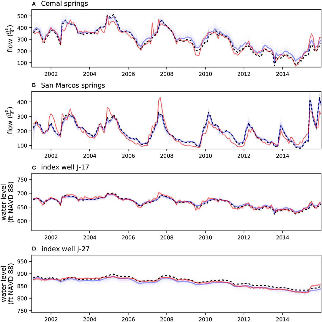
Figure 2. Observed vs. simulated plots for the four locations of primary interest to groundwater resource managers for the history-matching simulation. Red trace is the observed series, dashed black trace is the simulation results from the existing model from Liu et al. (2017), thick blue trace is the maximum a posteriori simulation result (the posterior realization corresponding to the existing model inputs), light blue traces are the posterior ensemble simulation results. In general terms, the posterior ensemble closely reproduces the observed series.

FIGURE 3

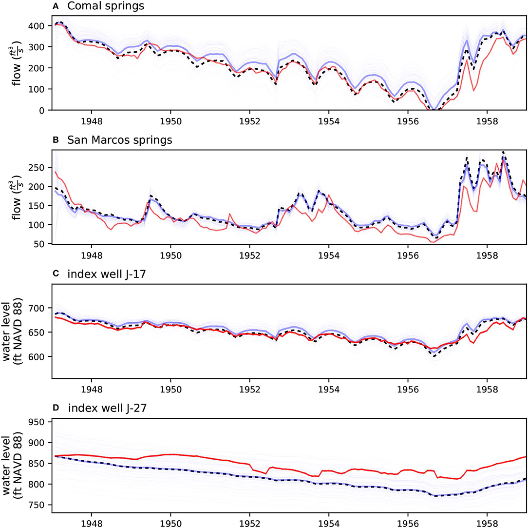
Figure 3. Observed vs. simulated plots for the four locations of primary interest to groundwater resource managers for the scenario simulation. Red trace is the observed series, dashed black trace is the existing simulation results from Liu et al. (2017), thick blue trace is the maximum a posteriori simulation result, light blue traces are the posterior ensemble simulation results. The posterior ensemble brackets the observed series, however, some uncertainty remains, which we attribute to the scenario simulation forcing parameters.

The fact that the posterior scenario simulation ensemble brackets the observed low spring-flow rates and low water levels at the springs and index wells of primary interest to groundwater resource managers (Figure 3) indicates that the combined UQ and PE analyses are likely to be robust at hindcasting (in a stochastic sense) the hydrologic response to drought at these four locations. This is an encouraging outcome and indicates that the automated workflow is functioning as expected. We attribute this success to the use of a high-dimensional parameter space (which helps to avoid under-estimation of uncertainty and limits the potential ill-effects of model error; Doherty and Christensen, 2011; White et al., 2014; Knowling et al., 2019), as well as the use of a likelihood function that was focused on outcomes of primary interest to groundwater resource managers (Doherty and Welter, 2010).

We also compared the residual ${{L}}_2$ norm (Φ) at the four locations of primary interest to groundwater resource managers for both the history-matching and scenario simulations (Figure 4). In this light, we see that the PE analysis was able to reduce Φ for both the history-matching and scenario simulation ensembles, even though the scenario simulation outputs were not used in the PE analysis. We also note that for several realizations, the posterior Φ values are less than that of the existing Liu et al. (2017) models. The reduction in Φ across the ensemble under scenario conditions is attributable to the learning through PE about the static properties in the history-matching simulation and the subsequent transfer of these static properties to the scenario simulation.

FIGURE 4

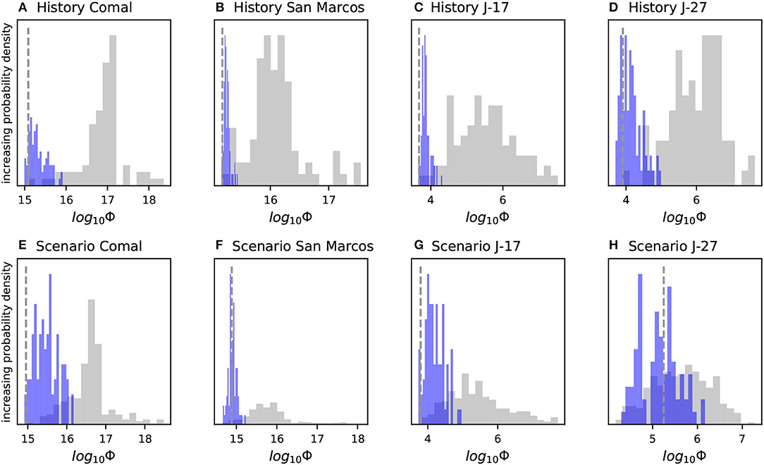
Figure 4. Prior (gray) and posterior (blue) unweighted sum of squared residual (i.e., Φ) histograms for both history-matching and scenario simulations at the four locations of primary interest to groundwater resource managers. The vertical dashed gray line marks the Φ yielded by the existing model of Liu et al. (2017). Several posterior realizations better reproduce the observed series than the existing model; the history-matching simulation ensemble is more tightly clustered around the minimum Φ.

An important aspect of PE is maintaining physically-plausible parameters (and corresponding simulation inputs). We have included several prior and posterior parameter realizations in the Supplementary Material. In general, the parameter changes resulting from the PE analysis are in agreement with the expected spatial and temporal patterns and are within the range of expectation.

The primary interest of groundwater resource managers is the number of low-flow/no-flow months at Comal springs during the scenario period. Figure 5 shows the prior and posterior statistical distribution of simulated months with flow at Comal Springs less than 30$\frac{f{t}^3}{s}$. The PE process has substantially reduced the uncertainty in this important simulated output. Specifically, the information in the state observations used for PE appears incompatible with prior realizations that yield more than 30 low-flow months. Or, put another way, parameter realizations that yield large values for Comal springs low-flow months during the scenario simulation do not fit the history-simulation observed states. Because of this incompatibility, the process of PE through history matching appears to be a valuable analysis to reduce uncertainty in the estimated Comal springs low-flow months. It is also important to note that while the posterior distributions of both of these outputs bracket their respective observed values, both consecutive months and total months of low flow contain some posterior uncertainty and could range as high as 20 and 30 months, respectively.

FIGURE 5

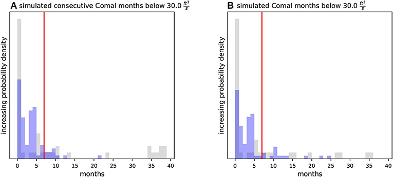
Figure 5. Prior (gray) and posterior (blue) ensemble results for (A) the consecutive months below 30 $\frac{f{t}^3}{s}$ and (B) the total months below 30 $\frac{f{t}^3}{s}$ at Comal springs during the scenario simulation. The red vertical line marks the observed values (7 months for both). The PE analyses has reduced the number of extreme cases and has moved the ensemble closer to the observed values, however, considerable uncertainty remains. Note the X-axis scale was selected to focus on the posterior realizations; 37 prior realizations yielded greater than 40 consecutive months below 30 $\frac{f{t}^3}{s}$ and 44 prior realizations yielded greater than 40 total months below 30 $\frac{f{t}^3}{s}$; these prior realizations are not shown.

5. Discussion and Conclusion

We have presented a demonstration of an approach to increase the reproducibility of UQ and PE for decision-support-scale groundwater modeling. This approach is predicated on the use of scripting to “drive” the modeling workflow. We recognize that not all environmental simulation practitioners will be proficient with scripting to the point that the approach we have demonstrated will be efficient. However, this approach offers many benefits, mostly toward increased transparency and reproducibility of the decision-support analyses—analyses that are typically at the center of the decision-making process. Furthermore, a script-based workflow affords increased efficiency when unforeseen factors arise that necessitate completing the analysis repeatedly. These “redos” are inevitable given the “ubiquity of errors” in computational science (e.g., Donoho et al., 2008) and occur, for example, when input errors are discovered or when the scope/purpose of the analysis changes). Greater reproducibility also makes the analysis more transferable to other projects and easier for third parties to evaluate or review the work (Kitzes et al., 2017).

To be clear, we are not stating that script-based analyses such as the one presented herein, will be free from input errors. While we have worked to implement the analyses herein as robustly and accurately as possible, the sheer number of operations and decisions required indicates that, in a statistical sense, there are faults or “bugs” in the script (and underlying modules) used to implement these analyses—the typical fault rate even in production-level software is between 15 and 50 faults per 1,000 lines (McConnell, 2004). However, in contrast to non-scripted modeling workflows, these “faults” can be identified and investigated by others practitioners long after the analysis has been completed—all the assumptions, decisions, and operations needed to implement our analysis are encoded transparently in the scripting workflow. This level of transparency and reproducibility has become a requirement in other fields—such as some omics cancer research—where the ramifications of decisions made in data processing can have life or death consequences (see e.g., Fienen and Bakker, 2016). Furthermore, as faults are discovered, they can be rectified programmatically in the script and the UQ and PE analyses can easily then be re-run, from beginning to end, without the complication of introducing new faults. In this way, while there is an initial “investment” to develop the scripting workflow, the returns on investment, as measured by efficiency and fidelity, are considerable.

The efficiency of the PE algorithm in PESTPP-IES has been shown to facilitate very high-dimensional (>300,000 parameters) history matching at a relatively low computational cost—the PE analysis required approximately 300 model evaluations, while the scenario prior and posterior Monte Carlo runs required approximately 100 model evaluations each. This efficiency allows practitioners to focus less on how model inputs are parameterized in the context of a computational trade-off and instead focus on expressing model input uncertainty as robustly as possible.

We realize that given the interest of groundwater resource managers in the hydrologic response to drought and the availability of state observations for PE during the scenario simulation, the scenario simulation could have also been subjected to PE (which could have easily been undertaken using our workflow and PESTPP-IES)—this would likely further reduce the posterior uncertainty in the outputs of primary interest to groundwater resource managers. However, in this study we are interested in evaluating the ability of UQ and PE to provide robust answers to management questions for which observations are not available (the more common use of environmental modeling).

Data Availability Statement

We have placed all files and codes used for the analyses presented herein in an official U.S. Geological Survey Data Release available at https://doi.org/10.5066/P9AUZMI7 (White et al., 2020). The primary workflow driver script, eaa.py, has been annotated with extensive comments to guide readers. The project repository includes pre-compiled binaries for both MODFLOW-2005 and PESTPP-IES for Linux, PC and Mac. Additionally, the repository contains the versions of the FloPy and pyEMU modules that were used. The following software versions were used:

• python 3.7.3;

• numpy (Oliphant, 2006) 1.16.4;

• pandas (McKinney, 2012) 0.25.0;

• FloPy 3.2.13;

• pyEMU 0.8; and

• PESTPP-IES 4.2.15.

Author Contributions

JWh, LF, and MF created the scripts and completed the analyses. JWh, MF, MK, and BH contributed to the development of pyEMU and FloPy that enabled the automated workflow herein and also contributed to the higher-level concepts around reproducibility through scripting. JWi provided the existing model files and also provided expert knowledge for defining the prior. JWh wrote the initial draft, however, all authors contributed to the writing of the manuscript.

Funding

The authors would like to acknowledge partial funding from the Edwards aquifer Authority under a Jointing Funding Agreement with the U.S. Geological Survey.

Disclaimers

Any use of trade, firm, or product names is for descriptive purposes only and does not imply endorsement by the U.S. Government.

This software has been approved for release by the U.S. Geological Survey (USGS). Although the software has been subjected to rigorous review, the USGS reserves the right to update the software as needed pursuant to further analysis and review. No warranty, expressed or implied, is made by the USGS or the U.S. Government as to the functionality of the software and related material nor shall the fact of release constitute any such warranty. Furthermore, the software is released on condition that neither the USGS nor the U.S. Government shall be held liable for any damages resulting from its authorized or unauthorized use.

Although these data have been processed successfully on a computer system at the U.S. Geological Survey (USGS), no warranty expressed or implied is made regarding the display or utility of the data for other purposes, nor on all computer systems, nor shall the act of distribution constitute any such warranty. The USGS or the U.S. Government shall not be held liable for improper or incorrect use of the data described and/or contained herein.

Conflict of Interest

MK and BH were employed by the GNS Science, a commercial entity owned by the New Zealand government.

The remaining authors declare that the research was conducted in the absence of any commercial or financial relationships that could be construed as a potential conflict of interest.

Acknowledgments

The authors would like acknowledge all of the contributors and maintainers of FloPy, pyEMU, and PEST++. We would also like to acknowledge Nathan Pasley for making Figure 1.

Supplementary Material

The Supplementary Material for this article can be found online at: https://www.frontiersin.org/articles/10.3389/feart.2020.00050/full#supplementary-material

The Supplementary Material included in this work includes:

• Parameter prior variance summary by group;

• Array-based multiplier parameterization summary for the first few realizations in the parameter ensemble for the active model area shown in figure 1 in main text.

References

Anderson, M. P., Woessner, W. W., and Hunt, R. J. (2015). Applied Groundwater Modeling, 2nd Edn. San Diego, CA: Academic Press.

Bakker, M., Post, V., Langevin, C. D., Hughes, J. D., White, J. T., Starn, J. J., et al. (2016). Scripting modflow model development using python and flopy. Groundwater 54, 733–739. doi: 10.1111/gwat.12413

PubMed Abstract | CrossRef Full Text | Google Scholar

Barchard, K., and Pace, L. (2011). Preventing human error: the impact of data entry methods on data accuracy and statistical results. Comput. Hum. Behav. 27, 1834–1839. doi: 10.1016/j.chb.2011.04.004

CrossRef Full Text | Google Scholar

Beven, K., and Binley, A. (1992). The future of distributed models: model calibration and uncertainty prediction. Hydrol. Process. 6, 279–298. doi: 10.1002/hyp.3360060305

CrossRef Full Text | Google Scholar

Brakefield, L. K., White, J. T., Houston, N. A., and Thomas, J. V. (2015). Updated Numerical Model With Uncertainty Assessment of 1950-56 Drought Conditions on Brackish-Water Movement Within the Edwards Aquifer, San Antonio, Texas. U.S. Geological Survey Scientific Investigations Report 2015–5081. doi: 10.3133/sir20155081

CrossRef Full Text | Google Scholar

Chen, Y., and Oliver, D. S. (2013). Levenberg–marquardt forms of the iterative ensemble smoother for efficient history matching and uncertainty quantification. Comput. Geosci. 17, 689–703. doi: 10.1007/s10596-013-9351-5

CrossRef Full Text | Google Scholar

Chen, Y., and Oliver, D. S. (2016). Localization and regularization for iterative ensemble smoothers. Comput. Geosci. 21, 1–18. doi: 10.1007/s10596-016-9599-7

CrossRef Full Text | Google Scholar

Doherty, J. (2003). Ground water model calibration using pilot points and regularization. Ground Water 41, 170–177. doi: 10.1111/j.1745-6584.2003.tb02580.x

PubMed Abstract | CrossRef Full Text | Google Scholar

Doherty, J. (2015a). Calibration and Uncertainty Analysis for Complex Environmental Models - PEST: Complete Theory and What It Means for Modeling the Real World. (Brisbane, QLD: Watermark Numerical Computing).

Doherty, J., and Christensen, S. (2011). Use of paired simple and complex models to reduce predictive bias and quantify uncertainty. Water Resour. Res. 47. doi: 10.1029/2011WR010763

CrossRef Full Text | Google Scholar

Doherty, J., and Welter, D. (2010). A short exploration of structural noise. Water Resour. Res. 46. doi: 10.1029/2009WR008377

CrossRef Full Text | Google Scholar

Doherty, J. E. (2015b). PEST and Its Utility Support Software, Theory. (Brisbane, QLD: Watermark Numerical Publishing).

Doherty, J. E., Hunt, R. J., and Tonkin, M. J. (2011). Approaches to Highly Parameterized Inversion: A Guide to Using PEST for Model-Parameter and Predictive-Uncertainty Analysis. Geological Survey Scientific Investigations Report 2010-5211.

Google Scholar

Donoho, D. L., Maleki, A., Rahman, I. U., Shahram, M., and Stodden, V. (2008). Reproducible research in computational harmonic analysis. Comput. Sci. Eng. 11, 8–18. doi: 10.1109/MCSE.2009.15

CrossRef Full Text | Google Scholar

Fienen, M. N., and Bakker, M. (2016). Hess opinions: Repeatable research: what hydrologists can learn from the duke cancer research scandal. Hydrol. Earth Syst. Sci. 20, 3739–3743. doi: 10.5194/hess-20-3739-2016

CrossRef Full Text | Google Scholar

Fienen, M. N., and Hunt, R. J. (2015). High-throughput computing versus high-performance computing for groundwater applications. Groundwater 53, 180–184. doi: 10.1111/gwat.12320

PubMed Abstract | CrossRef Full Text | Google Scholar

Fisher, J. C. (2014). “wrv: an R package for groundwater flow model construction, Wood River Valley Aquifer System, Idaho,” in AGU Fall Meeting Abstracts (San Francisco, CA).

Google Scholar

Fisher, J. C., Bartolino, J. R., Wylie, A. H., Sukow, J., and McVay, M. (2016). Groundwater-Flow Model for the Wood River Valley Aquifer System, South-Central Idaho. in U.S. Geological Survey Scientific Investigations Report 2016-5080 (Reston, VA), 84. doi: 10.3133/sir20165080

CrossRef Full Text | Google Scholar

Goecks, J., Nekrutenko, A., and Taylor, J. (2010). Galaxy: a comprehensive approach for supporting accessible, reproducible, and transparent computational research in the life sciences. Genome Biol. 11:R86. doi: 10.1186/gb-2010-11-8-r86

PubMed Abstract | CrossRef Full Text | Google Scholar

Hanke, M. (1997). A regularizing levenberg-marquardt scheme, with applications to inverse groundwater filtration problems. Inverse Prob. 13:79. doi: 10.1088/0266-5611/13/1/007

CrossRef Full Text | Google Scholar

Harbaugh, A. W. (2005). MODFLOW-2005, the U.S. Geological Survey modular ground-water model – the Ground-Water Flow Process (Reston, VA), Vol. 6. doi: 10.3133/tm6A16

CrossRef Full Text | Google Scholar

Kitzes, J., Turek, D., and Deniz, F. (2017). The Practice of Reproducible Research: Case Studies and Lessons From the Data-Intensive Sciences. (Berkeley, CA: Univ of California Press).

Google Scholar

Knowling, M. J., White, J. T., and Moore, C. R. (2019). Role of model parameterization in risk-based decision support: an empirical exploration. Adv. Water Resour. 128, 59–73. doi: 10.1016/j.advwatres.2019.04.010

CrossRef Full Text | Google Scholar

Lindgren, R. J., Dutton, A. R., Hovorka, S. D., Worthington, S. R., and Painter, S. (2005). “Conceptualization and simulation of the Edwards aquifer, San Antonio region, Texas,” in Sinkholes and the Engineering and Environmental Impacts of Karst (Reston, VA), 122–130. doi: 10.1061/40796(177)14

CrossRef Full Text | Google Scholar

Liu, A., Troshanov, N., Winterle, J., Zhang, A., and Eason, S. (2017). Updates to the Modflow Groundwater Model of the San Antonio Segment of the Edwards Aquifer. in Edwards Aquifer Authority Technical Report (San Antonio, TX).

Google Scholar

Liu, Z., Wang, S. P., and Meyer, D. (2019). Improving reproducibility in earth science research. EOS 100. doi: 10.1029/2019EO136216

CrossRef Full Text

McConnell, S. (2004). Code Complete. (Sebastopol, CA: Pearson Education).

McKenna, S. A., Akhriev, A., Ciaurri, D. E., and Zhuk, S. (2019). Efficient uncertainty quantification of reservoir properties for parameter estimation and production forecasting. Math. Geosci. 233–251. doi: 10.1007/s11004-019-09810-y

CrossRef Full Text | Google Scholar

McKinney, W. (2012). Python for Data Analysis: Data Wrangling with Pandas, NumPy, and IPython. O'Reilly Media.

Google Scholar

Moore, C., and Doherty, J. E. (2005). Role of the calibration process in reducing model predictive error. Water Resour. Res. 41, 1–14. doi: 10.1029/2004WR003501

CrossRef Full Text | Google Scholar

Oliphant, T. E. (2006). Guide to NumPy. Provo, UT.

PubMed Abstract | Google Scholar

Olsthoorn, T. (2010). “Improved groundwater modeling using an open and free environment called Mflab,” in NGWA 2010 Groundwater Summit (Denver, CO).

Peng, R. D. (2011). Reproducible research in computational science. Science 334, 1226–1227. doi: 10.1126/science.1213847

PubMed Abstract | CrossRef Full Text | Google Scholar

Plesser, H. E. (2018). Reproducibility vs. replicability: a brief history of a confused terminology. Front. Neuroinformat. 11:76. doi: 10.3389/fninf.2017.00076

PubMed Abstract | CrossRef Full Text | Google Scholar

Puente, C. (1978). Method of estimating natural recharge to the edwards aquifer in the san antonio area, texas. Sci. Investigat Rep. doi: 10.3133/wri7810. [Epub ahead of print].

CrossRef Full Text | Google Scholar

Sandve, G. K., Nekrutenko, A., Taylor, J., and Hovig, E. (2013). Ten simple rules for reproducible computational research. Pub. Lib. Sci. Comput. Biol. 9. doi: 10.1371/journal.pcbi.1003285

PubMed Abstract | CrossRef Full Text | Google Scholar

Stodden, V. (2010). “The scientific method in practice: reproducibility in the computational sciences,” in MIT Sloan Research Paper No. 4773-10. 33. doi: 10.2139/ssrn.1550193

CrossRef Full Text | Google Scholar

Tarantola, A. (2005). Inverse Problem Theory and Methods for Model Parameter Estimation. (Philadelphia, PA: SIAM). doi: 10.1137/1.9780898717921

CrossRef Full Text | Google Scholar

Thain, D., Tannenbaum, T., and Livny, M. (2005). Distributed computing in practice: the condor experience. Concur. Pract. Exp. 17, 323–356. doi: 10.1002/cpe.938

CrossRef Full Text | Google Scholar

White, J. T. (2018). A model-independent iterative ensemble smoother for efficient history-matching and uncertainty quantification in very high dimensions. Environ. Model. Softw. 109, 191–201. doi: 10.1016/j.envsoft.2018.06.009

CrossRef Full Text | Google Scholar

White, J. T., Doherty, J. E., and Hughes, J. D. (2014). Quantifying the predictive consequences of model error with linear subspace analysis. Water Resour. Res. 50, 1152–1173. doi: 10.1002/2013WR014767

CrossRef Full Text | Google Scholar

White, J. T., Fienen, M. N., and Doherty, J. E. (2016). A python framework for environmental model uncertainty analysis. Environ. Model. Softw. 85, 217–228. doi: 10.1016/j.envsoft.2016.08.017

CrossRef Full Text | Google Scholar

White, J. T., Foster, L. K., Fienen, M. N., Knowling, M. J., Hemmings, B., and Winterle, J. R. (2020). Data release for “towards reproducible environmental modeling for decision support: a worked example,” (Reston, VA: U.S.Geological Survey Data Release).