Characteristics of Slow Slip Event in March 2020 Revealed From Borehole and DONET Observatories

Introduction

In the wake of the 2004 Sumatra-Andaman earthquake (e.g., Wiseman and Bürgmann, 2011), the Japanese government has established seafloor networks of cable-linked observatories around Nankai Trough (Figure 1): DONET (Dense Oceanfloor Network system for Earthquakes and Tsunamis along the Nankai Trough) which has sensors of broadband seismogram, strong ground motion, and hydraulic pressure (e.g., Kaneda et al., 2015; Kawaguchi et al., 2015). DONET has been expected to monitor the propagation process of tsunami (e.g., Maeda et al., 2015) and seismic waves (Nakamura et al., 2015) as well as seismic activity (Nakano et al., 2016; 2018) in real time.

FIGURE 1

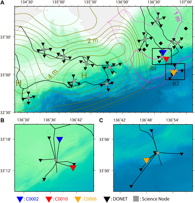
FIGURE 1. A) Map of the borehole observatories and DONET stations along Nankai Trough. The triangle marks (▼ blue, ▼ red, ▼ yellow, and ▼ black) represent C0002, C0010, and C0006 of the borehole observatories and the DONET stations, respectively. The diamonds represent the GNSS-A stations. The magenta and olive contours represent the slip distributions of the 1944 Tonankai and 1946 Nankai earthquakes, respectively (Ichinose et al., 2003; Murotani et al., 2015). Their contour interval is 0.5 m. L and H: regions of low and high slip, respectively. (B) Closeup of C0002 and C0010 of the borehole observatories and D-node of the DONET station. (C) Closeup of C0006 and C-node.

Owing to inland dense networks of seismic and geodetic observations have revealed that slow earthquakes occur along the subduction plate boundaries in the shallower and deeper extensions of megathrust earthquake source regions worldwide (e.g., Schwartz and Rokosky, 2007; Obara and Kato, 2016). Slow earthquake is assumed to be classified into several types according to the spatiotemporal scale (Ide et al., 2007). For example, low-frequency tremor and very low-frequency events (VLFEs) have dominant periods of approximately several hertz (Obara, 2002) and 10–100s (Ito et al., 2007), respectively, whereas slow slip events (SSEs) have a duration time of days to years (Dragert et al., 2001).

As a Japanese governmental organization, Earthquake Research Committee of the Headquarters for Earthquake Research Promotion (2013) has pointed out the possibility of megathrust earthquakes occurring along Nankai in the near future. Slow earthquake is more sensitive to stress change than a regular earthquake (Obara and Kato, 2016); hence, it is important to monitor slow earthquake activities close to a megathrust earthquake. Some numerical simulations have demonstrated that the recurrence interval and the moment release rate of VLFEs/SSEs become shorter and higher, respectively, in the pre-seismic stage of a megathrust earthquake (Matsuzawa et al., 2010; Ariyoshi et al., 2012).

For the shallower slow earthquakes occurred in the shallower extension, these changes are expected to be larger than those in the deeper one from numerical simulation study (Ariyoshi et al., 2014a; Ariyoshi et al., 2014b). Shallower VLFEs near the trench (sVLFE) has been detected around the Nankai Trough not only by seafloor cabled networks (Nakano et al., 2016; Nakano et al., 2018; Nishikawa et al., 2019) but also by inland seismic networks (Takemura et al., 2019). By contrast, the shallower SSE near the trench has so far been detected only from the pore pressure change of the borehole observatories (Wallace et al., 2016; Araki et al., 2017) and the seafloor global navigation satellite system-acoustic (GNSS-A) (Ishikawa et al., 2020) because the SSE can be detected by static crustal deformation with distance r⁻³ decay, which is too small for inland GNSS networks. However, the data of the borehole observatories at that time were offline. GNSS-A is also offline, and its time resolution of the SSE signal detection is 0.2 years (Yokota and Ishikawa, 2020).

Recently, the borehole observatories in holes C0002 (Figure 2), C0010, and C0006 were successfully connected to DONET: C0002 in January 2013 (Kitada et al., 2013), C0010 in April 2016 (Saffer et al., 2017), and C0006 in March 2018. This operation has enabled us to monitor crustal deformation along the Nankai Trough in real time. Afterward, in the latter part of March 2020 (Figure 3), significant change of pore pressure (we refer to “pore pressure event”) and five sVLFEs were detected by the borehole site C0002 and broadband seismometers of DONET, respectively. On the other hand, there is no signal at C0006. For C0010, there appears pore pressure change during that time, but it seems not to be stable before and after that period. This instability began after the replacement operation of the sensors, which means the possibility that the record of the pore pressure at C0010 contains both crustal deformation and other unrecognized fluctuations. Therefore, it is very important to examine whether those changes could be explained by a reasonable fault model of SSE or not. In the present study, we first reviewed the pore pressure change and sVLFE activity. Next, we investigate the time history of pore pressure change at C0002 by fitting regression lines. Using these results, we try to find reasonable fault models for the pore pressure event by considering possible cases of pore pressure change at C0010, the observed sVLFE, and the characteristics of previous SSEs when C0010 was stable. To evaluate the reliability of pore pressure record at C0010, we conduct t-test between the pore pressure event and the unrecognized fluctuation for yearlong data before the pore pressure event. Finally, we discussed the detectability of the seafloor crustal deformation caused by the possible fault models, toward monitoring the plate coupling around the Nankai Trough.

FIGURE 2

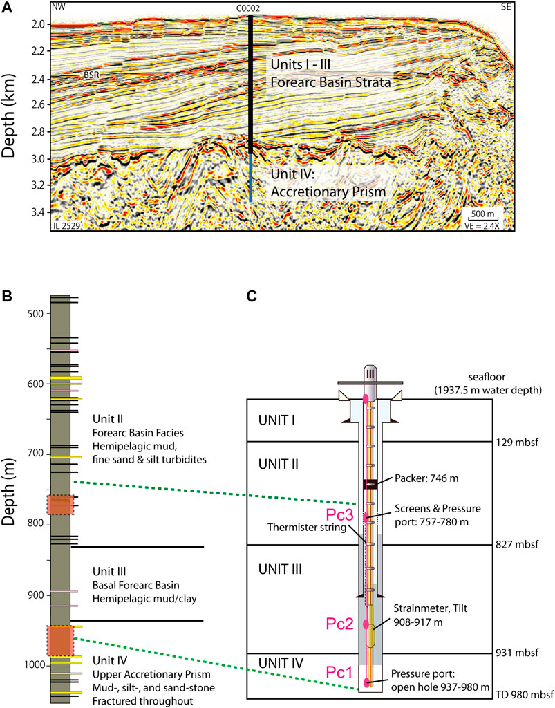
FIGURE 2. (A) Seismic section showing the location of the borehole observatory installation at C0002. (B) Schematic stratigraphic column. Gray: clay and mudstone. Black: silt. Yellow: sand. Pink: ash. (C) Borehole completion diagram. The solid magenta ellipses indicate the pressure gauges, where the top one is a hydrostatic reference pressure sensor used to remove oceanographic signals. This figure is modified after the Supplemental Material of Araki et al. (2017).

FIGURE 3

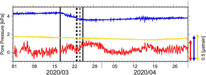
FIGURE 3. Time history of the pore pressure at the deepest stations (Pc1) of each borehole observatory with a volumetric scale for each station (vertical double arrows). The oceanic signals are reduced by the reference hydraulic pressure gauge on the seafloor. The bold lines represent the onset/termination time of the pore pressure event. The dotted lines represent the origin times of the sVLFEs (Table 1).

Pore Pressure Change at Boreholes

Three borehole observatories (i.e., C0002, C0010, and C0006) in the sedimentary wedge can be found above the subduction plate boundary in the Nankai Trough. An overview of the observatory station at C0002, which is the main target of the present study, is shown in Figure 2. We have continuously monitored the crustal deformations, using the pore pressure changes observed by the sensors installed in finely grained sediments with low permeability. For each observatory, two or three sensors were installed at hydraulically isolated depth intervals (C0002: 1966 m depth below sea level [mbsl], Pc1: 937–980 m depth below seafloor [mbsf], and Pc2: 908–917 mbsf, Pc3: 757–780 mbsf; C0010: 2524 mbsl, Pc1: 610 mbsf, and Pc3: 405 mbsf; C0006: 3872 mbsl, Pc1: 456 mbsf, and Pc2: 426 mbsf). We focused herein on the deepest pore pressure (Pc1) at each borehole to see the crustal deformation close to the subduction plate boundary.

The pore pressure change mainly reflects the contributions from the following components: volumetric strain change driven by the crustal deformation in the accretionary prism several kilometers above the plate interface (Davis et al., 2006), ocean tides and other oceanographic loading (Araki et al., 2017), and dynamic deformation due to the passage of seismic waves radiated from earthquakes (Katakami et al., 2020). We removed the oceanic loading using the reference pressure sensor on the seafloor co-located for each observatory (Araki et al., 2017). The value of coefficient (α) for the reference pressure is obtained by the method of least squares for R=(Pc1–α*Pc0).

If the pore pressure change is derived from elastic deformation, we can linearly convert it to the volumetric strain change. From previous studies, the conversion factors are obtained for each Pc1 at C0002 (5.7 kPa/μstrain), C0010 (4.7 kPa/μstrain), and C0006 (6.0 kPa/μstrain) (Davis et al., 2006; Wallace et al., 2016; Araki et al., 2017). Therefore, monitoring of the pore pressure change is useful to evaluate the crustal deformation.

Figure 3 shows the time history of Pc1 at each borehole from March to April in 2020 with the oceanic signals reduced, which suggests that pore pressure change at C0002 is similar to ramp function. This feature could not be explained from the oceanic loading. If this change is due to crustal deformation, the volumetric strain at C0002 had a significant dilation change (estimated as −0.14 μstrain) on March 17–26, 2020. By contrast, no significant change was observed at C0006. As mentioned in the introduction section, C0010 has already the unrecognized fluctuation before the pore pressure event. This means that we have to extract the crustal deformation component if the pore pressure event is driven by SSE, which is to be discussed in the following sections.

sVLFE Activities Beneath the Borehole Observatories

Figure 4A shows past sVLFE activities off Tonankai and Nankai regions, which indicates that sVLFE is active locally around the strong coupling regions of the megathrust earthquakes. In the target area, sVLFE had occurred in the marginal part of the 1944 Tokai earthquake and the transition zone to the 1946 Nankai earthquake. From the previous results, the previous SSE source areas coincided with the sVLFE locations (Sugioka et al., 2012; Obara and Kato, 2016), and the sVLFEs were temporally excited during the SSE (Araki et al., 2017; Nakano et al., 2018).

FIGURE 4

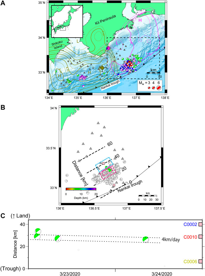
FIGURE 4. (A) Past seismic activities in the study area. The gray triangles represent the locations of the DONET stations. The epicentral distribution of the focal mechanism for the sVLFE occurred in 2003–2004 (green: Obara and Ito, 2005; Ito and Obara 2006), 2009 (red: Sugioka et al., 2012), 2015 (purple: Nakano et al., 2016), and 2016 (blue: Nakano et al., 2018). Epicenters of the 1944 Tonankai and 1946 Nankai earthquakes are represented by magenta and olive diamonds, respectively. The magenta and olive contours are the same as Figure 1A. (B) Closeup of the rectangle region enclosed by black broken lines in (A). The gray and green focal mechanisms represent the sVLFE catalog in 2016 (Nakano et al., 2018) and the latest one accompanied by the pore pressure event, respectively. The pink squares represent the borehole stations buried with the focal mechanism in (A). The dotted rectangles represent the fault models of Case A-1 (cyan) and Case A-2 (magenta) (A-2 is smaller, A-2+ is larger) for the pore pressure event (Figure 6). (C) Activities of the sVLFEs in March 2020 along the dip direction from the Nankai Trough with the same color scale of the depth profile in (B). The dotted lines depict the migration speed at 4 km/day estimated by Nakano et al. (2018), where the interval of the two dotted lines is 5 km as a spatial resolution for the epicenter determination.

We found the five sVLFEs between March 23 and 24, 2020 from the broadband velocity seismograms of the DONET stations along Nankai Trough. The sVLFE catalog during that period, indicating that one of them is a doublet event spatiotemporally, is shown in Table 1. We applied a centroid moment tensor waveform inversion to the broadband velocity seismometers at each DONET station (Nakano et al., 2018) during the pore pressure event to determine the source location, fault orientation parameters, and moment magnitude of the sVLFEs. The obtained source location and moment magnitudes are listed in Table 1, where horizontal and vertical resolution is 5 and 2 km, respectively.

TABLE 1

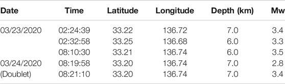
TABLE 1. sVLFE catalog in March 2020.

Figure 4B shows the focal mechanisms of the sVLFEs were low-angle thrust-type faults largely along the plate interface. These results are consistent with previous sVLFE activities (Figure 4A). The hypocenter distribution of the sVLFEs in 2020 overlapped the source regions of past sVLFEs in part of the large slip area of the great 1944 Tonankai earthquake (Ichinose et al., 2003).

The time history of the sVLFEs along the horizontal distance from the trench is shown in Figure 4C. As suggested in Figures 4B,C, the spatiotemporal change of the five sVLFEs in 2020 appeared to be characterized by a migration from downdip to updip toward the trench (Figure 4C). This result is similar to the previous SSE in 2016, whose migration rate was approximately 4 km/day (Nakano et al., 2018).

These results imply that the pore pressure event is driven by SSE migrating toward the trench and the time history of pore pressure at C0010 may partly have crustal deformation component, which is discussed in the following sections.

Estimation of the Onset/Termination Time and the Pore Pressure Change at C0002

The duration time of the SSE was estimated in days (Araki et al., 2017; Table 2), whereas the origin time of the sVLFE was estimated in seconds (or less). This might cause difficulty to investigate the relationship between the SSE and sVLFE. One of the reasons of the daily solution for the SSE duration time is that the change in rate of the pore pressure at the beginning and ending of SSEs appears insufficiently clear, which is difficult to estimate the duration time precisely. We compensated for the gap of the time precision by trying to quantitatively estimate the amount of the pore pressure change and the onset/termination time of the pore pressure event in March 2020 by fitting regression lines, focusing on C0002 because of its simple behavior.

TABLE 2

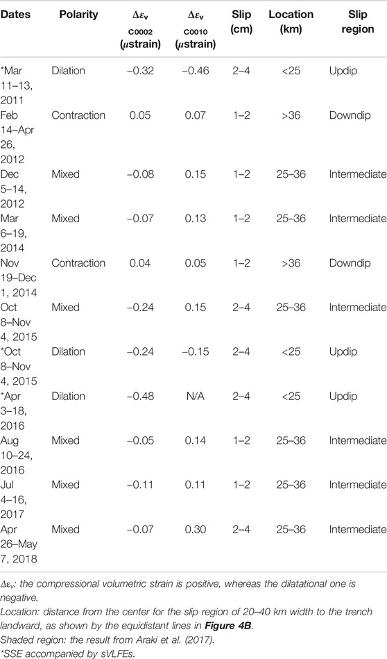
TABLE 2. Updated summary of the borehole pressure signals and SSE characteristic.

The time history of the pore pressure change at C0002 could be separated into three periods as before, during, and after the pore pressure event (Figure 3). Before and after the pore pressure event, linear regression analysis is well applicable with trend negligible. During the pore pressure event, however, a temporal decrease of the pore pressure was observed (hidden in Figure 3 because of decimation operation), which could not be explained by the regression analysis and will be discussed later.

To avoid a wrong regression estimation caused by such an unrecognized perturbation during the pore pressure event, we only estimated the two regression lines before and after the pore pressure event by treating the onset and the termination time of the pore pressure event as unknown parameters. The remaining regression line during the pore pressure event can be obtained by connecting both edges of the two regression lines before and after the pore pressure event, which gives the change amount of the pore pressure during the event. We select the input data span from March 1 to April 9, 2020 so that the periods of before, during and after the pore pressure event is comparable, where this choice of the date range is not critical for the following result. We adopted the least absolute value (L1 norm) to the evaluation function for all input data of 20 min sampling, moving the onset and the termination time during the data period at a 20 min interval. Although we also investigated other methods, such as the least squares method (L2 norm) with the time sampling changed, these methods could not obtain reasonable solutions.

Table 3 shows the results of best solution for each sensor at C0002. The standard deviations of the onset/termination time and the pore pressure change are 1.0 days and 1.0 hPa (1.1 days and 1.7 hPa for Pc3), respectively. Without the temporal decrease, the standard deviations are 9 h and 0.4 hPa, respectively. The time history of the pore pressure change compared with the regression lines of the analytical solution is shown in Figure 5. Since the time lag from the origin time of sVLFEs to the termination time of the pore pressure event (1 day and 20 min) is larger than the standard deviation (0.375 or 1.0 days), we statistically conclude that the sVLFE occurred during the pore pressure event.

TABLE 3

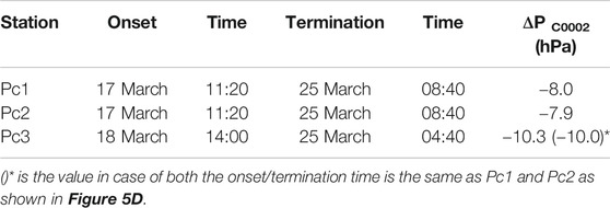
TABLE 3. Estimation results of pore pressure change due to the SSE in 2020.

FIGURE 5

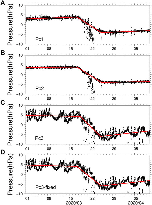
FIGURE 5. Time history of the pore pressure (dotted black: 20 min sampling) with the fitting regression lines (red) for (A) Pc1, (B) Pc2, (C) Pc3, and (D) Pc3 under the same time of onset and termination as Pc1 and Pc2.

From Table 3 and Figures 5A–C, the best solution of Pc3 has shorter duration time due to the later onset and the earlier termination times than Pc1/Pc2. Figure 5C also shows that ocean noise component for Pc3 is significantly larger than that for Pc1 and Pc2. This means that the determination of the onset/termination time of the pore pressure event for Pc3 may not be robust. Figure 5D shows another regression combination for Pc3, assuming the onset/termination time is the same as Pc1 and Pc2, which seems also consistent with observation data. The amounts of pore pressure changes for Pc3 in Figures 5C,D are −10.3 and −10.0 hPa, respectively. This result suggests that the amplitude of ΔP for Pc3 is larger than Pc1 and Pc2, which is consistent with static dislocation model (Okada, 1992) due to the free surface condition.

Possibility of SSE for the Pore Pressure Event

In Figure 3, the unrecognized fluctuation of pore pressure at C0010 seems to be classified into (about daily) periodic and systematic components of non-crustal deformation. The amplitude of the systematic component is sometimes greater than that of periodic one. This means that it is not reasonable to estimate the onset/termination time and the amount of pore pressure change at C0010 solely from the time history. To evaluate the amount of pore pressure change statistically, we have to classify the time history of pore pressure change at C0010 into the signal (crustal deformation component), the systematic error and periodic perturbation.

In this section, we try to find a reasonable time series of pore pressure change at C0010 and discuss the validity of identifying the pore pressure event as SSE by considering our results mentioned above and characteristics of previous SSEs.

Possible Cases of the Onset/Termination Times and Volumetric Strain Change at C0010

First, we compare the pore pressure event with previous SSEs which accompanied sVLFE. From Table 2, the corresponding SSEs occurred in 2011, 2015 and 2016. Unfortunately, the pore pressure record at C0010 was not obtained for SSE in 2016. Hence, we focus on the SSEs in 2011 and 2015. Since these SSEs occurred before the replacement of sensors at C0010, the quality of pore pressure record at C0010 was as good as C0002. For these SSEs, the onset and termination time of the pore pressure change is almost simultaneous between C0002 and C0010 (Araki et al., 2017). Therefore, we focus on the pore pressure records of the pore pressure event between the onset and termination times estimated in the preceding section (17 March 11:20 to 25 March 08:40; as listed in Table 3) as shown in Figures 5A,B.

On the basis of the time history of pore pressure at C0010 during the event, we assume four possible cases as shown by arrows in Figure 6. Case A is derived from the SSE in 2015, which is divided into the increase (A-1) and decrease (A-2) cases of the pore pressure. This means that the crustal deformation of SSE is composed of Cases A-1 and A-2, where the latter part of increase at C0010 in Figure 6 is treated as unrecognized noise component. In addition, we also assume Case A-2+, whose dilation lasts for the dilation of C0002 time as shown by dotted line in Figure 6, in according to SSE in 2015 (Araki et al., 2017). Case B assumes that the latter part of increase is the crustal deformation component. Case C assumes that the decrease of pore pressure is the unrecognized noise and the crustal deformation is described as monotonic increase. Case D assumes that there is no signal like C0006.

FIGURE 6

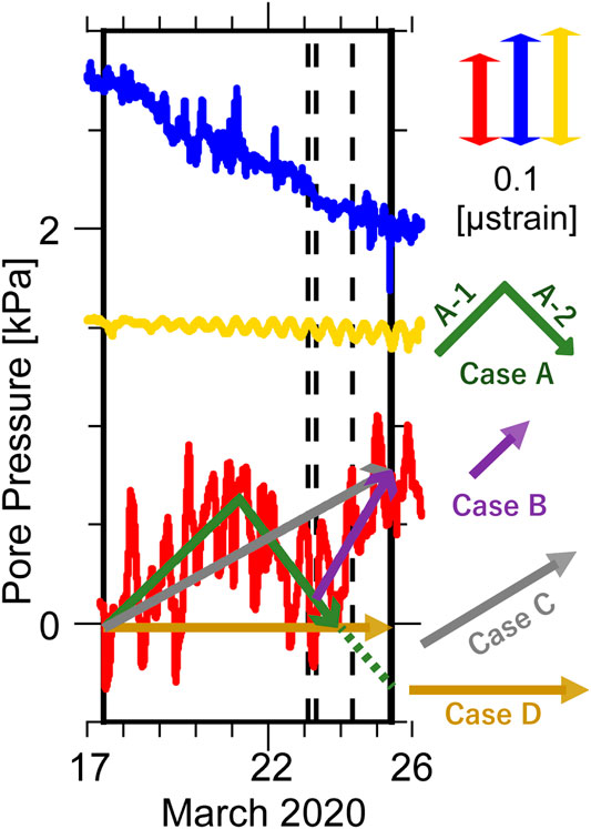
FIGURE 6. Close up of the time history of the pore pressure (Figure 3) during the event, where the onset/termination time is determined by Figures 5A,B. Arrows indicate possible cases for the time histories of crustal deformation component at C0010 determined by regression lines (see text). The dotted lines represent additional Cases A-2+ and C+ as listed in Table 4.

To estimate the pore pressure change at C0010 for each Case and onset times for Cases A-2 and Case B, we apply the same regression analysis as Figure 5 to C0002 by treating the error of periodic component of fluctuation approximately as a Gaussian distribution. Figure 6 shows the best solutions of regression lines for each Case. The amounts of volumetric strain changes at C0002 and C0010 for each Case and the onset times for Case A-2 and Case B are listed in Table 4, where the volumetric strain changes at C0002 for Cases A-1, A-2 and B are determined by the onset/termination times under the constant decrease rate of the best regression analysis in Figure 5. The standard deviations of the pore pressure change at C0010 and onset time are 2.1 hPa (∼0.045 μstrain) and 0.86 days, respectively.

TABLE 4

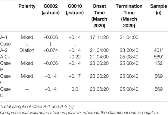
TABLE 4. Possible cases of the volumetric strain change due to the SSE in 2020.

Statistical Evaluation of Confidence for Each Case of Pore Pressure Change at C0010

As mentioned in Section Possible Cases of the Onset/Termination Times and Volumetric Strain Change at C0010, we assume that the pore pressure change at C0010 contains crustal deformation component between the onset and termination times estimated from C0002. However, there is still possibility that the pore pressure change at C0010 during that time span is due to unrecognized fluctuation. In this section, we try to evaluate the statistical confidence of the crustal deformation component at C0010 for each Case in Figure 6.

To verify the possibility of crustal deformation at C0010 due to SSE statistically, we adopt the minimum square method for the regression lines of all Cases in Figure 6,

$S\left(i\right)={\left\{y\left(t_i\right)-f_{\left(\text{A,B,C,D}\right)}\left(t_i\right)\right\}}^2,(1)$

$U=\left\{S_1,S_2,\dots ,S_n\right\},(2)$

where t and i are time and its index, respectively. y and f_(A,B,C,D) are observational data and the regression analysis in Figure 6, respectively. n is the number of 20 min sampling for each Case as listed in Table 4. For the pore pressure event (Figure 6), the average and standard deviation of S(i) in U_(A,B,C,D) are obtained as $\overline{S}$ and σ.

Since the last SSE occurred in May 2018 (Table 2), we can treat the yearlong data from 16 March in 2019 to 16 March in 2020 (Figure 7) as the reference of the unrecognized fluctuation. If the time series of pore pressure change at C0010 in Figure 6 were due to the unrecognized fluctuation, similar change would occur in the yearlong period. For the yearlong data, we calculate ${\overline{S}}^{\prime }$ and ${\sigma }^{\prime }$ with the same number of sampling as the regression lines for each Case (Table 4), moving the time window by one sampling at a time from the beginning to the end of the yearlong data.

FIGURE 7

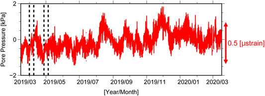
FIGURE 7. Time history of the pore pressure at the deepest stations (Pc1) of C0010 with a volumetric scale for each station (vertical double arrows) from one year before to the one day before the onset time of the pore pressure event. Two pairs of vertical dotted lines indicate the time windows of best fitting regression lines for Case (A-1) to (A-2+) as indicated by vertical arrows in Figure 8.

If the pore pressure change at C0010 in Figure 6 is significantly different from the unrecognized fluctuation (Figure 7), there should be always significant difference between $\overline{S}$ and ${\overline{S}}^{\prime }$ for all the time window in the yearlong period. Here, we apply two-sample t-test between ($\overline{S}$, $\sigma$) and (${\overline{S}}^{\prime }$, ${\sigma }^{\prime }$) for each moving time window to verify whether $\overline{S}<{\overline{S}}^{\prime }$ or not, where the value of t statistics is described as

$t=\frac{S^{\prime }-S}{\sqrt{\left({\sigma }^2+{\left({\sigma }^{\prime }\right)}^2\right)/n}},(3)$

and t distribution is approximated as the standard normal distribution function because of high degree of freedom (n−1 >100).

Figure 8 shows the time history of t statistics for each Case. Figures 8A,B show that the value of t statistics is basically positive (>5). For Case (A-1) to (A-2+), the (negative) minimum value of the t statistics is -0.84 for the time window between 27 April 08:40 and 5 May 05:40 in 2019 and -0.74 between 31 March 20:00 and 8 April 16:40 (dotted lines in Figure 7). These mean that the probability of $\overline{S}<{\overline{S}}^{\prime }$ is 20% and 27%, respectively. For the other Cases, Figure 8 shows that there are many time windows with the t statistics less than -5, where the probability of $\overline{S}<{\overline{S}}^{\prime }$ is less than 0.01%. From these results, Cases B, C, and D could not be distinguished from the unrecognized fluctuation, and the reliability of Case (A-1) to (A-2+) for crustal deformation component is at most 20% because of low S/N ratio. In the following sections, we try to enhance the reliability of pore pressure change at C0010 by considering sVLFE activities as well as pore pressure changes at other borehole sites.

FIGURE 8

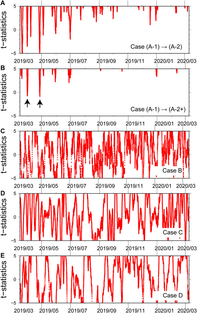
FIGURE 8. Time history of t-statistics in Eq. (3) for each Case. Horizontal axis is origin time of fitting time window. Positive value of t-statistics means regression lines explain crustal deformation component due to SSE better than unrecognized fluctuation. Vertical arrows indicate the minimum value of t-statistics for Case (A-1) to (A-2+), where corresponding time windows are indicated by two pairs of vertical dotted lines in Figure 7.

Relationship Between the Volumetric Strain Change and Fault Location of SSE

Because of the insufficient number of borehole observatories, it is practically difficult to estimate the fault parameters by inversion method. In this study, we assume that SSE occurred on the plate interface beneath the borehole observatories, according to the previous method (Wallace et al., 2016; Araki et al., 2017).

We set up the fault location, fault width, and fault displacement as unknown parameters which well explain the two volumetric strain changes at C0002 and C0010. Considering the spatial resolution due to limited observations, we assume that the epicentral location for the center point of fault is along the line between C0002 and C0010, the width is 20 or 40 km, and the displacement is 1-2 or 2–4 cm. The forward modeling assumed a simple rectangular fault model (Okada, 1992) in a homogeneous elastic medium with a Poisson’s ratio of 0.35 and a rigidity of 20 GPa, which is the same condition as Araki et al. (2017). The simplified fault model assumed that the direction angles of strike, dip, and rake were 239° (along subduction direction), 6°, and 90°, respectively, where the strike direction was orthogonal to the equidistant lines from the trench in Figure 4B.

For the previous SSEs, the polarities of the volumetric strain changes at C0002 and C0010 reflects the relative location between the two sites and SSE (Araki et al., 2017). Following the result, we classified the polarities into three patterns: 1) Mixed pattern with a dilation at hole C0002 and a contraction at C0010 under the condition of a similar magnitude between them, 2) Dilation at both sites, and 3) Contraction at both sites. These patterns can roughly constrain the fault location relative to the two sites. We categorized the possible slip regions into three on the basis of the distance from the trench to the center for the 20–40 km-wide fault (Table 2): updip region (<25 km) for the Dilation polarity, intermediate region for the Mixed (25–36 km), and downdip region (>36 km) for the Contraction.

Constraint of sVLFE Migration on the SSE Fault Models

Next, we apply the fault estimation to the volumetric strain change for each Case, where the polarity is summarized in Table 4. Case A has combination of the Dilation (A-1) and the Mixed (A-2) polarities. This means the fault slip migrated from the intermediate region (A-1) to updip (A-2). Case B and Case C have the Mixed polarity with the fault slip in the intermediate region. Case D has the Dilation polarity with the fault slip in the updip region.

From recent results, the sVLFEs were detected from the DONET seismic records during the SSEs in 2011 (To et al., 2015), 2015 (Nakano et al., 2016), and April 2016 (Nakano et al., 2018) [(*), Table 2), whereas the sVLFE has not been detected during the other SSEs. Nakano et al. (2018) suggested that whether the SSE will be accompanied by an sVLFE or not is dependent on the source location. If the SSE is in the downdip or intermediate region, sVLFE does not occur. If the SSE migrates to the updip region and reach the source regions of sVLFEs, sVLFEs occur during the SSE.

As investigated in the Section sVLFE Activities Beneath the Borehole Observatories, five sVLFEs were detected during the pore pressure event, migrating toward the updip region. Their focal mechanisms of the sVLFEs were on the subduction plate boundary with low dip angles (Figure 4C), which meets the dip angle subducting there. These features are consistent with the suggestion by Nakano et al. (2018) for the previous SSEs as mentioned above.

Considering these results, Case C is not acceptable because the pore pressure event was accompanied by sVLFEs which needs slip in the updip region. In addition, since the epicentral location are of sVLFEs are close to C0010 as shown in Figure 4, Case D is not acceptable because no signal at C0010 contradicts the sVLFE activity during the pore pressure event (Figure 4B).

Estimation of the Reasonable SSE Fault Model Without Depth Fixed Condition

To investigate the validity of Cases A-C, we try to find the best fit model for each Case by adopting alternative grid search without depth fixed on the subduction plate boundary, confirming whether the fault location is on the subduction plate boundary or not and whether its slip migration is toward the updip region or not.

In our model, the aspect ratio of the fault was assumed to be 2.0, and the directions of the strike, dip, and rake were fixed as 240°, 6°, and 90°, respectively. The other parameters were the same as those of the simplified model in the Section Statistical Evaluation of Confidence for Each Case of Pore Pressure Change at C0010. We adopted grid search by fitting the location, size, and depth of the fault compared with the two volumetric strain changes between each Cases A-C (Table 4) and the calculation. The grid intervals of the location for the fault center point, size, and depth were 0.01 time of distance between C0002 and C0010, 2 km, and 1 km, respectively. The uniform slip was assumed as purely dip of reverse type. Its amount was estimated from the least minimum square.

Fault parameters of the best fit model for Cases A-C are listed in Table 5. All the best fit model for each Case can quantitatively explain the observed volumetric strain changes at the two sensors (C0002 and C0010), where we do not use the information about no signal at C0006 of Pc1 as input data for the fitting. Next, we compare the best fit models for each Case with the observational results analyzed in previous sections.

TABLE 5

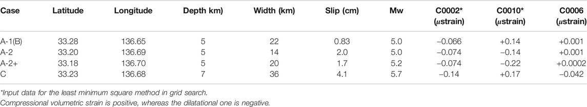
TABLE 5. The best fit fault model for Cases A-C.

The fault location for the best fit model of Case A is shown in Figures 9, 4B, which suggests that Case A can also explain the slip migration toward the updip region under the free constraining condition for the focal depth. Since Figure 4B shows that the epicenters of sVLFE are in the fault model of Case A-2, Case A is also consistent with the timing of the sVLFE activity.

FIGURE 9

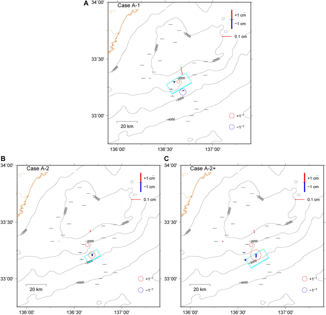
FIGURE 9. Fault model (cyan) for (A) Case A-1, (B) Case A-2, (C) Case A-2+ with the observed volumetric strains (open circle) at C0002 and C0010 and a leveling change at the DONET stations (vertical scale; uplift: red; subsidence: blue). The calculated volumetric strain change at C0002 and C0010 is listed in Table 5. The red vectors represent the horizontal displacement at the GNSS-A stations [Figure 1A (almost 0 for KUM01)]. The contour shows seafloor bathymetry (meter).

In previous SSEs accompanied sVLFE in 2011 and 2015, the rate of pore pressure change at C0010 kept constant until the termination time (Araki et al., 2017). Therefore, we also assume that condition (Case A-2+) as shown by dotted line extended from Case A-2 in Figure 6, where the amount of volumetric strain change at C0010 is −0.22 μstrain as listed in Table 4. The best fit model of Case A-2+ is shown in Figure 9C; Table 5, whose fault geometry is almost the same result as Case A-2.

Case B suggests that the volumetric strain is changed from the Dilation polarity to the Mixed on the way of Case A-2. Since the amount of the volumetric strain change for Case B is almost the same as Case A-1 (Table 4) due to similar rate and period (Figure 6), the best fit model of Case B is also the same as Case A-1. These results suggest that the fault slip migrates from the updip on the way of Case A-2 to intermediate region in Case B, which could not explain the sVLFE activity with the migration toward the updip region (Figure 4) during Case B. Therefore, we conclude that Case B is not acceptable.

The best fit model of Case C is shown in Supplementary Figure S1; Table 5, which has relatively large magnitude with larger slip and wider area covering epicentral locations of C0002 and C0010. This model is expected to have significant volumetric strain change at C0006 (0.042 μstrain in Table 5). However, Figures 3, 6 suggest that the observed one seems no significant signal at C0006 during the event. Therefore, we conclude that Case C is not acceptable.

From these results and t-test in Section Statistical Evaluation of Confidence for Each Case of Pore Pressure Change at C0010, assuming that crustal deformation component of the observed volumetric strain change due to SSE is treated as Case A, we can explain the migration of sVLFE toward the updip region during the SSE reasonably (hereafter, we refer to this event as the SSE in 2020). Since Case A is similar to the time history of pore pressure change for the SSE in 2015, we discuss the characteristics of the SSE in 2020 by comparing with it in the following section.

Summaries and Discussions

First, we discuss the difference of the magnitude between the SSEs in 2020 and 2015. The amplitude of the pore pressure changes for Case A (Table 4) for both C0002 and C0010 sites were smaller than that of the SSE in 2015 (Table 2). The duration of the SSE in 2020 (10 days) was shorter than the SSE in 2015, which was 28 days. As shown in Table 1, five sVLFEs (Mw 2.8 to 3.4) during the SSE in 2020 were detected in 30 h. The total number of sVLFEs (Mw ≧ 3.4) during the SSE in 2015 was more than 20 over 20 days (Takemura et al., 2019), indicating that the cumulative moment magnitude of the sVLFE in 2020 should be smaller than that in 2015. These results suggest that the slip process of the SSE in 2020 is similar to the SSE in 2015 but with a smaller magnitude.

Figure 10 shows the catalog of the pore pressure and the volumetric strain transient at the C0002 and C0010 boreholes with the simplified fault models for the previous SSEs in Table 2 and Case (A-1) to (A-2) in Table 4 applied to the SSE in 2020 occurring between the origin and termination times as listed in Table 3. As depicted in Figure 10; Table 2, all the duration times for the SSEs, except in 2012, were much shorter than the time resolution of the SSE detection from GNSS-A (0.2 years; Yokota and Ishikawa, 2020). We also estimated the onset and the termination time of the SSE in 2020 in 20 min. Owing to the high time resolution, we estimate the slip process of the SSE in 2020 as migration from the intermediate to the updip regions crossing over beneath C0010.

FIGURE 10

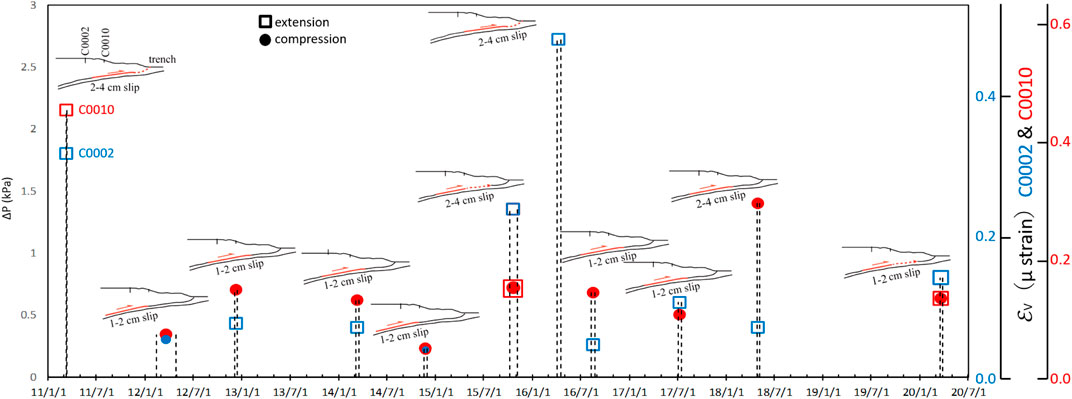
FIGURE 10. Updated summary of the transients in pore pressure (ΔP) and volumetric strain (ε_v) at the C0002 (blue) and C0010 (red) boreholes collated after Araki et al. (2017) (Table 2). The SSE in 2020 is assumed to be Cases A-1 and A-2 in Table 5. The vertical dashed lines indicate the duration of each SSE. The open square and solid circle represent extension and compression, respectively. The schematic cross-sections for each SSE are based on the catalog (Table 2), where the red region represents the slip region.

Because of no significant signal at C0006, we conclude that the slip of the SSE in 2020 did not reach very shallow part of plate interface beneath C0006 as shown in Figure 4B. Figure 4B also shows that sVLFE is not active around the epicentral location of C0006, where the slip amount of the 1944 Tonankai earthquake is relatively small. These results indicate that the volumetric strain just below C0006 might not be accumulated because of stable frictional property near the trench (e.g., Scholtz, 1998), or there is strong coupling enough to refrain from sVLFE activity. This question is to be solved by long-term monitoring at C0006. The results demonstrate that monitoring the pore pressure change is a powerful tool for precisely estimating the region and duration of SSEs. If we estimate the fault model promptly during the pore pressure changes on the basis of our analysis, we can judge the possibility of sVLFE activity in advance of the occurrence.

We could not identify a significant increase in the moment release rate and shorter recurrence interval of the SSE from Figure 10. However, unrecognized SSEs (Katakami et al., 2020) could have possibly been buried in a large noise component. In addition, as mentioned in the Section Estimation of the Onset/Termination Time and the Pore Pressure Change at C0002, there is the temporal decrease of pore pressure during the SSE in 2020 in Figure 5. Because it lasted for several days, which could be explained from the temporal change of slip velocity during the SSE in 2020 rather than the excitation of the local sVLFE or tremors (Kataoka et al., 2004; Barbour 2015) because of the significantly longer period without a comparable increase. Therefore, the development of a noise reduction analysis using other borehole sensors and/or a combination of the nearby hydraulic pressure gauges of DONET would be important in identifying missed SSEs.

The leveling change in all DONET stations is also shown in Figure 9, implying that the expected leveling change was not sufficient for detection (i.e., 0.3 hPa at most). The observed noise level of the DONET pressure gauge was approximately 1–2 hPa (1–2 cm for leveling change) (Suzuki et al., 2016; Takemura et al., 2019). This small leveling change was partly due to low dip angle around the Nankai Trough (e.g., Sugioka et al., 2012).

We discussed the detectability of the horizontal displacement by showing the horizontal displacement of Case A on the seafloor at the GNSS-A stations (Figure 1A) (red arrows, Figure 9). The displacement is expected to be small (0.2 cm at most) if the fault slip is uniform. If the actual fault slip distribution changes spatiotemporally (Fukuda, 2018); thus, the SSE in 2020 can still be detected from other observations, such as GNSS-A (Yokota and Ishikawa, 2020). This will be the focus of our future work.

Data Availability Statement

The datasets presented in this study can be found in online repositories. The names of the repository/repositories and accession number(s) can be found below: http://www-solid.eps.s.u-tokyo.ac.jp/∼sloweq/https://join-web.jamstec.go.jp/join-portal/doi:10.17598/NIED.0008.

Author Contributions

KA estimated the pore pressure change, onset, and termination time of the SSE in 2020. TI estimated the fault model of the Updip region for the SSE in 2020. MN estimated the focal mechanisms of the sVLFEs. TK also checked the pore pressure change independently as double check. EA led the DONET system installation. EA, TK, and YM installed the borehole observatories. TH, NT, and SK commented on improving the manuscript. TK, KS, and KS installed the real-time monitoring system of borehole observatory and DONET, making some figures automatically. SY and TN compiled the SSE catalog.

Funding

This work was partly supported by the Japan Society for the Promotion of Sciences (JSPS), Grant-in-Aid for Scientific Research (KAKENHI) Grant Number JP16H06477, JP17K19093, JP19H02411, and JP20H02236.

Conflict of Interest

The authors declare that the research was conducted in the absence of any commercial or financial relationships that could be construed as a potential conflict of interest.

Acknowledgments

Generic Mapping Tools (Wessel et al., 2013) was used to create figures. The authors would like to thank reviewers for their helpful comment to improve our manuscript, and Editor Keiichi Tadokoro for his expeditious handling.

Supplementary Material

The Supplementary Material for this article can be found online at: https://www.frontiersin.org/articles/10.3389/feart.2020.600793/full#supplementary-material.

References

Araki, E., Saffer, D. M., Kopf, A. J., Wallace, L. M., Kimura, T., Machida, Y., et al. (2017). Recurring and triggered slow-slip events near the trench at the Nankai Trough subduction megathrust. Science 356, 1157–1160. doi:10.1126/science.aan3120

PubMed Abstract | CrossRef Full Text | Google Scholar

Ariyoshi, K., Matsuzawa, T., Ampuero, J.-P., Nakata, R., Hori, T., Kaneda, Y., et al. (2012). Migration process of very low-frequency events based on a chain-reaction model and its application to the detection of preseismic slip for megathrust earthquakes. Earth Planets Space 64, 693–702. doi:10.5047/eps.2010.09.003

CrossRef Full Text | Google Scholar

Ariyoshi, K., Nakata, R., Matsuzawa, T., Hino, R., Hori, T., Hasegawa, A., et al. (2014a). The detectability of shallow slow earthquakes by the Dense Oceanfloor Network system for Earthquakes and Tsunamis (DONET) in Tonankai district, Japan. Mar. Geophys. Res. 35, 295–310. doi:10.1007/s11001-013-9192-6

CrossRef Full Text | Google Scholar

Ariyoshi, K., Matsuzawa, T., Hino, R., Hasegawa, A., Hori, T., Nakata, R., et al. (2014b). A trial derivation of seismic plate coupling by focusing on the activity of shallow slow earthquakes. Earth Planets Space 66, 55. doi:10.1186/1880-5981-66-55

CrossRef Full Text | Google Scholar

Barbour, A. J. (2015). Pore pressure sensitivities to dynamic strains: observations in active tectonic regions. J. Geophys. Res. Solid Earth 120, 5863–5883. doi:10.1002/2015JB012201

CrossRef Full Text | Google Scholar

Davis, E. E., Becker, K., Wang, K., Obara, K., Ito, Y., and Kinoshita, M. (2006). A discrete episode of seismic and aseismic deformation of the Nankai Trough subduction zone accretionary prism and incoming Philippine Sea plate. Earth Planet Sci. Lett. 242, 73–84. doi:10.1016/j.epsl.2005.11.054

CrossRef Full Text | Google Scholar

Dragert, G., Wang, K., and James, T. S. (2001). A silent slip event on the deeper Cascadia subduction interface. Science 292, 1525–1528. doi:10.1126/science.1060152

PubMed Abstract | CrossRef Full Text | Google Scholar

Earthquake Research Committee of the Headquarters for Earthquake Research Promotion (2013). Long-term evaluation of nankai trough earthquake activity. 2nd Edition. Available at: http://www.jishin.go.jp/main/chousa/13may_nankai/nankai2_shubun.pdf (Accessed October 28, 2020).

Google Scholar

Fukuda, J. (2018). Variability of the space‐time evolution of slow slip events off the Boso Peninsula, central Japan, from 1996 to 2014. J. Geophys. Res. Solid Earth 123, 732–760. doi:10.1002/2017JB014709

CrossRef Full Text | Google Scholar

Ichinose, G. A., Thio, H. K., Somerville, P. G., Sato, T., and Ishii, T. (2003). Rupture process of the 1944 Tonankai earthquake (Ms 8.1) from the inversion of teleseismic and regional seismograms. J. Geophys. Res. 108, 2497. doi:10.1029/2003JB002393

CrossRef Full Text | Google Scholar

Ide, S., Beroza, G. C., Shelly, D. R., and Uchide, T. (2007). A scaling law for slow earthquakes. Nature 447, 76–79. doi:10.1038/nature05780

PubMed Abstract | CrossRef Full Text | Google Scholar

Ishikawa, T., Yokota, Y., Watanabe, S., and Nakamura, Y. (2020). History of on-board equipment improvement for GNSS-A observation with focus on observation frequency. Front. Earth Sci. 8, 150. doi:10.3389/feart.2020.00150

CrossRef Full Text | Google Scholar

Ito, Y., Obara, K., Shiomi, K., Sekine, S., and Hirose, H. (2007). Slow earthquakes coincident with episodic tremors and slow slip events. Science 315, 503–506. doi:10.1126/science.1134454

PubMed Abstract | CrossRef Full Text | Google Scholar

Kaneda, Y., Kawaguchi, K., Araki, E., Matsumoto, H., Nakamura, T., Kamiya, S., et al. (2015). “Development and application of an advanced ocean floor network system for megathrust earthquakes and tsunamis?,” in Seafloor observatories,(Chichester, United Kingdom: Springer Praxis Books), 643–663. doi:10.1007/978-3-642-11374-1_25

CrossRef Full Text | Google Scholar

Kano, M., Aso, N., Matsuzawa, T., Ide, S., Annoura, S., Arai, R., et al. (2018). Development of a slow earthquake Database. Seismol Res. Lett. 89, 1566–1575. doi:10.1785/0220180021

CrossRef Full Text | Google Scholar

Katakami, S., Kaneko, Y., Ito, Y., and Araki, E. (2020). Stress sensitivity of instantaneous dynamic triggering of shallow slow slip events. J. Geophys. Res. Solid Earth 125, e2019JB019178. doi:10.1029/2019JB019178

CrossRef Full Text | Google Scholar

Kataoka, S., Ueda, K., Okamoto, A., and Hasegawa, M. (2004). “Observed dynamic pore pressure during earthquake in saturated rock,” in 13th World conference on earthquake engineering vancouver, Vancouver, BC, August 1–6, 2004, 3470.

Google Scholar

Kawaguchi, K., Kaneko, S., Nishida, T., and Komine, T. (2015). “Construction of the DONET real-time seafloor observatory for earthquakes and tsunami monitoring,” in Seafloor observatories,(Chichester, United Kingdom: Springer Praxis Books), 211–228. doi:10.1007/978-3-642-11374-1_10

CrossRef Full Text | Google Scholar

Kitada, K., Araki, E., Kimura, T., Kinoshita, M., Kopf, A., and Saffer, D. (2013). “Long-term monitoring at C0002 seafloor borehole in Nankai Trough seismogenic zone,” in 2013 IEEE international underwater technology symposium (UT), Tokyo, March 5–8, 2013(IEEE), 1–3. doi:10.1109/UT.2013.6519882

CrossRef Full Text | Google Scholar

Maeda, T., Obara, K., Shinohara, M., Kanazawa, T., and Uehira, K. (2015). Successive estimation of a tsunami wavefield without earthquake source data: a data assimilation approach toward real‐time tsunami forecasting. Geophys. Res. Lett. 42, 7923–7932. doi:10.1002/2015GL065588

CrossRef Full Text | Google Scholar

Matsuzawa, T., Hirose, H., Shibazaki, B., and Obara, K. (2010). Modeling short- and long-term slow slip events in the seismic cycles of large subduction earthquakes. J. Geophys. Res. 115, B12301. doi:10.1029/2010JB007566

CrossRef Full Text | Google Scholar

Murotani, S., Shimazaki, K., and Koketsu, K. (2015). Rupture process of the 1946 Nankai earthquake estimated using seismic waveforms and geodetic data. J. Geophys. Res. 120, 5677–5692. doi:10.1002/2014JB011676

CrossRef Full Text | Google Scholar

Nakamura, T., Takenaka, H., Okamoto, T., Ohori, M., and Tsuboi, S. (2015). Long-period ocean-bottom motions in the source areas of large subduction earthquakes. Sci. Rep. 5, 16648. doi:10.1038/srep16648

PubMed Abstract | CrossRef Full Text | Google Scholar

Nakano, M., Hori, T., Araki, E., Kodaira, S., and Ide, S. (2018). Shallow very-low-frequency earthquakes accompany slow slip events in the Nankai subduction zone. Nat. Commun. 9, 984. doi:10.1038/s41467-018-03431-5

PubMed Abstract | CrossRef Full Text | Google Scholar

Nakano, M., Hori, T., Araki, E., Takahashi, N., and Kodaira, S. (2016). Ocean floor networks capture low-frequency earthquake event. Eos. doi:10.1029/2016EO052877

CrossRef Full Text | Google Scholar

National Research Institute for Earth Science and Disaster Resilience (2019). NIED DONET. Tokyo: National Research Institute for Earth Science and Disaster Resilience. doi:10.17598/NIED.0008

CrossRef Full Text | Google Scholar

Nishikawa, T., Matsuzawa, T., Ohta, K., Uchida, N., Nishimura, T., and Ide, S. (2019). The slow earthquake spectrum in the Japan Trench illuminated by the S-net seafloor observatories. Science 365, 808–813. doi:10.1126/science.aax5618

PubMed Abstract | CrossRef Full Text | Google Scholar

Obara, K., and Kato, A. (2016). Connecting slow earthquakes to huge earthquakes. Science 353, 253–257. doi:10.1126/science.aaf1512

PubMed Abstract | CrossRef Full Text | Google Scholar

Obara, K. (2002). Nonvolcanic deep tremor associated with subduction in southwest Japan. Science 296, 1679–1681. doi:10.1126/science.1070378

PubMed Abstract | CrossRef Full Text | Google Scholar

Okada, Y. (1992). Internal deformation due to shear and tensile faults in a half-space. Bull. Seismol. Soc. Am. 82, 1018–1040.

Google Scholar

Saffer, D., Kopf, A., and Toczko, S. (2017). “The expedition 365 scientists,” in Proceedings of the international ocean discovery program, 365, November 23, 2017. Available at: publications.iodp.org (Accessed November 23, 2017). doi:10.14379/iodp.proc.365.103.2017

CrossRef Full Text | Google Scholar

Scholtz, C. H. (1998). Earthquakes and friction laws. Nature 391, 37–42. doi:10.1038/34097

CrossRef Full Text | Google Scholar

Schwartz, S. Y., and Rokosky, J. M. (2007). Slow slip events and seismic tremor at circum–pacific subduction zones. Rev. Geophys, 45, RG3004. doi:10.1029/2006RG000208

CrossRef Full Text | Google Scholar

Sugioka, H., Okamoto, T., Nakamura, T., Ishihara, Y., Ito, A., Obana, K., et al. (2012). Tsunamigenic potential of the shallow subduction plate boundary inferred from slow seismic slip. Nat. Geosci. 5, 414–418. doi:10.1038/ngeo1466

CrossRef Full Text | Google Scholar

Suzuki, K., Nakano, M., Takahashi, N., Hori, T., Kamiya, S., Araki, E., et al. (2016). Synchronous changes in the seismicity rate and ocean-bottom hydrostatic pressures along the Nankai Trough: a possible slow slip event detected by the Dense Oceanfloor Network system for Earthquakes and Tsunamis (DONET). Tectonophysics 680, 90–98. doi:10.1016/j.tecto.2016.05.012

CrossRef Full Text | Google Scholar

Takemura, S., Noda, A., Kubota, T., Asano, Y., Matsuzawa, T., and Shiomi, K. (2019). Migrations and clusters of shallow very low frequency earthquakes in the regions surrounding shear stress accumulation peaks along the Nankai Trough. Geophys. Res. Lett. 46, 11830–11840. doi:10.1029/2019GL084666

CrossRef Full Text | Google Scholar

To, A., Obana, K., Sugioka, H., Araki, E., Takahashi, N., and Fukao, Y. (2015). Small size very low frequency earthquakes in the Nankai accretionary prism, following the 2011 Tohoku-Oki earthquake. Phys. Earth Planet. In. 245, 40–51. doi:10.1016/j.pepi.2015.04.007

CrossRef Full Text | Google Scholar

Wallace, L. M., Araki, E., Saffer, D., Wang, X., Roesner, A., Kopf, A., et al. (2016). Near-field observations of an offshore Mw 6.0 earthquake from an integrated seafloor and subseafloor monitoring network at the Nankai Trough, southwest Japan. J. Geophys. Res. Solid Earth 121, 8338–8351. doi:10.1002/2016JB013417

CrossRef Full Text | Google Scholar

Wessel, P., Smith, W. H. F., Scharroo, R., Luis, J., and Wobbe, F. (2013). Generic mapping tools: improved version released. Eos Trans. AGU 94 (45), 409. doi:10.1002/2013EO450001

CrossRef Full Text | Google Scholar

Wiseman, K., and Bürgmann, R. (2011). Stress and seismicity changes on the sunda megathrust preceding the 2007 M_w 8.4 earthquake. Bull. Seismol. Soc. Am. 101 (1), 313–326. doi:10.1785/0120100063

CrossRef Full Text | Google Scholar

Yokota, Y., and Ishikawa, T. (2020). Shallow slow slip events along the Nankai Trough detected by GNSS-A. Sci. Adv. 6, eaay5786. doi:10.1126/sciadv.aay5786

PubMed Abstract | CrossRef Full Text | Google Scholar