Model-Based Forecasting of Agricultural Crop Disease Risk at the Regional Scale, Integrating Airborne Inoculum, Environmental, and Satellite-Based Monitoring Data

Introduction

Crop diseases have the potential to cause devastating epidemics that threaten the world's food supply and vary widely in their dispersal pattern, prevalence, and severity (Chakraborty and Newton, 2011). Diseases like stripe rust (Puccinia striiformis f. sp. tritici) (Pst) and fusarium head blight (Fusarium graminearum) (FHB) on wheat, and powdery mildew (Erysiphe necator) on grapes, to highlight just a few, cause major crop losses globally (Hovmøller, 2001; Carisse et al., 2009; Haran et al., 2010; Newberry et al., 2016). Plant breeding to increase host resistance remains the primary approach for managing diseases and to help sustainable agricultural yields, as crop breeding networks that deploy resistance genes decrease the likelihood that pathogens will overcome resistance (Ojiambo et al., 2017). Nonetheless, despite the introduction of crop cultivars/varieties with higher resistance, new disease races, with increased virulence, continue to emerge. Environmental conditions affect resistance gene performance, but the basis for this is poorly understood (Bryant et al., 2014). Moreover, environmental drivers and pressures are increasing in their influence over agroecosystems; climate change and variability is raising temperatures and lengthening growing seasons, especially in northern climates (Canada) or temperate zones (Australia), producing more days without frost, and more intense heatwave and rainfall events. Disease dynamics itself involves a complex interaction between a host, a pathogen, and their environment, representing one of the largest integrated risks facing the long-term sustainability of agriculture. Genetic factors (e.g., emergence of new diseases and of new races), environmental-driven influence (e.g., global climate change impacts on disease spread), and management-intervention driven agroecosystem interactions (e.g., crop breeding and monitoring technologies) are all important considerations in disease risk mitigation.

The cost of pesticides (e.g., fungicides, insecticides, herbicides) is a substantial burden for growers—with substantial uncertainty involved in deciding when and how much to apply to commercial fields, especially as multiple diseases often affect crops at the same time. Currently, when monitoring their fields for disease, growers often rely on simple, visual identification, assessing severity using standard area diagrams (SADs), disease progress (AUDPC) curves, and weather/forecast conditions (Contreras-Medina et al., 2009; Nopsa and Pfender, 2014; Ojiambo et al., 2017). Pesticides are then applied either preventatively, or even if no disease is detected, on a calendar-based schedule, based on perceived risk (Carisse et al., 2009). This approach is, however, limited in its ability to detect and control disease. Pesticide application must generally occur during the early stages of epidemics, and at sufficient rates. Over-application is costly and creates added selection pressure for more pesticide tolerant strains, while under-application may also be cost-prohibitive in regions where expected yield is lower (Chen, 2007). Moreover, high pesticide concentrations are not only costly, but are also associated with detrimental environmental and human health impacts (Newlands, 2016). Reducing pesticide use is a major focus of global agricultural sustainability efforts (Nicolopoulou-Stamati et al., 2016). The effectiveness of applications are also highly dependent on timing, stage of disease progression, and the strength and directionality of micro- and meso-scale wind currents (Meyer M. et al., 2017).

Integrated Pest Management (IPM) is the deployment of a variety of methods of pest control designed to complement, reduce, or replace the application of synthetic pesticides. It involves regular monitoring, use of decision thresholds, combining approaches for targeted pesticide management and substitution to broader agroecosystem considerations (Pretty and Bharucha, 2015). For a comprehensive global overview of the history, programs, and adoption of IPM programs around the world, readers are referred to Peshin et al. (2009). They highlight problems with assessing the adoption and success of IPM programs and how pesticide use has not consistently decreased in the majority of programs, despite reduction of pesticide use being one of their primary goals. Here predictive models may not only enable better program assessment and adoption, but also help to identify how to optimize changes in the timing and application of pesticides (e.g., fungicides) in time and space to reduce pesticide use where predicted disease risk is sufficiently low. Disease prediction models using advanced statistical methods (e.g., artificial neural networks) integrating weather and aerobiological monitoring data have been successfully developed and validated for Ganoderma spp. and white blister on Brassica crops (Brassica spot^TM) (Minchinton et al., 2013; Sadyś et al., 2016). Such prediction models need to be adapted and extended for other crop diseases and then integrated into operational IPM programs. For many IPM programs, there is a crucial need to develop and involve a more reliable and effective approach (i.e., analytical framework) for managing disease risk that establish relationships between the amount of airborne inoculum and disease development, combined use of models that integrate theoretical knowledge on crop (host) growth, disease (pathogen) development, and environmental influences; alongside data from disease monitoring, climate/weather, and other explanatory variables for assessing and predicting disease (Juroszek and von Tiedemann, 2013; Ojiambo et al., 2017). Past efforts have been hindered by sparse spatial data, limited use of field monitoring technology, and a need for greater integration and quantification. Past efforts have also concentrated mainly on understanding the physical and biological mechanisms of plant (crop) pathogen spore dispersal linked disease development, outbreaks and spatial epidemic patterning and spread. Improved detection of new airborne inoculum, weather, and satellite-based technology, however, provide new opportunities for combining disease monitoring data with predictive models. This has the potential to improve the timeliness, effectiveness and foresight for controlling crop diseases, while minimizing crop loss (Isard et al., 2011; Devadas et al., 2015; West and Kimber, 2015; Mahlein, 2016).

In a recent review of modeling the impact of climate on crop disease, improvements in measuring the uncertainty of climate change projected impacts using multi-model ensembles are highlighted. This synthesis identifies the need to explore other sources of uncertainty inherent in disease models that still remain unexplored and unreported (Newberry et al., 2016). They articulate the crucial need to investigate crop disease dynamics at the landscape spatial scale, across a broader range of crops and pathogens. This study also identifies the need for new frameworks and models to improve the ability of models to predict impacts of climate change on crop diseases for guiding the planning of climate change adaptation strategies to ensure future food security. Because disease patterns can change in unintended ways when interventions take place across spatially heterogeneous landscapes, Newberry et al. (2016) articulate five key challenges for advancing models: (1) flexibility and accuracy, (2) interaction and contact assumptions and statistical representation, (3) how to define and estimate a critical threshold of transmissibility, while recognizing a mixture of infection types under changing susceptibility, (4) how to model disease dynamics that depends on long-distance interaction (e.g., air transmission via wind trajectories with deposition via rainfall events), and, (5) identifying the natural scale (i.e., operational resolution) for modeling (and forecasting) transmission and interaction, and how this relates to the scale at which intervention is most effective, recognizing that different sources of data are typically available at different scales (Riley et al., 2015).

Model uncertainty and reliability remain two major issues challenging the development of more robust and effective quantitative approaches for disease management. To address these aspects requires an integrated model-based framework and statistical approach that can integrate new types of data, model spatial and temporal dependence and interaction, quantify uncertainties, evaluate multiple scenarios, and bridge empirical-theory knowledge gaps (Held et al., 2004; Contreras-Medina et al., 2009; Haran et al., 2010; Savage and Renton, 2014; Kouadio and Newlands, 2015; Riley et al., 2015; Newlands, 2016; Höhle et al.,, 2017; Ojiambo et al., 2017). Dennis (1987) derived a simple, multivariate regression-based model of Pst disease infection based on air temperature and surface wetness period. Incorporating Monte-Carlo simulation to model uncertainty, El Jarroudi et al. (2017) further incorporated the Dennis disease infection model into a threshold-based weather model to guide fungicide applications for Pst. They show that an optimal combination of high humidity (>92%), temperature (4–16^oC) for at least 4 consecutive hours was sufficient to cause an epidemic. Audsley et al. (2005) developed a simulation model integrating it within the Decision Support System for Arable Crops (DESSAC) system that uses a genetic algorithm for the selection of fungicide spray plans (Parsons and Te Beest, 2004; Audsley et al., 2005), integrating major risk variables for pathogen (i.e., inoculum source and transfer), host (cultivar-specific resistance, leaf age, nitrogen uptake), and weather conditions (temperature, rain, humidity, wind), Using the simple, multiple regression modeling approach, Kuang et al. (2013) demonstrated a model-based, operational prediction system for wheat stripe rust that integrates geospatial and internet/networking technology to enable multiple users to interact, share data, automate, and update model design, combining regional predictions and testing statistical significance. The inter-comparison of assumptions (models), spatial resolution and uncertainty (climate datasets), spatial correlation/dependence of host-pathogen-environmental interaction, and its effect on model performance and forecast accuracy is lacking.

In this paper, an integrated modeling framework to forecast disease risk is proposed. The feasibility of model-based, operational disease risk forecasting is investigated, using data available for wheat stripe (yellow) rust (Puccinia striiformis f.sp. tritici) (hereafter, Pst) fungal disease within southern Alberta, Canada. Two candidate, stochastic models are evaluated; a simpler, site-specific model, and a more complex, transmission model. These models are calibrated using airborne inoculum data by a Burkard cyclone spore collector, for the first time. In addition, satellite measurements of major disease risk variables (i.e., canopy temperature and liquid water on the canopy surface) are integrated. The ability of these models to reproduce an observed infection pattern is tested using two climate datasets with different spatial resolution—a reanalysis dataset (~55 km) and a weather station network township-aggregated data (~10 km).

Materials and Methods

Integrated Modeling Approach

The integrated framework was designed to take into account major aspects and considerations involved in operational model-based forecasting of crop disease at the regional-scale (Figure 1). This approach combines data on host, pathogen and environment, and models to capture different aspects of disease dynamics under different assumptions. In this figure, starting and end points are shown with respect to seasonal disease progression. Boxes represent model components—dashed boxes are disease aspects not considered in the current modeling. Full boxes are those that are currently considered. This design is a prototype, and while not exhaustive of all general and pathogen-specific aspects, is based on published scientific studies, evidence, and in consultation with several expert AAFC/Canadian pathologists. This design supports feasibility testing, involving the evaluation of different models, datasets, and forecast metrics. The framework integrates threshold-based infection and multivariate spatial assumptions, extending previous approaches to include a broader, more representative set of disease dynamic parameters, climate covariates, and assumptions on disease-climate interaction and spatial dependence. Its component-wide structure permits scaling-up from homogeneous to heterogeneous assumptions, whereby a region is divided into smaller subregions, with transmission assumed to occur between them and a calibrated model used to capture their specific disease dynamics, susceptibility, incidence, and risk. Further details of the model input and output parameters and variables are provided for a non-spatial/site-specific (CLR) and spatial model (hhh4) formulation in this section.

FIGURE 1

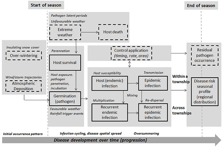
Figure 1. A prototype integrated, model-based framework for forecasting disease risk. Risk components for the major disease progression stages (i.e., immigration, deposition, germination, infection, incubation/residency, multiplication, re-dispersal, perennation) are included, alongside major risk variables, e.g., weather trigger events and conditions, host exposure and susceptibility, pathogen survival, residency, latency, endemic infection, cycling, epidemic transmission and dispersal, and evolved virulence associated with the risk of resistance breakdown in the field (i.e., finer subregions compared to the ROI). Full boxes are components of the framework that are considered in the current disease risk modeling, while dashed boxes will be considered in future extended modeling.

Wheat Stripe Rust Disease

Stripe (yellow) rust (Pst) is a prevalent fungal disease in all wheat (Triticum aestivum) growing regions around the world, occurring in most production zones having cool and moist weather conditions during the growing season (Chen et al., 2014). This disease has the potential to cause devastating outbreaks/severe epidemics that threaten the world's wheat supply and, in turn, global food security, as 88% of the world's wheat production of 760 million metric tons (~$185 USD/mt or $140.6 billion USD in 2017/18) is susceptible (World Bank Group, 2017; Food and Agriculture Organization of the United Nations (FAO), 2018). This fungus (a wind-dispersed, obligate biotroph that only infects and survives in a living host) has yellow urediniospores during its asexual infection cycle and is able to disperse over long distances across continents. It is also adapting and overcoming resistance genes via rapid stepwise evolution (Lei et al., 2017; Schwessinger, 2017). There are different types of resistance depending on host wheat plant growth stages and environment (laboratory or field), such that stripe rust resistances can be separated into all-stage (also called seedling) resistance (ASR) verses adult-plant resistance (APR); greenhouse resistance and field resistance; temperature insensitive resistance verses temperature sensitive resistance; and non-durable resistance vs. durable resistance (Wang and Chen, 2017). With the constant evolution of new rust strains, and their adaptation to higher temperatures, consistent and durable disease resistance is a key challenge. The dual/split application of fungicide, with half rates applied early and later, can reduce disease intensity (AUDPC metric) close to that of a single, full application, based on field trials of fungicide effectiveness (Braithwaite, 1998). Crop rotation likely does not prevent the spread of Pst, given its rate of spread is so fast across large areas (Xi et al., 2015). Nonetheless, delayed planting, reduced irrigation, avoidance of excessive nitrogen use, and elimination of volunteer and grass plants can reduce stripe rust severities—but these cultural practices are often not profitable, conflict with conservation farming, and/or reduce yield potential (Chen, 2007). A consideration of host resistance, pathogen survival and dynamics, alongside best management or cultural practices, enabling farmers to use fungicides more judicially, is a long-term, ultimate need and goal to minimize the risk of this disease (Xi et al., 2015).

Most areas of the United States are not suitable for Pst survival in both summer and winter, and only the Pacific Rim states (California, Oregon, and Washington) have favorable areas where the disease survives in summer and winter (i.e., oversummering and overwintering), based on summer/winter survival indices linked to climate conditions (Sharma-Poudyal, 2012; Sharma-Poudyal et al., 2014). The major source of stripe rust inoculum for Alberta (Western Canada) is considered to be from this Pacific Northwest region (hereafter PNW) (Xi et al., 2015). Pst occurrence is generally associated with higher elevations, northern latitudes or cooler years (Newberry et al., 2016). For regions north of latitude 40°N, it infects both winter wheat and spring wheat (winter wheat is generally more susceptible than spring wheat), surviving in cool summers, with hot summers substantially decreasing the chance of its survival, and severe winters preventing its survival (Xi et al., 2015). Pst development becomes dormant for longer durations (slower cycle time) as night-time temperatures cool. In this way, indices based on average daily mean temperatures may overestimate infection risk, especially in early spring and late summer, when cooler nights are more frequent. Because different races can infect different wheat varieties/cultivars having different resistance to the pathogen, the reaction of different resistance genes on selected host varieties/cultivars (differentials) is used to determine the “race spectrum” for a given pathogen population (e.g., within a single field). As with most other wheat-growing regions, urediniopores (asexual cycle) are the only inoculum source for the initial and recurrent infection of wheat, with an infection cycle time that varies through the growing season. New and older rust isolates (i.e., pathogen isolated in field samples that are geographically or location specific) within Western Canada have similar urediniospore rates of germination, occurring between 2 and 20°C, and highest/optimal close to 5°C, with cooler temperatures favoring spore germination (Tran and Kutcher, 2015). While Pst outbreaks have been documented in Alberta since 1925, the variable virulence of Pst has enabled it to overcome the resistance of wheat cultivars, with increasing epidemics occurring in the 1990s, whereby the older population of races (i.e., pathotypes) in the United States have been replaced by a new population since 2000 with germination occurring at higher temperatures between (16–18°C) and being more tolerant of higher summer temperatures (Chen, 2010; Xi et al., 2015).

Warm chinook winds create milder winter weather conditions across southern Alberta and change snow cover. Snow cover is beneficial to urediniospore survival during the winter, whereby areas in the vicinity of Olds are more conducive for spore survival than areas near Lethbridge. This enables Pst to overwinter in this region, and cause outbreaks in early spring when the weather is cool and wet (Conner et al., 1988; Phillips and Newlands, 2011; Xi et al., 2015). Significant snow cover (>7.6 cm) has an insulative effect, enabling Pst to infect wheat within 4–6 h and survive at temperatures down to −10°C. With no snow cover and with temperatures less than −5°C, Pst goes dormant (Sharma-Poudyal et al., 2014). Newer isolates have thus adapted to warmer temperatures and have higher germination rates at higher temperatures than older isolates. The definition of latent period is the approximate time taken for an infection to result in new spores and is temperature-dependent; within an optimal temperature range between 12 and 20°C. Latent period is 10–14 days (Anonymous, 2018) and is cultivar-dependent; a susceptible cultivar AC Bellatrix of red winter wheat (first released by AAFC in Lethbridge in 1999) was shorter at higher temperature for new isolates, with a higher disease intensity over time for new isolates, compared to older ones (i.e., measured as the area under the disease progress curve or AUDPC) (Tran and Kutcher, 2015). This evidence supports the hypothesis that new stripe rust populations continue to adapt to warming temperatures, with increased aggressiveness and explains its expansion into Alberta, including other Canadian Prairie Provinces (i.e., Western Saskatchewan). For Eastern Saskatchewan and Manitoba the source of Pst is from the Mississippi Valley, recent field surveys conducted during July, August, and September 2016 on winter and spring wheat indicate that Pst is found with varying levels of infection depending on spatial location. Winter wheat lines, depending on location and cultivar, can have upwards of 70% infection (2016 Cereal Disease Situation Report, Western Committee on Plant Disease, WCPD. Unpubl.). A recent global analysis of Pst outbreaks involving 887 genetically diverse isolates across 35 countries (2009–2005) reveals that a few, highly divergent genetic races are driving its epidemics and that its populations are being largely shaped by invasion across geographical areas (Ali et al., 2017). With such high epidemic potential, there is greater urgent need for improved predictability of its emergence and dynamics.

Study Region (Southern Alberta, Canada)

The region of interest (hereafter, ROI) is southern Alberta (within Western Canada), a major area of agricultural production with a growing season of about 123 days (May-August). Wheat is the largest crop, followed by barley and canola. Crops are irrigated in this region due to reduced rainfall (semi-arid conditions: 300–450 mm/year). In 2015, adverse weather conditions (i.e., dry spring, low night-time temperatures and frost in fields, hot summer with limited moisture) led to poor growing conditions with yields being lower than long term averages. It first affects winter wheat fields before spreading into spring wheat, as winter wheat (e.g., AC Bellatrix and Radiant varieties) is direct-seeded in early September and harvested several weeks earlier than spring wheat the next year. Pst immigrates into this region from the south (i.e., PNW and areas in the vicinity of Portland, Oregon), as well as, from the north where it overwinters in central Alberta. Backward, diagnostic trajectories (5-day time frames) using analyzed wind fields, indicate that Pst within the NWR of the United States is the main Pst source region for southern Alberta, Canada (AAFC Cereal Rust/Wind Trajectory Event Update Report (Summer 2015) by Turkington et al. Unpubl.). Also, forward, prognostic trajectories using NOAA's HYSPLIT model (April-May, 1995) and forecast wind fields (discrete fields 700–850 hPa) having starting points within the PNW region (vicinity of Portland, Oregon USA) show an immigration zone for high potential for spore dispersion into southern Alberta (not included here for brevity, Newlands unpubl.). These simulations use archived (2-hourly) weather data from Regional Analysis and Forecast System (RAFS)'s Nested Grid Model (NGM) (US National Centers for Environmental Prediction, NCEP). The atmospheric deposition of spores onto the ground still needs to be accounted for, using models such as the one developed by Chamecki et al. (2012) to know more accurately where and when they fall.

Airborne inoculum sample data (weekly, June-October) was obtained for 2015 at Lethbridge (Fairfield site: N 49° 42.493/ W 112° 41.738) from the first year of sampling (Figure 2) with sticky microscope slides placed on a Burkard cyclone spore collector. This is considered a passive method of spore trapping/collection, instead of active sampling of the air. The slides were attached on the cap of the Burkard cyclone instrument, just below the collection orifice, so that the slide was always facing the prevailing wind (i.e., 180° incidence angle). Double-sided adhesive tape (#M Scotch^® Removable Poster Tape 3/4′ (199 mm) wide, clear) was used. The adhesive tape covered almost the whole translucid surface of the slide, covering an area of 19 × 50 mm. The slides were kept inside a slide box at room temperature for a few days until they were analyzed under a light microscope (Laroche et al., 2018). While it could have been located anywhere in the study region for the entire growing season, it was fixed in its location in an agricultural field (Fairfield) located in Lethbridge, given the high Pst visual occurrence historically detected in fields near this site. Microscopy, Polymerase chain reaction (PCR), and multiplex qPCR molecular techniques were used to identify Pst urediniospores and quantify the concentration of spores collected by the cyclone collector instrument (Araujo et al., 2016) (PCR is a technique to make many copies of a specific DNA region in vitro).

FIGURE 2

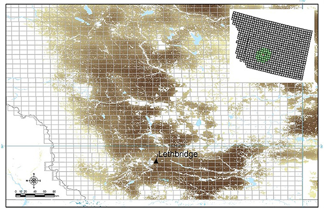
Figure 2. The southern Alberta, Canada region of interest (ROI): The Lethbridge site (located within township TW008R21W4) is indicated; areas where wheat (winter, spring) are grown are indicated (brown) superimposed on a grid of Alberta townships (~10 km). A sub-region of 40 municipalities was selected surrounding the Lethbridge site for model computations (upper inset).

Satellite measurements of major disease risk variables (i.e., canopy temperature and liquid water on the canopy surface) (Laroche et al., 2018), regional-scale climate reanalysis (Kobayashi et al., 2015), and quality-controlled weather station network data (hourly scale), spatially-interpolated to the regional municipality scale were provided by the Alberta Climate Information Service (ACIS) (1961-2016)¹. The ACIS interpolation method linearly weights station-based air temperature estimates of up to 8 closest neighboring stations by inverse-distance, within a correlation radius of 60 km. Precipitation is inversely-weighted by distance (i.e., cube of the inverse distance within a correlation radius of 200 km), with the inverse distance monthly totals redistributed proportionally, relative to the nearest station with a complete monthly record. The JRA-Year Reanalysis (JRA-55) high-resolution, climate reanalysis dataset was used, being among the most sophisticated reanalyses currently available. It also includes pathology-relevant variables with a spatial resolution of 0.55° × 0.55° (~55 km) and 3-hourly (and 6-hourly) temporal resolution for years 1990-2015 (Bebber et al., 2016). Figure 3 compares the distribution of potential disease risk based simply on climate variables (i.e., thresholds in mean daily temperature and humidity range) illustrating how the importance of finer resolution in revealing spatial trends and correlation patterns, and the need to model such spatial impacts to predict disease risk rather than relying on climate threshold-based information alone. Simple thresholds are typically assumed in many current operational, weather-based disease risk forecasting systems, avoiding the use of models with assumptions of pathogen-host-environmental interaction that adds additional uncertainty to risk forecasts. The finer-scale pattern of potential Pst pathogen infection risk revealed across the townships (~10 km) varies considerably from the host (i.e., wheat) distribution pattern, pointing to the need and importance of disease risk modeling to explain and better predict differences in host and pathogen distribution and variability in relation to environmental (e.g., climate) uncertainty (Figure 2). Also, information on fungicide efficacy in relation to spray timing and varietal response for stripe rust control is limited in central Alberta, contributing additional uncertainty (Xi et al., 2015).

FIGURE 3

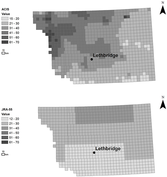
Figure 3. Spatial distribution of potential Pst infection risk between June 17 and Sept 1 in 2015 (in units of total number of growing season days having conditions favorable to infection). The total number of growing season days was based on threshold range of mean daily temperature 3–25^oC, average humidity >57% (ACIS) and hourly canopy moisture >0 (wet days) (JRA-55), illustrating the effect of spatial resolution and importance of capturing spatial dependence (in finer-scale climate data) for improving model-based disease prediction. (ESRI ArcGIS 10.4, Canada Albers Equal Area Conic Projection).

Hourly leaf wetness duration (LWD) and canopy temperature (T_c) data was obtained from the JRA-55 reanalysis dataset. Canopy moisture (kg m⁻²) and temperature (°C) was converted² from the JRA-55 variables named “moisture storage on canopy” (code 223) (m) and “canopy temperature” (code 114) (K) from the ground/land surface forecast fields (fcst_land125) produced every 3 h (at 00, 03, 06, 09, 12, 15, 18, and 21UTC) (Figure 4). Leaf wetness duration (LWD) is highly skewed, with many dry days (Figure 4A). Leaf wetness is the presence of free water on the surface of a crop canopy comprising canopy-intercepted rainfall/fog, irrigation, and dew (dewfall/dew-rise) that forms on leaves where water vapor condenses on a surface; it is triggered when the temperature of a canopy surface drops below the dew point temperature of the surrounding air (Rolandson et al., 2015). In June-Oct of 2015, coinciding with the airborne sampling measurement, the majority of wetness events were below 0.001 m (or 0.10 kg m⁻²) early in the season (June), but increases through the season reaching 0.30–0.35 kg m⁻² at end-of-season (August-Oct) (Figure 4B). There were 54 days with rainfall (of 77 total of airborne sampling in 2015). Canopy temperature showed considerable variability through the 2015 growing season (Figure 4C).

FIGURE 4

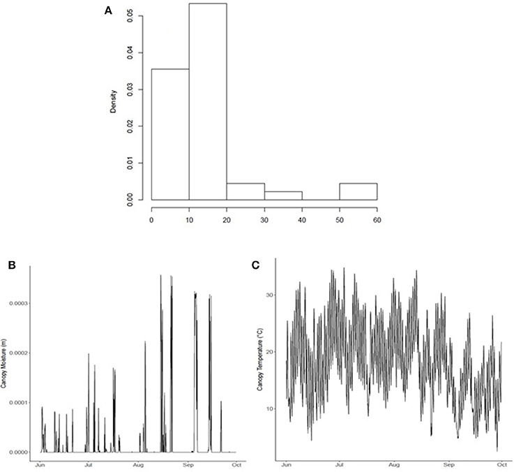
Figure 4. (A) Growing season wetness duration (h) distribution, (B) canopy wetness (m), and (C) temperature (^oC) within the modeled ROI comprising 40 townships within the 2015 growing season, surrounding the Lethbridge site.

CLR Model (Site-Specific)

A site-specific model was first evaluated in predicting Pst disease. This model has previously been used to predict disease risk and a historical 2008-2011 outbreak of Coffee Leaf Rust (CLR, Hemileia vastatrix) in Colombia (Bebber et al., 2016) (hereafter, CLR model). The CLR model assumes infection by germinated fungal spores occurring on leaves that are wet for longer than a critical leaf wetness duration (W_crit or LWD_crit) and specifies a temperature response function [(Yan and Hunt, 1999) Type] of germination and infection based on pathogen-specific minimum, maximum and optimum temperature (θ_min, θ_opt, θ_max). Sensitivity analysis of a generic fungal model for Pst using these variables lends further support for their use in predicting Pst disease dynamics (Bregaglio et al., 2012). The model assumes: temperature is assumed constant over each hourly interval, an equal size of new spore cohorts that being germinating at the start of each wet hour, and no germination during dry periods, with no neighbor infections. The process of spore germination and appressoria formation (i.e., infection) over time is modeled as a Weibull-distributed survival process. This generates a cumulative hazard function having germination and infection processes that are time-varying and random, with rates that are greatest at θ_opt and decline to zero outside of the temperature range (θ_min, θ_max). Disease development is thus assumed to be dormant until the temperature moves back within the required range. The CLR model was implemented using validated R code [(Bebber et al., 2016; R Core Team, 2017) (includes supplement and example R code)] with the critical wetness, temperature-response, and germination/infection process (Weibull-distribution) parameters estimated for Pst, using the JRA-55 reanalysis 3-hourly climate data.

hhh4 Model (Spatial)

The hhh4 spatio-temporal endemic-epidemic model having spatial dependence assumptions was selected to compare with the CLR site-specific model predictions. This model has been implemented in the surveillance R package (Held and Paul, 2012; Paul and Meyer, 2016; Meyer S. et al., 2017). Separate runs of the model using JRA-55 reanalysis (~55 km), ACIS station-based township (~10 km) climate data as input, and both datasets combined, were performed to benchmark the effect of the spatial resolution of input climate data on disease model accuracy. The hhh4 model is a multivariate time-series model for disease incidence, Y_it involving multiple, geographical sub-regions (e.g., units of townships or fields), i = (1,…,I), across multiple time periods t = (1,…,T). It assumes a negative-binomial (i.e., clustered) distribution of spore counts, with an additive mean (Meyer S. et al., 2017),

$\begin{array}{ll}{\mu }_{it}=e_{it}\nu {}_{it}+{\lambda }_{it}{Y}_{i,t-1}+{\varphi }_{it}{\displaystyle {\sum }_{j\ne i}{w}_{ji}{Y}_{j,t-1}}& (1)\end{array}$

and the over-dispersion parameter, ψ_i. The additive mean μ_it consists of an endemic (e_it ν_it) and epidemic $({\lambda }_{it}{Y}_{i,t-1}+{\varphi }_{it}{\displaystyle {\sum }_{j\ne i}{w}_{ji}{Y}_{j,t-1}})$ component, where e_it is the expected counts (i.e., a multiplicative offset to the endemic mean ν_it). The epidemic component consists of two autoregressive spatial effects, namely: disease reproduction within region i, and a neighborhood or spatial-temporal interaction effect involving spore transmission to other region j. The disease endemic and epidemic contributions can be assumed identical across regions, vary within each region, random, or correlated between regions, by representing them as log-linear functions having intercept, α_i and associated predictor variables, whereby,

$\begin{array}{ll}\log \left({\nu }_{it}\right)={\alpha }_i^{(\nu )}+{\beta }^{(\nu )}{}^T{z}_{it}^{(\nu )},& (2)\end{array}$

$\begin{array}{ll}\log \left({\lambda }_{it}\right)={\alpha }_i^{\left(\lambda \right)}+{\beta }^{\left(\nu \right)}{}^T{z}_{it}^{\left(\lambda \right)},& (3)\end{array}$

$\begin{array}{ll}\log \left({\varphi }_{it}\right)={\alpha }_i^{(\varphi )}+{\beta }^{(\nu )}{}^T{z}_{it}^{(\varphi )},& (4)\end{array}$

where T denotes the transpose of a weight vector β^(ν) for covariate vector $z_{it}^{(\nu )}$.If the epidemic parameters, λ = exp(α^(λ)) and ϕ = exp(α^(ϕ)) are assumed homogeneous across all sub-regions, and constant over time (i.e., λ_it = λ, = ϕ, ∀_{i, t}), an underlying, seasonal temporal trend effecting all regions equally at time t with annual frequency, ω = 2π/52. Infection transmission is assumed to occur only between directly adjacent townships (w_ji = I), where I is the identity matrix, then Equation (1) and its component log-linear predictor (Equation 2), becomes (Meyer S. et al., 2017),

$\begin{array}{ll}{\mu }_{it}=e_{it}\nu {}_{it}+\lambda Y_{i,t-1}+{\varphi }_{it}{\displaystyle {\sum }_{j\ne i}{w}_{ji}{Y}_{j,t-1}}& (5)\end{array}$

$\begin{array}{ll}\log \left({\nu }_t\right)={\alpha }^{(\nu )}+{\beta }_{t}t+\gamma \sin \left(\omega t\right)+\delta \text{cos}\left(\omega t\right)& (6)\end{array}$

For this homogeneous version of the hhh4 model, weather/climate variables are used to determine the initial infection profile in each township (Equation 5) and then scaling adjustments to these township profiles are made as the model simulation proceeds, whereas the heterogeneous model inputs the weather/climate variables in the covariate vector of the log-linear equations (Equations 2–4). A susceptibility correction to this homogeneous version of the hhh4 model was considered that assumes a township-specific proportion (1−ν_i) as a proxy for the susceptible population. Model simulations (i.e., independent runs) were performed with and without a susceptibility correction (i.e., a specific percentage or population susceptible to disease) to gauge how susceptibility assumptions affect model accuracy. This susceptible proportion can be accounted for either as an offset to the endemic population i.e., (1−ν_i) (i.e., resulting in a form of the model having a multiplicative offset and log-linear covariates), or as an offset to the autoregressive component of the model (i.e., resulting in a model form that has endemic and/or autoregressive effects). Susceptibility modifies the endemic effect through the substitution of this component with this offset (refer to Equation 1), whereby,

$\begin{array}{ll}{\text{e}}_{it}{\nu }_{it}\leftarrow {(1-{\nu }_i)}^{{\beta }_s}{\text{e}}_i& (7)\end{array}$

Alternatively, it can be considered as an offset to the epidemic component (i.e., an autoregressive/covariate effect),

$\begin{array}{l}{\lambda }_{it}{\text{Y}}_{i,t-1}\leftarrow \exp ({\alpha }^{\left(\lambda \right)}+{\beta }_s\log (1-{\nu }_i)){\text{Y}}_{i,t-1}\\ =\exp ({\alpha }^{\left(\lambda \right)}){(1-{\nu }_i)}^{{\beta }_s}{\text{Y}}_{i,t-1}& (8)\end{array}$

where, β_s≥1 is a power effect of high proportion of susceptible populations in sub-region i which boost new infections (Meyer S. et al., 2017). The arrow in Equations (7, 8) indicates replacement of the left side terms by the right side terms when susceptibility is considered as a model parameter. Both of these candidate models were evaluated in accounting for wheat cultivar/host susceptibility for Pst in the ROI, with the best-performing model (same dataset) selected by maximizing the likelihood/minimizing the Akaike Information Criterion (AIC) that corrects for variance due to the total estimated number of model parameters. The hhh4 model (homogeneous) has the seven parameters: (λ, ϕ, ν, exp(β_t), A, φ, ψ_i), where the two sinusoidal terms of the seasonality-adjustment in Equation (6) are combined into a sinusoidal wave of amplitude A and phase shift φ. Considering susceptibility adds one more model parameter, whether included as an offset (β_s = 1), or as a covariate (β_s estimated).

The Akaike Information Criterion (AIC) was used in measuring model accuracy and performance (e.g., best and worst cases) of the hhh4 model (R stats library). Infection within each township was modified both by changes in the hhh4 model parameters and subregion climate variability. Five competing cases were evaluated:

Case 1 (JRA hourly reanalysis climate)

Case 2 (ACIS daily station-based climate input)

Case 3 (combined JRA and ACIS)

Case 4 (Case 3 with susceptibility offset correction)

Case 5 (Case 3 with susceptibility covariate correction)

The climate variables selected to drive the model differed depending in each of the cases above, depending on which dataset was used (JRA coarse-scale and/or ACIS fine-scale) and whether the climate variables was hourly or daily. For case 1, JRA hourly mean, minimum and maximum canopy temperature, and leaf wetness duration (LWD) were used to drive the model, For case 2, ACIS daily mean, minimum and maximum temperature and daily relative humidity were used. For case 3, JRA hourly mean, minimum and maximum canopy temperature and leaf wetness duration were used to determine the infection profile for a given township using the temperature response function and assumptions of the CLR site-specific model. This was in addition to ACIS daily mean temperature and humidity for determining initial infection profiles in each township before the model was simulated and dynamical scaling adjustments made. As the JRA data was hourly and ACIS data was daily, this model case after initialization was then simulated at a common (i.e., weekly) aggregation scale, with the two datasets combined using simple, non-weighted averaging to avoid introducing any aggregation bias. Cases 4 and 5 used the same climate variables as in case 3, but with additional susceptibility corrections [i.e., case 4 with susceptibility correction as an offset (Equation 7) and case 5, with it introduced as an additional covariate (Equation 8)]. For the models and their various cases, Table 1 provides a summary of input datasets, variable inputs, fixed parameters, data, and model spatial and temporal resolutions.

TABLE 1

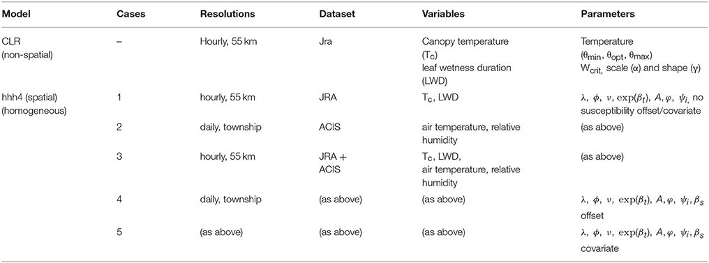
Table 1. A summary of input datasets, climate variable inputs, fixed parameters, data and model spatial, and temporal resolutions.

For the best-case, One-Step-Ahead forecasting was performed to approximate forecast error covariance. This was performed assuming a lead-time of a partial (1–4 weeks) and full season (1–11 weeks) time-window. The partial time-window could apply when forecasting disease within a growing season, while the longer time-window could apply when using data from a previous season in forecasting a future season. Four different statistical metrics or “scores” were evaluated in measuring the discrepancy between a model's predictive (i.e., “future” prediction is also termed a “forecast”) distribution, μ_P, and future observed value, y, namely: squared-error score (ses), logarithmic score (logs), Dawid-Sebastian (dss), and ranked-probability score (rps), given by,

$\begin{array}{l}\text{ses}:{(y-{\mu }_P)}^2\\ \text{logs}:{\frac{(y-{\mu }_P)}{{\sigma }_p^2}}^2+2\log {\sigma }_p\\ \text{dss}:{\frac{(y-{\mu }_P)}{2{\sigma }_p^2}}^2+2\log {\sigma }_p+\frac{1}{2}\log 2\pi \\ \text{rps}:E_{cdf,P}\left|Y-y\right|-\frac{1}{2}{E}_{cdf,P}\left|Y-Y\prime \right|& (9)\end{array}$

Y and Y′ are independent random variables associated with the distribution function p, y is a future “observed” or measured value, and μ_P and ${\sigma }_p^2$ are the mean and variance of the predictive (i.e., forecast) distribution, p. Both the location and spread of the forecast distribution are taken into account by the logs, dss and rps scores in judging how close the distribution is to the observed value. The rps score uses the predictive cumulative density function (cdf) and reduces to absolute error if p is a point-forecast rather than a distribution-forecast. It measures how well probability distribution-based forecasts match observed outcomes. These scores are summary measures of the predictive performance that allow for the joint assessment of calibration and sharpness are reviewed by Gneiting and Katzfuss (2014) and were computed using the surveillance R library package (Meyer S. et al., 2017). Lower scores indicate a model that has better predictive power, with mean scores used to identify a model with the best (i.e., minimal) forecast accuracy.

Results

Temperature response function parameters (θ_min, θ_opt, θ_max) for germination and appressorium formation (i.e., infection) were estimated using data, as (5.91, 15.41, 33.94) for germination, and (5.57, 15.57, 32.11) for infection (de Vallavieille-Pope et al., 1995). This optimal germination temperature range lies within the reported range (i.e., 16–18°C) of post-2000 Pst survival/occurrence at warmer temperatures (Chen, 2005; Xi et al., 2015) and previous reported estimates of (2.6,8.5,18) (Bregaglio et al., 2011). Critical wetness duration (W_crit) was set at 4 h, as a lower bound to the Pst reported range of 5–8 h (Bregaglio et al., 2011; Rolandson et al., 2015). The 4 h wetness duration estimate coincides with the timing of a rapid increase in infection for Pst, confirmed by experimental data under controlled conditions (de Vallavieille-Pope et al., 1995). This estimate also is close to observed mean wetness duration distribution peak for the ROI (Figure 4C). Risk distribution parameters (i.e., Weibull-distribution) of scale (α) and shape (γ) were estimated (α, γ), for germination as (13.36, 1.29) and for infection as (19.1, 2.14). The CLR (site-specific) model predictions (Figure 5) (scaled) are compared to observed Pst spore profile, collected at the Lethbridge site (Fairfield) during the 2015 wheat growing season [AIC = −749.47, root-mean-squared-error (RMSE) = 312.92].

FIGURE 5

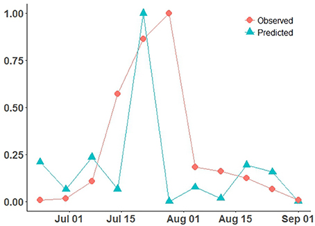
Figure 5. CLR model site-specific predicted Pst disease incidence (scaled 0–1), compared to the observed Pst airborne inoculum counts/profile collected at Lethbridge during the 2015 wheat growing season.

Best-fit estimates (and associated Standard Error) of the spatial model parameters are summarized for the 5 cases considered (Table 2). AIC values are provided under each case number in brackets. The predicted Pst spore population (for township region that contains the Lethbridge sampling site) through June-October for the 2015 growing season is shown against the observed Pst/airborne inoculum profile collected at the Lethbridge site (Figure 6A). Variability in these model predictions (case 3) for neighboring regions surrounding the Lethbridge township is shown for this particular season (2015) and subregion, to be strongly endemic, with low autoregressive and transmission contributions from neighboring regions (Figure 6B). Estimates forecast scores obtained from one-step-ahead model forecasting are summarized in b. The two different lead-times assume: (i) only Pst population information for the first few weeks (i.e., weeks 1–4 occurring before the main infection peak) is available, and (ii) full data for the entire season is available.

TABLE 2

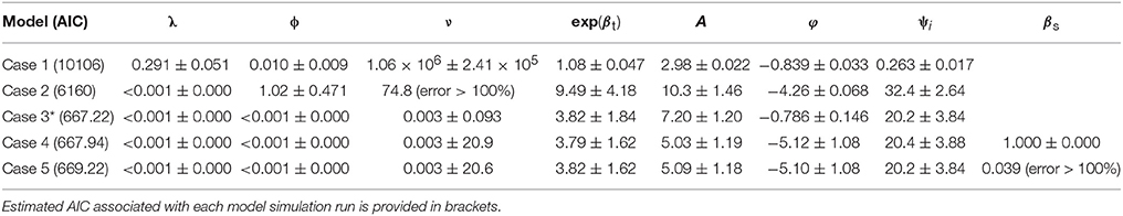
Table 2. Best-fit estimates of the hhh4 homogeneous model parameters (Equations 5, 6) and associated Standard Errors (SE) for endemic, ν, and epidemic [i.e., autoregressive, λ = exp(α(^λ)) , and spatio-temporal, ϕ = exp(α(^ϕ))] contributions are shown for each of the cases considered: case 1—JRA reanalysis only (∼55 km), case 2—ACIS climate only (∼10 km), and case 3—multiscale with both JRA and ACIS, and two susceptibility corrections of the best-fitting homogeneous model i.e., case 3 (indicated by *) (case 4—offset type, case 5—covariate type).

FIGURE 6

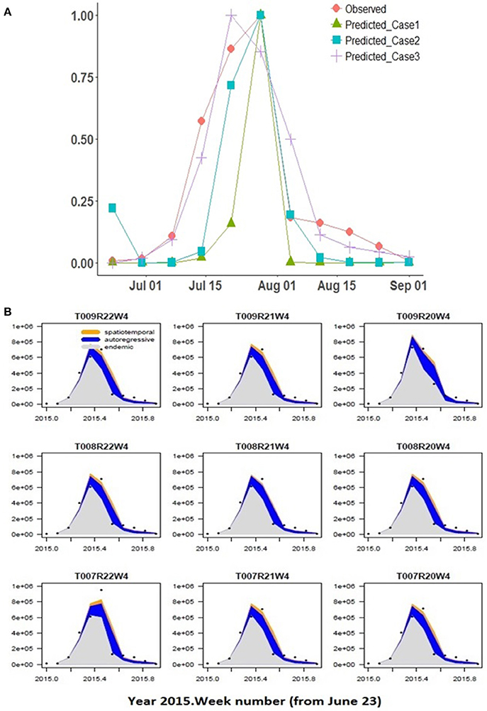
Figure 6. (A) Spatial model predictions of the hhh4 model for cases 1–3 with different climate input data are shown compared to observed at the Lethbridge collection site, (B) Predicted Pst disease incidence (scaled 0–1) within the Lethbridge township (TW008R21W4) and its neighboring townships for the best-fitting model (case 3) vs. number of weeks. Variability in the endemic, autoregressive, and spatio-temporal contributions are shown driven by climate variability across the regions.

Discussion

The site-specific model (CLR) with the coarser JRA reanalysis input was able to reproduce the general shape of the observed Pst detection (2015 at Lethbridge) based on the assumptions of critical thresholds of wetness and temperature-response, and independent, Weibull-distributed germination/infection processes (Figure 5). The model predicts the rate of infection (slope of mid-season peak) well, but predicts a narrower peak width (timing of main infection peak rise and fall) and predicts peak infection a week earlier than it occurred. Predictions of the model are more variable during the early- and late-season, which is attributed to higher variability in the weather conditions (i.e., fluctuations in canopy wetness and temperature shown in Figures 4B,C). Using the same coarse JRA climate input data, the spatial hhh4 model with spatial transmission assumptions (case 1), while not the best fit obtained to the observed infection curve, like the CLR site-specific model, does also predict a narrow peak. However, the hhh4 model predictions are less variable in early/late season and it predicts peak infection time correctly (Figure 6). This indicates that assumptions on how Pst immigrates, overwinters and moves between subregions, are important for accurately determining both infection variability in early/late season as well as the timing of peak infection. Changing the spatial resolution of climate input data (i.e., from JRA regional-scale in case 1 to finer ACIS township-scale in case 2), improved the prediction of width of the infection peak, which is especially crucial, as it is at this time that disease dynamics can switch from an endemic, to an epidemic disease occurrence pattern.

Finer scale climate input improved the ability of the spatial hhh4 model to predict Pst disease dynamics (case 2 vs. case 1) (Figure 6). The best-performing model (hhh4 case 3 with lowest AIC) (Table 2) had the strongest endemic contribution (initial deposition followed by weak transmission of Pst through the growing season, measured at the Lethbridge site). Comparing AIC values for the various cases of the hhh4 model (see Table 2) in terms of relative gain in accuracy [i.e., (|AIC_old-AIC_new|/|AIC_old|) x100%, where AIC_old denotes the model with the higher AIC, and AIC_new the improved model with the lower AIC] provides quantification of the various improvements (spatial and temporal resolution, and inclusion of a susceptibility correction as an offset or covariate). Changing spatial resolution (55 km to township/10 km) and temporal resolution (hourly to daily) led to a relative improvement in accuracy (relative reduction in AIC) of 64% (case 2 vs. case 1). A further relative accuracy gain of 89% was achieved by combining information at different spatial and temporal scale (i.e., hourly and daily, 55 km and township/10 km) (multi-scale case 3 vs. case 2). Correcting for susceptibility as an offset led to a relative accuracy gain of < 1% , and no change as a covariate, but these quantified changes are more unreliable due to associated increases in the standard error of model parameters. Overall all cases, the best case (Case 3) was identified or defined as the model case that had the lowest AIC value or highest forecast accuracy) used multi-scale JRA and ACIS data and assumed no correction for susceptibility. The worst-case (Case 1) was identified as the model case that had the highest AIC value or lowest forecast accuracy using only JRA data and assuming no correction for sustainability. Case 3 not only obtained the lowest AIC, but also produced more accurate estimates of the endemic parameter (smaller standard error). This case explains the data the best (with the lowest AIC) as having weak epidemic components, but strong endemic component, even though the standard error in some model parameters relative to their estimated value increased. Case 3, with the lowest AIC value (best case model), when compared to the highest AIC value (Case 1 worst case model) has a relative overall gain of 93.4% in model accuracy.

The small accuracy improvement offered by a susceptibility correction could be, in part, due to the homogeneous modeling assumptions. Accounting for susceptibility in the best-fit model (case 3), reduced model accuracy only slightly. More observed airborne inoculum sampling data would considerably reduce the high standard error (SE) of the intercept and susceptibility coefficient parameters $({\alpha }^{(\nu )},{\beta }_s)$. Considering susceptibility as an endemic offset, rather than an epidemic autoregressive/covariate effect, produced a model with slightly higher accuracy. This was largely determined, however, by weather variability. Accounting for susceptibility increased the uncertainty in the endemic parameter considerably, pointing to the need for heterogeneous assumptions, alongside a larger data from Pst airborne surveillance in the region to reduce it. This also indicates that the susceptibility parameter is a useful metric for gauging disease risk and determining where to optimally monitor for Pst across the entire ROI. Additional susceptibility effects could be considered if heterogeneous assumptions were considered in the hhh4 model, whereby a multi-variate, “susceptibility function” could be defined (i.e., that further modifies Equations 7, 8). This function could integrate specific-cultivar attributes and/or fungicide control/spray data, and potential canopy changes due to disease detected from available vegetation index satellite data (Davidson, 2015; Devadas et al., 2015). More complex forms of the hhh4 spatial model with spatial-interaction assumptions, heterogeneity driven by long-range transmission, and higher-order neighbors/transmission across sub-regions (power law or second-order model) could be considered. Also, independent random effects uncertainty could be included that typically results from unobserved heterogeneity due to under-reporting of disease occurrence. The hhh3 case 3 model (relying on multi-resolution climate data and spatial dependence assumptions) had reasonable ranges of the predictive assessment scores (Table 3). Based on a test period of 4 weeks (i.e., in June-July in advance of peak infection) the best-fit model is able to forecast with 50% accuracy (using the full window of 11 weeks as a benchmark). This forecast accuracy was achieved using airborne inoculum data for a single site and season, alongside disease, environment and susceptibility assumptions. A larger dataset of Pst infection data would enable a more reliable determination of the forecast accuracy of this model and reliable attribution of forecast error to environmental (i.e., climate/weather) variability, and/or host-pathogen disease dynamics.

TABLE 3

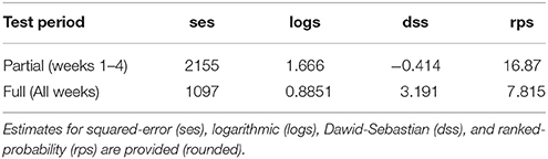
Table 3. Performance of model-based forecasting (4 scores) for Pst disease (i.e., disease risk) within southern Alberta in 2015 for a partial and complete season lead-time, using the best training case (case 3) of the hhh4 model.

In summary, the integrated framework proposed offers a feasible way to combine diverse datasets and models with a wide range of assumptions to explain variability and uncertainty in observed disease incidence patterns and to forecast risk. Current findings show that the more complex, stochastic model (hhh4) using weather station network data with susceptibility correction provides sufficient accuracy and reliability. Machine-learning may further improve model-based disease risk forecasting under highly unpredictable weather or management regimes (Liao and Ji, 2009; Wen et al., 2017). Testing the feasibility of this framework and modeling approach relied on limited airborne inoculum data for Pst (i.e., available and high-quality controlled data from the recent 2015 season at Lethbridge) and homogeneous assumptions. Nonetheless, this is the first time such data has been collected for Pst in this region of interest. Current findings are supported by the integration of knowledge, parameter estimates, multiple evidence sources (i.e., published empirical data on Pst, included latest available, quality-controlled climate, satellite and airborne inoculum).

An expanded evaluation of model-based forecast accuracy will require a large, seasonal airborne surveillance program and heterogeneous assumptions. Heterogeneous assumptions would help to fine-scale incidence and risk variability based on measured changes in endemic-epidemic transition time, maximum infection potential, infection peak timing, and width between regions. The most accurate, efficient, and cost-effective airborne surveillance monitoring plan may be a multi-resolution sampling design that could sample disease across the full extent of a large ROI at a coarser resolution, while sampling denser, at a finer resolution within known disease hotspots. This is supported by the current findings; the spatial model (case 1) using coarser climate input predicted an underlying pattern of Pst occurrence that is under-dispersed (ψ_i < 1), while cases 2 and 3 indicated it is over-dispersed (ψ_i>1)_. Given case 3 fit the observed data better, a more clumped, concentrated pattern is inferred for Pst based within the 2015 growing season. Hotspots could be identified as townships or subregions where a disease overwinters/oversummers across a sufficient number of sampling seasons, or higher risk clusters of townships within which Pst disease is first or early-detected. Susceptibility offsets and covariation provides an important spatial-based sustainability metric for gauging subregions where disease risk may be highest and where to more intensively sample (Kouadio and Newlands, 2015). Extensions of the spatial model could also include viability of inoculum (i.e., variability in the different isolates that are present into a “natural” inoculum). In laboratory studies, often a single isolate is used. Field studies can involve both a single or composite inoculum; when a composite, one can consider a number of different characterized isolates or assume that a field isolate that was present in a previous growing season has been amplified (multiplied) and is re-inoculating. Also, in further expanded modeling and with the availability of spore data for 2016-2018, the models could be run for the 2019 growing season to predict disease risk, using hourly/daily climate data across all past 4 years where spore data was being collected (i.e., 2015-2018). The 2016-18 time period could be then used to provide training/calibration data for the models, and uncertainty in the model fixed parameters and current season disease risk could be compared to an uncertainty range estimated using all past climate information. This would also provide a historical prediction range to compare against a current-season prediction range. A multi-scale airborne surveillance design that provides data to support operational model-based disease risk forecasting, may, in the future, enable more reliable, timely and cost-effective decisions in sustaining crop yields against multiple disease threats. Developing an integrated understanding of disease risks, impacts, consequences (whether anticipated or unanticipated), alongside decision trade-offs, could provide crucial, cornerstone insights to controlling crop disease, and increasing crop yields sustainably.

Author Contributions

The author confirms being the sole contributor of this work and approved it for publication.

Conflict of Interest Statement

The author declares that the research was conducted in the absence of any commercial or financial relationships that could be construed as a potential conflict of interest.

Acknowledgments

NN was supported by Growing Forward II Federal Research Program (Agriculture and Agri-Food Canada, AAFC) funding (Project No. J-000179.001.02). My thanks to AAFC colleagues: Mr. Weixun Lu (AAFC-Summerland) for providing R language coding assistance, Mr. Kieran Forge for help in preparing disease incidence maps in ArcGIS (ESRI Inc., Ver. 10.4). I thank Dr. André Laroche (AAFC-Lethbridge) for providing the 2015 season wheat stripe rust inoculum data and comments on an earlier draft of this manuscript. I thank Dr. T. A. Porcelli for providing helpful feedback and editorial assistance. I thank two reviewers for feedback that helped to improve this manuscript.

Footnotes

1. ^Alberta Climate Information Service (ACIS): https://agriculture.alberta.ca/acis/.

2. ^Water weight to water column: 1 kg m⁻² = 1 mm = 0.001 m, T(°C) = T(K) − 273.15.

References

Ali, S., Rodriguez-Algaba, J., Thach, T., Sørensen, C. K., Hansen, J. G., Lassen, P., et al. (2017). Yellow rust epidemics worldwide were caused by pathogen races from divergent genetic lineages. Front. Plant Sci. 8:1057. doi: 10.3389/fpls.2017.01057

PubMed Abstract | CrossRef Full Text | Google Scholar

Anonymous (2018). Government of Western Australia (Department of Primary Industries and Regional Development). Available online at: https://www.agric.wa.gov.au/grains-research-development/managing-stripe-rust-and-leaf-rust-wheat-western-australia (Accessed May 5, 2018).

Araujo, G. T., Amundsen, E., Gaudet, D., Selinger, B. L., and Laroche, A. (2016). “Incidence of important fungal wheat pathogens in western Canada,” in 50th Annual Prairie University Biology Symposium(Lethbridge, AB: University of Lethbridge).

Audsley, E., Milne, A., and Paveley, N. (2005). A foliar disease model for use in wheat disease management decision support systems. Ann. Appl. Biol. 147, 161–172. doi: 10.1111/j.1744-7348.2005.00023.x

CrossRef Full Text | Google Scholar

Bebber, D. P., Castillo, A. D., and Gurr, S. J. (2016). Modelling coffee leaf rust in Columbia with climate reanalysis data. Philos. Trans. R. Soc. B 371:20150458. doi: 10.1098/rstb.2015.0458

CrossRef Full Text | Google Scholar

Braithwaite, M., Cromey, M. G., Saville, D. J., and Cookson, T. (1998) “Effects of fungicide rates timing on control of stripe rust in wheat Arable Crops,” in Proc. 51^st. N.Z. Plant Protection Conf, 66–70. Available online at: https://www.researchgate.net/publication/266356024

Bregaglio, S., Cappelli, G., and Donatelli, M. (2012). Evaluating the suitability of a generic fungal infection model for pest risk assessment studies. Ecol. Modell. 247, 58–63. doi: 10.1016/j.ecolmodel.2012.08.004

CrossRef Full Text | Google Scholar

Bregaglio, S., Donatelli, M., Confalonieri, R., Actuis, M., and Orlandini, S. (2011). Multi-metric evaluation of leaf wetness models for large-area application of plant disease models. Agric. For. Meteorol. 151, 1163–1172. doi: 10.1016/j.agrformet.2011.04.003

CrossRef Full Text | Google Scholar

Bryant, R. R., McGrann, G. R. D., Mitchell, A. R., Schoonbeek, H.-J., Boyd, L. A., Uauy, C., et al. (2014). A change in temperature modulates defence to yellow (stripe) rust in wheat line UC1041 independently of resistance gene Yr36. BMC Plant Biol. 14:10. doi: 10.1186/1471-2229-14-10

PubMed Abstract | CrossRef Full Text | Google Scholar

Carisse, O., Bacon, R., and Lefebvre, A. (2009). Grape powdery mildew (Erysiphe necator) risk assessment based on airborne conidium concentration. Crop Prot. 28, 1035–1044. doi: 10.1016/j.cropro.2009.06.002

CrossRef Full Text | Google Scholar

Chakraborty, S., and Newton, A. C. (2011). Climate change, plant diseases and food security: an overview. Plant Pathol. 60, 2–14. doi: 10.1111/j.1365-3059.2010.02411.x

CrossRef Full Text | Google Scholar

Chamecki, M., Dufault, D. S., and Isard, S. A. (2012). Atmospheric dispersion of wheat rust spores: A new theoretical framework to interpret field data and estimate downwind dispersion. J. Appl. Meteor. Climatol. 51, 672–685. doi: 10.1175/JAMC-D-11-0172.1

CrossRef Full Text | Google Scholar

Chen, W., Wellings, C., Chen, X., Kang, Z., and Liu, T. (2014). Pathogen profile: wheat stripe (yellow) rust caused by Puccinia striiformis f. sp. tritici. Mol. Plant Pathol. 15, 433–446. doi: 10.1111/mpp.12116

CrossRef Full Text | Google Scholar

Chen, X. M. (2005). Review: epidemiology and control of stripe rust (Puccinia striiformis f. sp. tritici) on wheat. Can. J. Plant Pathol. 27, 314–337. doi: 10.1080/07060660509507230

CrossRef Full Text | Google Scholar

Chen, X. M. (2007). Challenges and solutions for stripe rust control in the United States. Austr. J. Agric. Res. 58, 648–655. doi: 10.1071/AR07045

CrossRef Full Text | Google Scholar

Chen, X. M. (2010). Race Summary of Puccinia striiformis f. sp. tritici (Wheat Stripe Rust) and P. striiformis f. sp. hordei (Barley Stripe Rust) in the United States in 2010. Available online at: http://striperust.wsu.edu/races/data/ (Accessed June 15, 2018).

Conner, R. L., Thomas, J. B., and Kuzyk, A. D. (1988). Overwintering of stripe rust in southern Alberta. Can. Plant Dis. Surv. 68, 153–155.

Google Scholar

Contreras-Medina, L. M., Torres-Pacheco, I., Guevara-González, R. G., Romero-Troncoso, R. J., Terol-Villalobos, I. R., and Osornio-Rios, R. A. (2009). Mathematical modeling tendencies in plant pathology. Afr. J. Biotechnol. 8, 7399–7408. Available online at: https://www.ajol.info/index.php/ajb/article/view/77754/68176

Google Scholar

Davidson, A. (2015). An Operational Canadian Ag-Land Monitoring System (CALMS): Near-Real-Time Agricultural Assessment From Space. Agriculture and Agri-Food Canada, 60. Available online at: http://www.agr.gc.ca/atlas/supportdocument_documentdesupport/aafcModisNdvi/en/Background_to_the_MODIS_NDVI_Composites.pdf (Accessed Nov 15, 2017).

de Vallavieille-Pope, C., Huber, L., Leconte, M., and Goyeau, H. (1995). Comparative effects of temperature and interrupted wet periods on germination, penetration, and infection of Puccinia recondita f. sp. tritici and P. striiformis on wheat seedlings. Ecol. Epidemiol. 85, 409–415.

Google Scholar

Dennis, J. I. (1987). Temperature and wet-period conditions for infection by Puccinia striiformis f.sp tritici race 104E137A+. Trans. Br. Mycol. Soc. 88, 119–121.

Google Scholar

Devadas, R., Lamb, D. W., Blackhouse, D., and Simpfendorfer, S. (2015). Sequential application of hyperspectral indices for delineation of stripe rust infection and nitrogen deficiency in wheat. Precision Agric. 16, 477–491. doi: 10.1007/s11119-015-9390-0

CrossRef Full Text | Google Scholar

El Jarroudi, M., Kouadio, A., Bock, C. H., El Jarroudi, M., Junk, J., Pasquali, M., et al. (2017). A threshold-based weather model for predicting stripe rust infection in winter wheat. Plant Dis. 101, 693–703. doi: 10.1094/PDIS-12-16-1766-RE

CrossRef Full Text | Google Scholar

Food Agriculture Organization of the United Nations (FAO) (2018). World Food Situation: FAO Cereal Supply and Demand Brief . Available online at: http://www.fao.org/worldfoodsituation/csdb/en/ (Accessed, May 11, 2018).

Gneiting, T., and Katzfuss, M. (2014). Probabilistic forecasting. Ann. Rev. Stat. Appl. 1, 125–151. doi: 10.1146/annurev-statistics-062713-085831

CrossRef Full Text | Google Scholar

Haran, M., Bhat, K. S., Molineros, J., and De Wolf, E. (2010). Estimating the risk of a crop epidemic from coincident spatio-temporal processes. J. Agric. Biol. Environ. Stat. 15, 158–175. doi: 10.1007/s13253-009-0015-9

CrossRef Full Text | Google Scholar

Held, L., and Paul, M. (2012). Modeling Seasonality in space-time infectious disease surveillance data. Biometr. J. 54, 824–843. doi: 10.1002/bimj.201200037

PubMed Abstract | CrossRef Full Text | Google Scholar

Held, L., Höhle, M., and Hofmann, M. (2004). “A statistical framework for the analysis of multivariate infections disease surveillance data,” Paper 402 Ludwig-Maximilians-Universität Munchen, Insitute Fur Statistik Sonderforschungsbereich 386. Available online at: http://epub.ub.uni-muenchen.de/ (Accessed Nov 15, 2017).

Höhle, M., Meyer, S., Paul, M., Held, L., Burkom, H., Correa, T., et al. (2017). Temporal and Spatio-Temporal Modeling and Monitoring of Epidemic Phenomena. Surveillance R package version 1.15.0. Available online at: http://surveillance.r-forge.r-project.org/ (Accessed Nov. 15, 2017).

Hovmøller, M. S. (2001). Disease severity and pathotype dynamics of Puccinia striiformis f.sp. tritici in Denmark. Plant Pathol. 50, 181–189. doi: 10.1046/j.1365-3059.2001.00525.x

CrossRef Full Text | Google Scholar

Isard, S. A., Barnes, C. W., Hambleton, S., Ariatti, A., Russo, J. M., Tenuta, A., et al. (2011). Predicting soybean rust incursions into the North American continental interior using crop monitoring, spore trapping, and aerobiological modeling. Plant Dis. 95, 1346–1357. doi: 10.1094/PDIS-01-11-0034

CrossRef Full Text | Google Scholar

Juroszek, P., and von Tiedemann, A. (2013). Climate change and potential future risks through wheat diseases: a review. Eur. J. Plant Pathol. 136, 21–33. doi: 10.1007/s10658-012-0144-9

CrossRef Full Text | Google Scholar

Kobayashi, S., Ota, Y., Harada, Y., Ebita, A., Moriya, M., Onoda, H., et al. (2015). The JRA-55 reanalysis: general specifications and basic characteristics. J. Meteorol. Soc. Jpn. Ser. II. 93, 5–48. doi: 10.2151/jmsj.2015-001

CrossRef Full Text | Google Scholar

Kouadio, L., and Newlands, N. K. (2015). Building capacity for spatial-based sustainability metrics in agriculture. Decis. Anal. 2:2. doi: 10.1186/s40165-015-0011-9

CrossRef Full Text | Google Scholar

Kuang, W., Liu, W., Ma, Z., and Wang, H. (2013). “Development of a web-based prediction system for wheat stripe rust,” in 6th Computer and Computing Technologies in Agriculture (CCTA), Oct 2012, Zhangjiajie, China. Springer, IFIP Advances in Information and Communication Technology, AICT-392 (Part I), Computer and Computing Technologies in Agriculture VI, 324–335. Available online at: https://hal.inria.fr/hal-01348115 (Accessed Nov 15, 2017).

Google Scholar

Laroche, A., Araujo, G. T., Lu, W., Amundsen, E., Newlands, N. K., Aboukhaddour, R., et al. (2018). “Aerobiological surveillance of wheat pathogens,” in Conference Proceedings of Agronomy Update 2018 (Red Deer, AB), 52.

Lei, Y., Wang, M., Wan, A., Xia, C., See, D. R., Zhang, M., and Chen, X. (2017). Virulence and molecular characterization of experimental isolates of the stripe rust pathogen (Puccinia striiformis) indicate stomatic recombination. Phytopathology 107, 329–344. doi: 10.1094/PHYTO-07-16-0261-R

PubMed Abstract | CrossRef Full Text | Google Scholar

Liao, W., and Ji, Q. (2009). Learning Bayesian network parameters under incomplete data with domain knowledge. Pattern Recognit. 42, 3036–3056. doi: 10.1016/j.patcog.2009.04.006

CrossRef Full Text | Google Scholar

Mahlein, A.-K. (2016). Plant disease detection by imaging sensors – parallels and specific demands for precision agriculture and plant phenotyping. Plant Dis. 100, 241–251. doi: 10.1094/PDIS-03-15-0340-FE

CrossRef Full Text | Google Scholar

Meyer, M., Cox, J. A., Hitchings, M. D. T., Burgin, L., Hort, M. C., Hodson, D. P., et al. (2017). Quantifying airborne dispersal routes of pathogens over continents to safeguard global wheat supply. Nat. Plants Lett. 3, 780–796. doi: 10.1038/s41477-017-0017-5

PubMed Abstract | CrossRef Full Text | Google Scholar

Meyer, S., Held, L., and Höhle, M. (2017). Spatio-temporal analysis of epidemic phenomena using the R Package surveillance. J. Stat. Soft. 77, 1–55. doi: 10.18637/jss.v077.i11

CrossRef Full Text | Google Scholar

Minchinton, E. J., Auer, D. P. F., Thomson, F. M., Trapnell, L. N., Galea, V., Faggian, R., et al. (2013). Evaluation of the efficacy and economics of irrigation management, plant resistance and Brassica ${}_{\text{spot}}^{(\text{TM})}$ models for management of white blister on Brassica crops. Austral. Plant Pathol. 42, 169–178. doi: 10.1007/s13313-012-0181-z

CrossRef Full Text | Google Scholar

Newberry, F., Qi, A., and Fitt, B. D. L. (2016). Modelling impacts of climate change on arable crop diseases: progress, challenges and applications. Curr. Opin. Plant Biol. 32, 101–109. doi: 10.1016/j.pbi.2016.07.002

CrossRef Full Text | Google Scholar

Newlands, N. K. (2016). Future Sustainable Ecosystems: Complexity, Risk, Uncertainty. Boca Raton, FL: Taylor & Francis (Chapman & Hall/CRC Applied Environmental Statistics Series), 418.

Google Scholar

Nicolopoulou-Stamati, P., Maipas, S., Kotampasi, C., Stamatis, P., and Hens, L. (2016). Chemical pesticides and human health: the urgent need for a new concept in agriculture. Front. Public Health 4:148. doi: 10.3389/fpubh.2016.00148

PubMed Abstract | CrossRef Full Text | Google Scholar

Nopsa, J. F. H., and Pfender, W. F. (2014). A latent period duration model for wheat stem rust. Plant Dis. 98, 1358–1363. doi: 10.1094/PDIS-11-13-1128-RE

CrossRef Full Text | Google Scholar

Ojiambo, P. S., Yuen, J., van den Bosch, F., and Madden, L. V. (2017). Epidemiology: past, present and future impacts on understanding disease dynamics and improving plant disease management – A summary of focus issue articles. Phytopathology 107, 1092–1094. doi: 10.1094/PHYTO-07-17-0248-FI

PubMed Abstract | CrossRef Full Text | Google Scholar

Parsons, D. J., and Te Beest, D. (2004). Optimising fungicide applications on winter wheat using genetic algorithms. Biosyst. Eng. 88, 401–410. doi: 10.1016/j.biosystemseng.2004.04.012

CrossRef Full Text | Google Scholar

Paul, M., and Meyer, S. (2016). hhh4: An Endemic-Epidemic Modelling Framework for Infectious Disease Counts. Available online at: https://cran.r-project.org/web/packages/surveillance/vignettes/hhh4.pdf (Accessed Nov. 15, 2017).

Peshin, R., Bandral, R. S., Zhang, W., Wilson, L., and Dhawan, A. K. (2009). “Integrated pest management: a global overview of history, programs and adoption,” in Integrated Pest Management: Innovation-Development Process, eds R. Peshin and A. K. Dhawan (Dordrecht: Springer), 1–46.

Google Scholar

Phillips, A. J., and Newlands, N. K. (2011). Spatial and temporal variability of soil freeze-thaw cycling across southern Alberta Canada. Agric. Sci. 2, 392–405. doi: 10.4236/as.2011.23051

CrossRef Full Text | Google Scholar

Pretty, J., and Bharucha, Z. P. (2015). Integrated pest management for sustainable intensification pf agriculture in Asia and Africa. Insects 6, 152–182. doi: 10.3390/insects6010152

PubMed Abstract | CrossRef Full Text | Google Scholar

R Core Team (2017). R: A Language and Environment for Statistical Computing. Vienna: R Foundation for Statistical Computing. Available online at: http://www.R-project.org/ (Accessed Nov 15, 2017).

Riley, S., Earnes, K., Isham, V., Mollison, D., and Trapman, P. (2015). Five challenges for spatial epidemic models. Epidemics 10, 68–71. doi: 10.1016/j.epidem.2014.07.001

PubMed Abstract | CrossRef Full Text | Google Scholar

Rolandson, T., Gleason, M., Sentalhas, P., Gellespie, T., Thomas, C., and Hornbuckle, B. (2015). Reconsidering leaf wetness duration determination for plant disease management. Plant Dis. 99, 310–319. doi: 10.1094/PDIS-05-14-0529-FE

CrossRef Full Text | Google Scholar

Sadyś, M., Skjøth, C. A., and Kennedy, R. (2016). Forecasting methodologies for Ganoderma spore concentration using combined statistical approaches and model evaluations. Int. J. Biometeor. 60, 489–498. doi: 10.1007/s00484-015-1045-3

PubMed Abstract | CrossRef Full Text | Google Scholar

Savage, D., and Renton, M. (2014). Requirements, design and implementation of a general model of biological invasion. Ecol. Modell. 272, 394–409.

Google Scholar

Schwessinger, B. (2017). Fundamental wheat stripe rust research in the 21^st Century. New Pathol. 213, 1625–1631. doi: 10.1111/nph.14159

PubMed Abstract | CrossRef Full Text | Google Scholar

Sharma-Poudyal, D. (2012). Prediction of Disease Damage, Determination of Pathogen Survival Regions, and Characterization of International Collections of Wheat Stripe Rust. Ph.D. Thesis, Washington State University. Available online at: https://research.wsulibs.wsu.edu/xmlui/bitstream/handle/2376/4061/SharmaPoudyal_wsu_0251E_10339.pdf?sequence=1 (Accessed Nov. 15, 2017).

Sharma-Poudyal, D., Chen, X., and Rupp, R. A. (2014). Potential oversummering and overwintering regions for the wheat stripe rust pathogen in the contiguous United States. Int. J. Biometeorol. 58, 987–997. doi: 10.1007/s00484-013-0683-6

PubMed Abstract | CrossRef Full Text | Google Scholar

Tran, V. A., and Kutcher, H. R. (2015). “Temperature effects on the aggressiveness of Puccinia striiformis f. sp. tritici, stripe rust of wheat,” Soil and Crops Workshop, University of Saskatchewan, 6. Available online at: http://www.usask.ca/soilsncrops/conference-proceedings/index.php (Accessed Nov. 15, 2017).

Google Scholar

Wang, M., and Chen, X. (2017). “Stripe Rust Resistance,” (Chapter 5) in Stripe Rust, eds X. M.Chen and J. Kang (Dordrecht: Science+Business Media B.V.), 353–558.

Wen, L., Bowen, C. R., and Hartman, G. L. (2017). Prediction of short-distance aerial movement of Phakopsora pachyrhizi urediniospores using machine learning. Phytopathology 107, 1187–1198. doi: 10.1094/PHYTO-04-17-0138-FI

PubMed Abstract | CrossRef Full Text | Google Scholar

West, J., and Kimber, R. (2015). Innovations in air sampling to detect plant pathogens. Ann. Appl. Biol. 166, 4–17. doi: 10.1111/aab.12191

PubMed Abstract | CrossRef Full Text

World Bank Group (2017). Commodity Market Outlook. Washington, DC: World Bank.

Xi, K., Kumar, K., Holtz, M. D., Turkington, T. K., and Chapman, B. (2015). Understanding the development and management of stripe rust in central Alberta. Can. J.Plant Pathol. 37, 21–39. doi: 10.1080/07060661.2014.981215

CrossRef Full Text | Google Scholar

Yan, W., and Hunt, L. A. (1999). An equation for modelling the temperature response of plants using only the cardinal temperatures. Ann. Bot. 84, 607–614.

Google Scholar