Spatial Variability and Hotspots of Methane Concentrations in a Large Temperate River

1 Introduction

Awareness regarding the significant contributions of inland waters, such as lakes, reservoirs, or rivers, to the global CH₄ budget (103 Tg CH₄ year⁻¹) has been increasing (Rosentreter et al., 2021); however, relatively few studies have investigated CH₄ dynamics in flowing waters (Bastviken et al., 2011). Streams and rivers have garnered much attention as the sources of atmospheric CH₄ (Stanley et al., 2016). Regardless of being well-aerated, lotic waters are typically oversaturated with CH₄ compared to water in equilibrium with atmospheric CH₄, resulting in significant diffusive emissions to the atmosphere (Stanley et al., 2016). However, the precise quantification of these CH₄ emissions is challenging because of large spatiotemporal heterogeneities. The magnitude of these diffusive emissions depends on the water turbulence, physical gas transfer coefficient, and CH₄ partial pressure difference between water and the atmosphere (Donelan et al., 2002).

Dissolved CH₄ concentrations are rather variable and depend on the balance between the input of CH₄ to water and its loss. While outgassing to the atmosphere is the most important CH₄ loss process, microbial CH₄ consumption in the water is relatively slow (Matoušů et al., 2019). The main sources of CH₄ are in-stream production in anoxic sediments and import from riparian areas (Rasilo et al., 2017). The hydrologic linkage to suitable habitats such as inundated floodplains and wetlands delivers CH₄ to the river channel (Stanley et al., 2016). Recently, possible phytoplankton-mediated CH₄ production under oxic conditions has been discussed (Tang et al., 2016).

However, localized input of CH₄ to streams is not simple to detect, because outgassing is a rapid process, resulting in a short residence time of CH₄ in stream water (in River Elbe less than a day). Furthermore, the low solubility of CH₄ in the water coupled with its rapid water–atmosphere exchange can lead to pronounced heterogeneities in CH₄ concentrations along the river gradient. Any CH₄ input to a stream is lost to the atmosphere within a short flow distance, resulting in the local control of CH₄ concentrations in streams (Stanley et al., 2016).

Conventional assessments of spatial heterogeneity in streams rely on discrete sampling, restricting the amount of possible data and spatial resolution. In a previous study also along the Elbe, large-scale patterns and hotspots of elevated CH₄ concentrations have been revealed (Matoušů et al., 2019). In particular, harbors, dammed river sections, and tributary inflows are the well-known CH₄ emission hotspots (Maeck et al., 2013), which are often neglected in conventional sampling schemes. Therefore, upscaling based on such conventional datasets entails a high degree of uncertainty, because the employed approaches may overlook local hotspots and the spatial extent of such hotspots may be poorly defined.

A number of approaches can be used to quantify CH₄ concentrations and detect CH₄ emission hotspots. To measure dissolved CH₄ at a high spatial resolution, several degassing systems coupled with cavity ring-down spectroscopy have been used (Gonzalez-Valencia et al., 2014). Alternatively, in-situ CH₄ sensors can be used to map CH₄ (Canning et al., 2021). Moreover, CH₄ point emission sources can be identified based on atmospheric measurements using a hyperspectral camera (Gålfalk et al., 2016) or mobile gas analyzer (Karion et al., 2013). Atmospheric CH₄ measurements from autonomous boats have been used to map CH₄ emissions from freshwaters (Dunbabin and Grinham 2017).

To this end, we scanned a 584 km longitudinal transect along the Elbe—Germany’s third largest river—including the mouth of several tributaries. We simultaneously and continuously measured dissolved and atmospheric CH₄ concentrations using a degassing system connected to a greenhouse gas analyzer. In addition, we measured basic hydrographic parameters. This allowed a novel and high spatial resolution of about 4000 data points. The present study aimed to quantify CH₄ concentrations in and identify CH₄ hotspots along the river channel. By analyzing a quasi-continuous dataset of CH₄ concentrations we tried to identify and characterize possible sources of CH₄, which is hardly possible with single water samples along the river. Finally, by monitoring the CH₄ mixing ratio in the atmosphere in parallel, we explored the potential effects of fluctuating atmospheric CH₄ concentrations on the calculated CH₄ emissions, the possibility of detecting hotspots based on atmospheric measurements and thus to improve the estimation of the diffusive CH₄ flux from the Elbe.

2 Materials and Methods

2.1 Study Area: German Elbe and its Tributaries

River Elbe is 1,094-km-long, flowing from the Czech Republic to the North Sea. The catchment area spans 148,268 km², and the mean annual discharge is 861 m³ s⁻¹ at the mouth. The present study covers the German part of the river between the Czech border (Elbe km-0) and Geesthacht weir (Elbe km-586). Discharge at the gauge Magdeburg at the time of the study was 241 m³ s⁻¹, which is close to the average low value (231 m³ s⁻¹) and 44% of the annual mean (554 m³ s⁻¹). Elbe flows through several land use types, including highly urbanized zones, agricultural regions, and near-natural areas. Major tributaries are the rivers Schwarze Elster, Mulde, Saale, and Havel. Here, we primarily focused on the effects of Havel on dissolved CH₄ in the Elbe. Additional information on the tributaries is provided in the Supplementary Material.

2.2 Vessel Cruise and Water Sampling

Sampling was performed using the research vessel Albis, which is 15-m-long and has a draft of only 45 cm. We used the Lagrangian approach in which sampling was performed according to the travel time of the river water. The cruise started on 4 August 2020, in Schmilka (Elbe km-4) and was completed on 12 August 2020, in Geesthacht (Elbe km-584, Figure 1). The positions recorded by GPS (longitude and latitude) were converted to “Elbe kilometer” together with information on the lateral distance to the middle of the navigation channel (https://atlas.wsv.bund.de/bwastr-locator/client/).

FIGURE 1

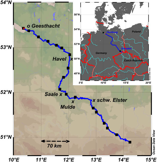
FIGURE 1. Map of the studied part of German. The inlet shows the location of the Elbe (blue) within Europe (red border lines) and other rivers (light blue).

At 23 stations, a transect across the river channel was sampled (left-hand shore, middle, and right-hand shore, Figure 1). Each time the anchor was set, sampling was performed for approximately 10 min. In addition, river water was pumped continuously from the vessel bottom to a pool, which provided water to all continuous measurement devices.

For CH₄ analyses, 30 ml water samples were collected with a horizontal water sampler (Hydro-Bios, Germany) and 60 ml plastic syringes. A headspace of 30 ml ambient air was created, and the syringes were vigorously shaken for 2 min. The equilibrated headspace was transferred to evacuated Exetainer vials (Labco, United Kingdom), and the equilibration temperature was measured by inserting a thermometer in the remaining water sample in the syringe. Air samples were collected for subsequent headspace correction.

Gas samples in the Exetainer vials were analyzed using a gas chromatograph equipped with a flame ionization detector (SRI 8610, SRI Instruments, Torrance U.S.A.). Certified mixtures of 10.01 ppm CH₄ in N₂ were used as the standards. CH₄ concentrations in the water samples were calculated based on the mixing ratios in equilibrated headspace samples corrected for CH₄ concentrations in the applied air headspace according to Henry’s law.

2.3 Continuous Measurements

2.3.1 Dissolved CH₄

Dissolved CH₄ concentrations in the continuous water supply were measured with a dissolved gas extraction unit and a laser-based analytical greenhouse gas analyzer (GGA; both LosGatosResearch, San Jose, CA, United States). The degassing unit drew water from the water basins (as described above) at a flow rate of ∼1.5 L min⁻¹. CH₄ was extracted from the water via a hydrophobic membrane and hydrocarbon-free carrier gas on the other side of the membrane (synthetic air, flow rate = 0.5 L min⁻¹). The carrier gas, including the extracted CH₄, was then forwarded to the inlet of the gas analyzer. The time offset between the drawing in of water and stable recording on the GGA was predetermined in the laboratory. The total offset (water supply + instrument offset) was 87 s.

The degassing efficiency depends on the ratio of water flow to gas flow, in addition to the water temperature. In the laboratory, the efficiency had been determined at various ratios. During the cruise, the water flow decreased due to the clogging of the filters. The ppm values obtained from the GGA were corrected for extraction efficiency at the respective water-to-gas flow ratios. Only data for which the fit flag of the GGA was “3” and data that were obtained when the vessel was moving (see next section) were used. Data were recorded each second and averaged per minute. Sampling times were from morning until late afternoon.

To convert the relative concentrations (ppm) given by the GGA to absolute concentrations (nmol L⁻¹), CH₄ concentrations measured in discrete water samples were used to calculate the conversion factor (20.21 nmol L⁻¹ ppm⁻¹). Previous tests have shown that this set-up had a precision of 7.3% (unpublished data I. Bussmann). Dissolved CO₂ concentrations are presented in the Supplementary Material.

2.3.2 Atmospheric CO₂ and CH₄

GHG concentrations in ambient air were measured with the LI-7810 CH₄/CO₂/H₂O Trace Gas Analyzer (LI-COR Biosciences, Lincoln, NE, United States), which is a laser-based gas analyzer that uses optical feedback cavity-enhanced absorption spectroscopy. The analyzer was installed on the top deck of the research vessel, and measurements were obtained continuously at the sampling frequency of 1 Hz. Due to the internal flow rate and the use of a 2 m tube, there was a small delay of 1 s between the tube inlet and the detector. The analyzer provides the dry mole fractions of CH₄ [ppb] and CO₂ [ppm] in air corrected for both spectroscopic interference and dilution due to water vapor. Unpublished tests of the device setup under ambient air conditions showed a precision of 1.5% for CO₂ measurements and 0.7% for CH₄ measurements.

All sampled data were averaged over 1 min, quality-checked and flagged in terms of low-quality or non-interesting values (e.g., outliers, power-up data, or vessel in the harbor) and merged with the position data. For spatial analysis, only data obtained when the vessel was moving (flag 1 = good and flag 2 = 1) were considered. The data of the night-time stops were used to study the influence of the atmospheric diurnal cycle.

2.3.3 Hydrographic Parameters

A portable pocket FerryBox (4H-Jena, Germany) was used to record the hydrographic parameters and positions using the following sensors: Seabird SBE45 thermosalinograph, Aanderaa oxygen optode, Meinsberg pH electrode, Seapoint Chlorophyll Fluorometer (SCF), and Seapoint Turbidity Meter. The water flow was 3–4 L min⁻¹. Data were saved once per minute.

On some days, the pump of the ferry box did not work properly. Thus, only data obtained when the flow rate was >1 L min⁻¹ were used. Data obtained when the system was rinsed with freshwater from the vessel were manually filtered and discarded. The oxygen sensor broke on August 10.

Data on the water discharge of Elbe were obtained from https://hochwasservorhersage.sachsen-anhalt.de for the nearest water gauges at Magdeburg, Wittenberg, Barby-Saale, and Tangermünde. Data on flow velocity were provided by A. Schoel, Bundesanstalt für Gewässerkunde, Koblenz, Germany.

2.4 Flux Calculations, Mixing, and Upscaling

Diffusive CH₄ emissions (J) where calculated using the following equation:

$\mathit{J }\left(\mathit{mmol }{\mathit{m}}^{-2}{\mathit{d}}^{-1}\right)={\mathit{k}}_{\mathit{CH}4}\times \left({\mathit{C}}_{\mathit{aq}}\mathit{ }-\mathit{ }{\mathit{C}}_{\mathit{eq}}\right)$

where k is the median gas transfer coefficient (k_CH4 = 2.32 m d⁻¹, calculated based on the data published by Matoušů et al. (2019), ranging from 0.37 to 8.81 m d⁻¹, n = 8); C_aq is the measured CH₄ concentration in the water; and C_eq is the CH₄ concentration in the water that is in equilibrium with the atmosphere.

The equilibrium concentration was calculated using two methods. First, we calculated C_eq based on the data of the respective dissolved CH₄ concentration and water temperature (n = 61) at single stations. Salinity was set to 0.01 PSU (practical salinity unit). For atmospheric CH₄ concentration, a fixed value of 1938.5 ppb was used (annual mean at Zugspitze, Germany, (https://www.umweltbundesamt.de/daten/klima/atmosphaerische-treibhausgas-konzentrationen).

Second, we used continuously measured dissolved CH₄ concentrations at the respective water temperature. Salinity was set to 0.01 PSU. For further flux calculation, the actual measured atmospheric CH₄ concentration was used. From all 4,298 sampling points, the median and range were calculated.

To calculate the total diffusive flux from Elbe, we fitted a polynomial to the width versus Elbe kilometer data published by Mallast et al. (2020) (Supplementary Figure S1) for determining Elbe width per kilometer (w). We averaged the diffusive flux per kilometer (J_km). Harbors were excluded from this calculation. The total diffusive flux per kilometer (J_tot) was calculated using the following equation and finally summed up from km-9 to km-584:

${\mathit{J}}_{\mathit{tot }}\left(\mathit{mol }{\mathit{d}}^{-1}\right)={\displaystyle \sum {\mathit{J}}_{\mathit{km}}\times \left(\mathit{w}\times 1000\mathit{ m}\right)}\mathit{ }$

We modeled CH₄ concentrations at the inflow of three major tributaries using a simple mass balance model. The expected dilution of the tributary water was calculated from the discharge data of the tributaries and Elbe assuming conservative mixing (Table 2).

To integrate the area under the curve, KaleidaGraph (Synergy, version 4.5) was used. Diffusive flux (µmol m⁻² d⁻¹) was plotted against distance (Elbe kilometer in meters, x-axis), resulting in a cumulative flux (mol m⁻¹ d⁻¹). Figure 6 and Figure 8 were obtained with QGIS (QGIS.org, 2022. QGIS Geographic Information System. QGIS Association), Bing Aerial (2022, Basemap for QGIS) and Figure 5 with Google Earth pro (7.3.4.8248).

To estimate atmospheric flux on windy and calm nights without horizontal wind flow, we used the approach proposed by Barkwith et al. (2020). Based on the discretization model of the near-surface atmosphere into boxes, where each box is treated similar to an open flux chamber with an inlet for the ambient air and an outlet to generate a continuous gas flow, gas flux can be estimated. Assuming fully mixed air within the boxes and no horizontal wind within the measurement height, the flux can be calculated as the difference between the observed and background gas concentration within the assumed box volume.

3 Results

3.1 Overall Distribution of CH₄

The median dissolved CH₄ concentration in Elbe was 112 nmol L⁻¹, ranging from 40 to 1,456 nmol L⁻¹ (Table 1, Supplementary Figure S2). The median CH₄ concentration in equilibrium with the atmosphere was 2.8 nmol L⁻¹, indicating that Elbe water was always supersaturated. Dissolved CO₂ concentrations are presented in Supplementary Figure S3. We observed large-scale patterns of GHG concentrations both along the river course and in specific regions with elevated dissolved CH₄ concentrations, such as harbors and some tributaries.

TABLE 1

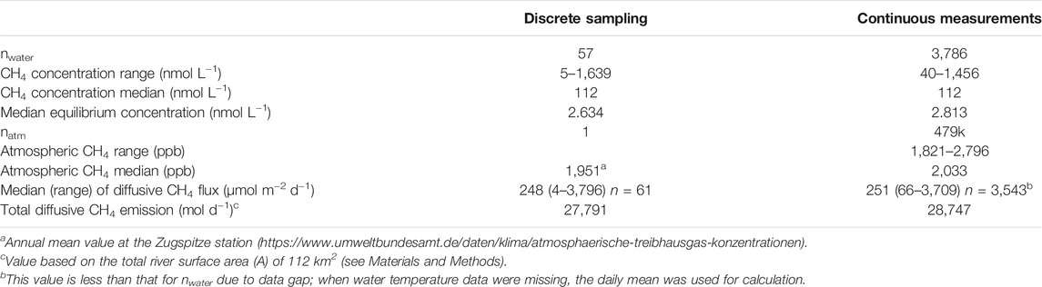
TABLE 1. Comparison of the discrete and continuous measurements of dissolved and atmospheric CH₄ and resulting CH₄ emission estimates.

In the Elbe channel near the Czech border (near km-4), CH₄ concentration was rather high (250 nmol L⁻¹). In the first 120 km, dissolved CH₄ concentration decreased steadily, albeit without marked variability (50–100 nmol L⁻¹) (Figure 2A). In the middle part, dissolved CH₄ concentration fluctuated between 50 and 110 nmol L⁻¹. In this part of the river, we observed large variability, with several distinct small peaks (Figure 3). There was a clear increase in CH₄ concentration to approximately 200 nmol L⁻¹ after km-430 (Figure 2A). Starting from Elbe km-560, CH₄ concentrations increased further toward the weir Geesthacht, reaching very high values up to 1,000 nmol L⁻¹ (Figure 2A).

FIGURE 2

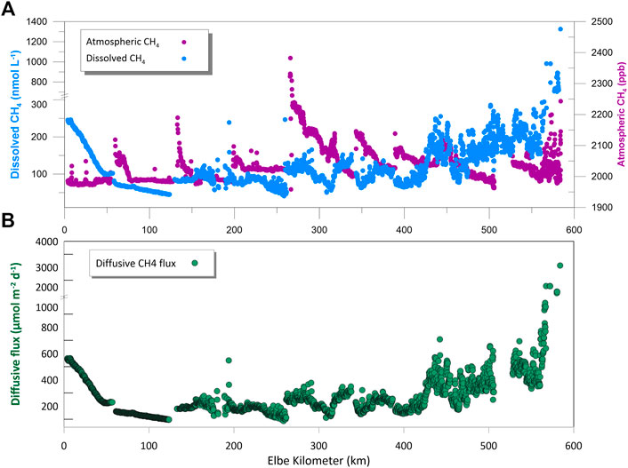
FIGURE 2. Atmospheric (ppb) and dissolved CH₄ (nmol L⁻¹) concentration (A) and diffusive CH₄ emissions (µmol m⁻² d⁻¹) versus river km (B) Only data obtained when the vessel was moving at the speed of >4 kn were considered; tributaries were excluded.

FIGURE 3

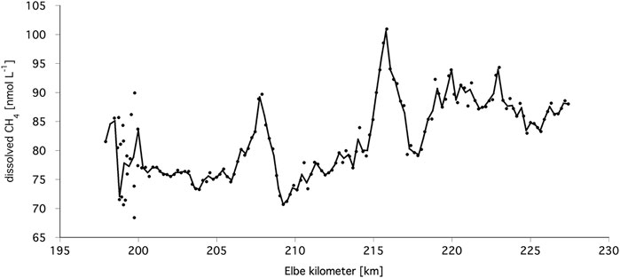
FIGURE 3. Small-scale heterogeneity of dissolved CH₄ along a selected reach around km-210. Data from Figure 2 were used; interpolated line is shown.

The median diffusive CH₄ flux from the water to atmosphere along the Elbe course was 251 μmol m⁻² d⁻¹, ranging from 66 to 3,709 μmol m⁻² d⁻¹ (Table 1; Figure 2B). The distribution of diffusive flux along the river reflected the distribution of CH₄ concentration, with the maxima at harbors, near the shore, and upstream of the weir (Supplementary Figure S4). The comparison of calculations based on the continuous measurements of dissolved and atmospheric CH₄ and water temperature versus the calculations based on single water samples and the overall German atmospheric CH₄ concentration revealed near identical median values but narrower ranges (Table 1).

3.2 Atmospheric CH₄

The mean atmospheric CH₄ concentration along the Elbe course was 2,034 ± 54 ppb (Figure 2A). The time series showed a distinct sawtooth pattern. Apparently, the deviation from the atmospheric baseline is related to the time of day, with more or less increased concentrations in the early morning hours, followed by a slow decrease to the normal conditions during the day.

To analyze the temporal behavior of atmospheric gas concentrations and distinguish between temporal and spatial patterns, longer observation periods at a fixed location were required. For that purpose, we used continuous measurements during the night-time stops in harbors, for instance, a 12-h stop at Elbe km-200 near Dessau. A substantial increase of approximately 15% in the mixing ratio for both gases during the night may be attributed to the still active (and more or less stable) emission sources, consistent with atmospheric accumulation processes due to low dynamics in the near-surface layers (wind velocity <2 m s⁻¹; data from the Elster weather station, Elbe).

Furthermore, the diurnal cycle (Figure 4) reflected the causes of the observed patterns of and jumps in atmospheric CH₄ concentrations depicted in Figure 2A. The atmospheric CH₄ data appeared to be clearly affected by the diurnal wind situation. After a calm night with low winds in the morning hours, extreme increases in atmospheric CH₄ concentrations were observed in the harbors. Moreover, the cruise often started with higher CH₄ concentrations in the morning hours compared to the latest values measured on the previous day at the same location. In the further course of the day, the values gradually stabilized, resulting in the typical sawtooth pattern, as shown in Figure 2A. Hence, to use atmospheric CH₄ measurements as an indicator of potential emission sources, the knowledge of meteorological conditions and the diurnal cycle at selected locations is necessary.

FIGURE 4

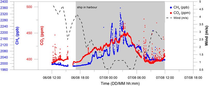
FIGURE 4. Variability in the atmospheric greenhouse gas concentrations during a diurnal cycle compared to the wind conditions measured in the surrounding at Elbe km-200. Wind data were obtained from https://www.timeanddate.de/wetter/deutschland.

In addition to this regular pattern, some locations with increased atmospheric CH₄ concentrations were detected during the continuous measurements. In particular, while staying in harbors or passing larger urban areas (such as the cities of Dresden or Magdeburg), increased CH₄ concentrations were observed. Interestingly, according to the elevated dissolved CH₄ concentrations, zones with increased atmospheric values were measured (e.g., upstream of the weir Geesthacht, at km-560: maximum concentration = 2,250 ppb).

3.3 Small-Scale Variability

We also observed small-scale variability of dissolved CH₄. A typical mid-river section (Figure 3) exemplified some noise but also distinct concentration peaks. For instance, at km-207 and km-215, two small peaks were observed with an increase from 75 to 90 nM and from 80 to 100 nM, respectively. More such small peaks were observed from km-260 to km-300 (not shown).

These locally elevated CH₄ concentrations are difficult to explain. A possible reason is that the vessel occasionally approached one of the river sides, where concentrations were higher. However, there was no correlation between the distance of the vessel from the central waterway and the dissolved CH₄ concentration. Thus, the peaks cannot be explained by lateral vessel movements. In addition, CH₄ concentration was not correlated with flow velocities above 0.8 m s-¹ (Supplementary Figure S5).

3.4 Lateral Variations

CH₄ concentrations in the water samples taken near the shore were significantly higher than those in the middle of the river (Supplementary Figure S6, Wilcoxon rank sign test, paired data, n = 19, p = 0.01 for right shore vs. middle and p = 0.05 for left shore versus middle). The mean CH₄ concentration at the 18 sites was 300 ± 393 nmol L⁻¹ near the shore and 228 ± 350 nmol L⁻¹ in the middle, indicating a difference of 32%.

Based on high-resolution measurements, we observed either no difference (Schmilka, Figure 5A, 31%), a symmetric distribution of the lateral increase (Rogätz, Figure 5B, 25%), a one-sided increase (Werben, Figure 5C, 31%), or a linear increase (13%) in dissolved CH₄ in the lateral transects. Elevated CH₄ concentrations near the shore were more pronounced and more variable in the lower reaches of the river (Supplementary Figure S6). We compared the different patterns of the lateral CH₄ distribution in Schmilka (no difference), Rogätz (symmetric), and Werben (one-sided) based on the aerial photographs of the sites (provided by Googpe Earth Pro for 24 June 2016; 6 August 2020; and 15 September 2016). In Schmilka, no obstacles were noted at the shore line. Meanwhile, groins were visible on both sides in Rogätz and in Werben only at the left river shore.

FIGURE 5

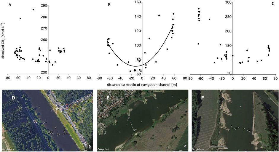
FIGURE 5. Dissolved CH₄ concentration at lateral transects in Schmilka (A and D, km-4) Rogätz (B and E, km-351) and Werben (C and F, km-422). Aerial photographs were retrieved from Google Earth Pro, dots indicate the ship’s position.

3.5 Hotspots

The highest dissolved CH₄ concentrations were recorded in the harbors (Dresden, Mühlberg, Leopoldshafen, Niedgripper Schleuse, Wittenberg, and Dömitz), with a median of 828 nM, ranging from 284 to 2,136 nM. Accordingly, the diffusive flux in the harbors was nearly six times higher than that in the river itself, with a median of 1,655, ranging from 806 to 3,010 μmol m⁻² d⁻¹.

Additionally, elevated CH₄ concentrations were noted as the course approached Geesthacht weir on August 12 (Figure 6). Intermediate CH₄ concentrations (minimum = 154 nM) were recorded until 24 km before the weir, and the value increased toward the weir, reaching the maximum concentration of 1,127 nM (km-555 to km-590). Conductivity and temperature slightly increased toward the weir, while chlorophyll and turbidity decreased. The diffusive flux of CH₄ increased toward the weir, from values below 700 μmol m⁻² d⁻¹ at Elbe km < 567 to values exceeding 1,500 μmol m⁻² d⁻¹ at Elbe km > 576.

FIGURE 6

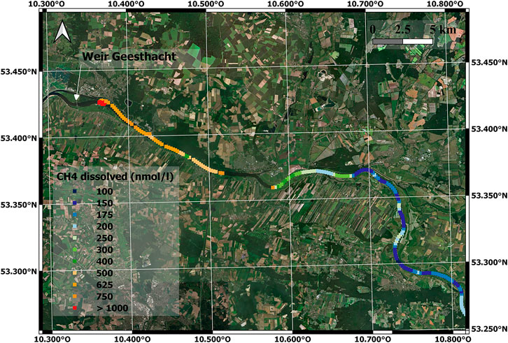
FIGURE 6. Dissolved CH₄ concentration upstream of the weir Geesthacht. Map base: Bing Aerial.

Likewise, atmospheric CH₄ concentrations also increased toward the weir (Figure 7), although no direct correlation with dissolved CH₄ concentration or diffusive CH₄ flux was noted.

FIGURE 7

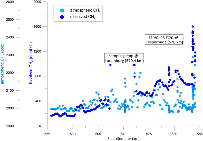
FIGURE 7. Atmospheric CH₄ and dissolved CO₂ and CH₄ concentrations upstream of the weir Geesthacht.

3.6 Tributaries

Tributaries showed little effect on CH₄ concentrations in the main river. CH₄ concentrations downstream of tributary inflows were similar to the concentrations upstream (Table 2; Figure 8). Discharge of Havel was about 2% of the Elbe discharge. Compared with the value in the upstream region of Elbe (165 nM), CH₄ concentration in the upstream region of Havel was higher (256 nM). However, in the downstream region, CH₄ concentration rapidly decreased within 1.2 km (149 nM) (Table 2 and Figure 8). The CH₄ concentration predicted assuming conservative mixing was 167 nM. Similar trends of a negligible influence were also noted in the other tributaries (Supplementary Figures S7, S8 and Table 2).

TABLE 2

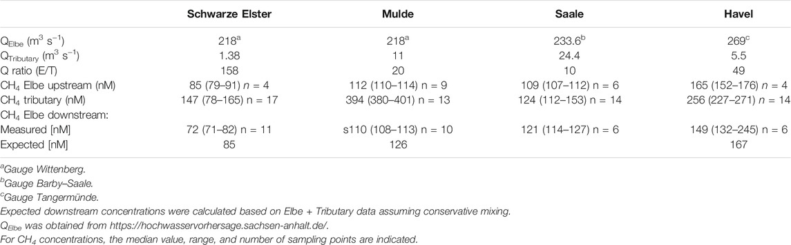
TABLE 2. CH₄ budget at tributary inflows.

FIGURE 8

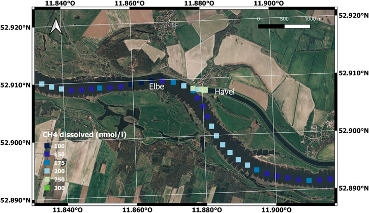
FIGURE 8. CH₄ concentration at the mouth of Havel. Map base: Bing Aerial.

Interestingly, we observed a small hotspot with elevated CH₄ approximately 3 km upstream of the mouth of Havel (Figure 8). Along a reach of ∼2.5 km, CH₄ concentrations were nearly 1.7 times elevated. A detailed inspection of the cruise track revealed that the vessel had been steaming close to an area of large groin fields on the left-hand shore (Figure 8).

3.7 Flux and Upscaling

We applied a weighted approach to calculate the total diffusive flux of CH₄ from Elbe to the atmosphere, taking into account the fact that the width of the river increases from the Czech border toward Geesthacht weir (112 m at km-10–282 m at km-497), with a final increase in CH₄ concentration towards the weir. The weighted approach revealed a total area of 112 km², resulting in the emission of 28,747 mol CH₄ d⁻¹ (Table 1), which is equivalent to 0.46 t CH₄ d⁻¹. The calculation of total daily emissions based on discrete water sampling data revealed a similar value (0.43 t CH₄ d⁻¹). Thus, the spatial resolution of discrete sampling was sufficient to estimate correct total emission.

To evaluate the benefit of high-resolution CH₄ data for upscaling, we subsampled our continuous dataset of dissolved CH₄ assuming sampling every 10, 20, 50, or 100 km. The “all” dataset considered only sampling at the river, excluding harbors, and no transects, resulting in a total of 2,740 data points. The starting point at km-3 and endpoint at km-584 were included in all cases. As a result, the following average values of dissolved CH₄ and number of data points were recorded: 137 ± 116 nM (std error = 2%) and n = 2,665 for the “all” dataset; 148 ± 183 nM (std error = 24%) and n = 59 for the every 10 km dataset; 158 ± 231 nM (std error = 43%) and n = 29 for the every 20 km dataset; 209 ± 341 nM (std error = 95%) and n = 13 for the every 50 km dataset; and 290 ± 462 nM (std error = 175%) and n = 7 for the every 100 km dataset, respectively. The average values increased from the “all” dataset (137 nM) toward the every 100 km dataset (290 nM); however, the standard deviation and standard error also increased markedly. As shown in Figure 9, with the example of the “every 50 km” data set, the background and median values could be easily covered with less frequent sampling. However, the peaks and extremes could be rarely covered.

FIGURE 9

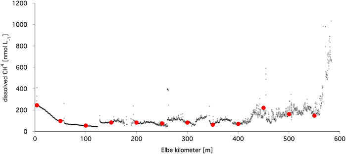
FIGURE 9. Comparison between the continuously measured dissolved CH₄ concentration (small black dots) and the concentration (red circles) at every 50 km.

The relevance of different sampling densities to the calculation of diffusive flux was estimated by determining the area under the curve of the diffusive flux along Elbe. The cumulative diffusive flux along Elbe, as measured with continuous sampling, was 177 mol m⁻¹ d⁻¹. With sampling every 10, 20, 50, and 100 km, the cumulative diffusive fluxes were mostly higher at 174, 183, 191, and 255 mol m⁻¹ d⁻¹, respectively. Sampling at 10 and 20 km yielded comparable results to continuous sampling. However, inadequate sampling at 50 and 100 km resulted in the overestimation of diffusive flux by 8–44%.

4 Discussion

The Elbe River was consistently oversaturated with CH₄ (related to water in equilibrium with atmospheric CH₄), rendering it a steady source of the emission of this GHG to the atmosphere. This result is consistent with literature (Stanley et al., 2016) and supports the view that in addition to small streams, which receive CH₄ from riparian soils (Leng et al., 2021), larger rivers must also be considered CH₄ sources. Our emission estimate of 251 μmol m⁻² d⁻¹ (153 t y⁻¹ in total) is almost double than a previous estimate (131 μmol m⁻² d⁻¹ or 97 t y⁻¹, Matoušů et al., 2019). However, the estimated flux from Elbe was comparable to that recorded from other large German rivers, including Rhine (119 μmol m⁻² d⁻¹; Wilkinson et al., 2019) and Danube (209–370 μmol m⁻² d⁻¹; Canning et al., 2021; Maier et al., 2021). This study was conducted in August 2020; therefore, seasonal differences in water discharge, water temperature and CH₄ concentrations were not considered.

4.1 Methods

The comparison of CH₄ emission calculation based on either continuous or discrete data proved that conventional discrete sampling is sufficient to scale up emissions to the entire river. Furthermore, we did not observe a diurnal pattern of CH₄ concentrations in the water, indicating that the time of day need not be considered in discrete sampling schemes. Thus, continuous CH₄ data from a river cruise are not affected by short term temporal fluctuations and useful to identify the spatial patterns of this GHG.

Typically, a constant atmospheric mixing ratio is used to calculate the concentration gradient at the water–atmosphere interface. Although we observed some variability in atmospheric CH₄, this had a minor effect on flux calculation and upscaling. The median CH₄ concentration was 4% higher than the reference measurements at Zugspitze. At Germany’s highest peak, the measured values are particularly representative of the background pollution of the atmosphere and largely unaffected by local sources (https://www.umweltbundesamt.de/daten/klima/atmosphaerische-treibhausgas-konzentrationen). Using that value as the reference atmospheric concentration for flux calculations, the median CH₄ flux would be 251 μmol m⁻² d⁻¹, which is identical to the value we obtained based on the in-situ data. Therefore, for the German Elbe, continuous measurements of atmospheric CH₄ are not required to obtain a reliable flux estimate.

The conversion of concentration data to diffusive emission requires the knowledge of gas transfer velocity (K_600, the gas transfer velocity for CO₂ at 20°C). In the present study, we did not measure K but used previously published data calculated from simultaneous flux and concentration measurements (Matoušů et al., 2019). Our K₆₀₀ of 2.35 m d⁻¹ for German Elbe is similar to the values reported for other large rivers, including Danube (median = 0.69, range = 0.2–3.4 m d⁻¹) (Maier et al., 2021). A similar K₆₀₀ of 2.53 m d⁻¹ was obtained using the standard empirical calculation of K₆₀₀ based on flow velocity and slope (Raymond et al., 2012). Although the use of a constant K₆₀₀ for the entire river would surely introduce some bias, we consider the possible error to be rather small. Flow conditions were rather uniform along the river channel. The mean flow velocity during the cruise was 0.9 ± 0.2 m s⁻¹ (Supplementary Figure S5) based on data derived from a river model (Andreas Schöl, pers. com.). Thus, as K₆₀₀ fluctuated within a rather narrow range, the effect of K₆₀₀ variations on total CH₄ emission estimates should be minor. An exception might be the reach directly upstream of the weir at Geesthacht, where the flow velocity was ∼0.2 m s⁻¹ [K₆₀₀ = 2.1, according to Raymond et al. (2012)], and the use of a constant K₆₀₀ (2.32) may have slightly overestimated diffusive emissions.

However, while the longitudinal heterogeneities of K₆₀₀ probably had a minor impact on total CH₄ emissions, this may not be true for lateral transects. Previous comparisons of K₆₀₀ in the middle of the river and near the shore along Magdeburg have indicated approximately 40% lower K₆₀₀ values near the river banks (Koschorreck, unpublished data). However, a lower K₆₀₀ near the shore may be balanced by a higher K₆₀₀ at groin heads, where water flow is typically turbulent. Thus, small-scale quantification of K₆₀₀ using drifting floating chambers (Lorke et al., 2015) is essential to better assess gas transfer velocities at large rivers.

Our data show that lateral heterogeneity is definitely relevant to the assessment of dissolved CH₄ concentrations. Here, we emphasize the effects of measurement strategies. First, our longitudinal dataset may be affected by the exact position of the vessel in the river during the cruise. Second, when obtaining discrete samples from a river for CH₄ quantification, it is important to sample water from not only the middle of the river but also sides—a fact already known for the measurement of other water parameters (Weigold and Baborowski 2009).

Furthermore, the lateral extension (width) of the river must also be considered when CH₄ emissions are scaled up to the entire river. For instance, we compared two sites (km-75 versus km-311) with similar diffusive CH₄ fluxes (146 μmol m⁻² d⁻¹) but with different widths (132 versus 189 m). At the wider site, the total diffusive flux was approximately 1.5 times higher (28 versus 19 mol d⁻¹). Overlooking different widths and simply applying the mean flux to the entire river area would assign greater weight to measurements in the upstream area (narrower), thus underestimating the total emissions. As Elbe becomes broader toward Geesthacht and the CH₄ concentrations increase, the total CH₄ flux of this area is high both due to high CH₄ concentration and large surface area.

This study was conducted at mean water level. It is currently unclear what influence the water level has on the flow conditions at the groins. Further seasonal studies are needed here.

4.2 Hotspot Occurrence and Extension

Since the flow velocity of Elbe was rather uniform (with the exception of reaches upstream the weir), any pronounced deviation from the baseline CH₄ concentration should be caused by the changes in source strength. However, as our data show it is not trivial to distinguish a point source of CH₄ from a “hot moment,” which may create CH₄ plumes. We observed different shapes of CH₄ peaks during our cruise which we conceptualize in Figure 10. A point source should result in a stationary hotspot with declining concentration downstream due to outgassing. Meanwhile, a “hot moment” would result in a parcel of water with elevated CH₄ concentration, which moves downstream, losing CH₄ to the atmosphere on its way. Thus, information on the source of elevated CH₄ can be gained by analyzing continuous CH₄ concentration dataset, as discussed below.

FIGURE 10

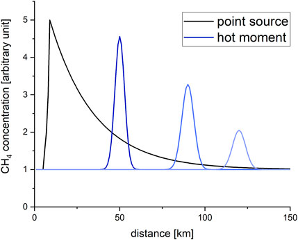
FIGURE 10. Shape of a hypothetical CH₄ hotspot depending on its origin. The point source curve was calculated as described by Crawford et al. (2014), assuming k₆₀₀ = 2.32 m d⁻¹, water depth = 1 m, and flow velocity = 0.72 m s⁻¹. The blue lines indicate the downstream movement of a CH₄ plume created by a “hot moment.”

4.2.1 Weirs and Harbors as Hotspots

Weirs affect CH₄ concentrations both in the upstream and downstream reaches. Thus, weirs act as a point source. The higher CH₄ concentration at the start of our cruise was probably caused by the weir at Usti, approximately 40 km upstream of our starting point in Schmilka. This speculation is supported by our observation of elevated CH₄ at Geesthacht weir as well as earlier observations (Matoušů et al., 2019). Assuming that CH₄ oxidation is slow [6–10 times slower than diffusive loss (Heilweil et al., 2016; Matoušů et al., 2019)], CH₄ outgassing must be the major loss process and the impact of a weir as a point source should be evident up to 100 km downstream (Figure 10). This is consistent with our observation of “normal” concentrations nearly 60 km downstream of Schmilka, which is 100 km downstream of the weir. Thus, in addition to the dammed section, weirs increase CH₄ concentrations also in reaches downstream of the weir.

As expected, CH₄ concentrations and emissions were high upstream of the Geesthacht weir (with emissions of >1,500 μmol m⁻² d⁻¹ at the weir versus the median of only 251 μmol m⁻² d⁻¹ for the entire river). The surface area before the weir (km > 576) is ∼4 million m² (estimated based on a Google Earth Pro image), and as the diffusive flux was high, the region accounted for 28% to the total diffusive CH₄ emissions from Elbe. The trapping of sediments upstream of river dams triggers high CH₄ production in the sediment (Maeck et al., 2013), resulting in extreme CH₄ emissions (DelSontro et al., 2010). At such sites, CH₄ emissions are typically dominated by ebullition—a process not considered in the present study. Thus, at least in the dammed section, our CH₄ emission estimation based solely on diffusion probably underestimated the actual value. While continuous CH₄ concentration measurements are suitable to detect CH₄ concentration hotspots, they are not suitable to quantify emissions at hotspots where ebullition occurs. However, ebullition also increases CH₄ concentration in the water due to CH₄ loss from rising bubbles (DelSontro et al., 2010). Thus, we believe that continuous CH₄ concentration measurements allow the detection of sites with intensive ebullition.

At harbors, we observed high diffusive fluxes, which were approximately 6 times greater than in the river itself. These observations corroborate the results reported by Matoušů et al. (2019). In the harbor basins with mostly stagnant water, organic material accumulates, resulting in higher CH₄ concentrations and diffusive fluxes. We estimated the areas of the harbors Dresden, Mühlberg, Dessau, Niegripper Schleuse, Wittenberg and Dömitz using Google Earth Pro and calculated a total area of 404,974 m². However, as their respective areas were small, these harbors accounted for only 2% to the total flux in Elbe. Thus, the river itself accounts for 70% of the diffusive flux. These flux estimates for harbors can be considered the maximum values, since we used the same K for harbors as that for the flowing river. These results were consistent with our harbor flux estimates based on atmospheric CH₄ accumulation during the night, which showed that CH₄ fluxes in the harbor and river were quite similar. Thus, in harbors, high CH₄ concentrations are counterbalanced by low K values and may be neglected from the quantification of total CH₄ emissions from the river.

4.2.2 Hot Moments and Small-Scale Variability

We frequently observed small peaks of dissolved CH₄ for which we could find no straightforward explanation (Figure 3). Interestingly, we observed these small peaks only in areas with groins. As discussed below, groin fields are the possible sources of CH₄. Between the groin heads, the shear stress of the main current leads to an energy input into the groin fields, resulting in eddies detaching from the groin heads. Furthermore, they promote energy and mass exchange between the main and the groin field flow (Kleinwächter et al., 2017). In the context of the present study, this implies that at the head of the groins, CH₄-rich eddies were released, which then traveled along Elbe, becoming smaller with time (Figure 10).

In our analysis, we probably overestimated the size of these small peaks because the vessel was moving with the current. When the vessel steaming downstream at ∼3.6 m s⁻¹ was passing a CH₄ plume drifting at 0.9 m s⁻¹ in the same direction, it likely stayed longer in the plume than when the water was not moving. As a result, the spatial extent of these plumes may have been overestimated.

4.2.3 Tributaries

The inflow of four tributaries (Schwarze Elster, Mulde, Saale, and Havel) did not markedly increase CH₄ concentrations in the main river below the confluence, even though CH₄ concentration within the tributaries were significantly higher than that in the mainstream, as also observed in a similar study in 2017 (Matoušů et al., 2019). This is not surprising considering the lower relative discharge of the tributaries than that of Elbe (Table 2). Only Saale contributed a considerable amount of water (10% of the Elbe discharge), but its CH₄ concentrations were only marginally elevated compared to those in Elbe.

Another possible explanation for the minor influence of the tributaries is that the vessel mainly measured concentrations in the middle of the river. Thus, we may have missed the plumes of the tributaries, when their input was flowing parallel to the shore. For Saale, where conductivity is elevated, water mainly flows along the left shoreline and complete mixing occurs only after 100 km (Kamjunke et al., 2021). In future studies, the inflow of tributaries should be better followed along the shore line.

Low contribution to riverine CH₄ is probably also true for backwaters, which may exhibit extremely high CH₄ concentrations (Staniek 2019). In River Danube, CH₄ exchange between floodplain waters and the river was driven by hydrology, and significant amounts of CH₄ were flushed into the river when the water level was lowering (Sieczko et al., 2016). However, under stagnant low-water conditions, as in the present study, most floodplain waters are disconnected from the river, with little water exchange.

4.2.4 Atmospheric Measurements as a Tool for Hotspot Detection

The measurement of CH₄ concentrations in the atmosphere directly above the water surface has been used to identify the hotspots of CH₄ emissions and even calculate emission rates (Dunbabin and Grinham 2017). We observed elevated atmospheric CH₄ concentrations in harbors and in reaches upstream of a weir, confirming that atmospheric measurements can be useful to identify emission hotspots. However, the calculation of fluxes based on our atmospheric CH₄ data was only possible under specific environmental conditions. Our analyses revealed a considerable effect of diurnal meteorological conditions on the atmospheric CH₄ mixing ratio, which prevented quantitative interpretation with respect to aquatic emissions. As an exception, measurements at night, when the vessel was anchored in the harbors, showed elevated atmospheric CH₄. Using a virtual open chamber approach (Barkwith et al., 2020), an emission rate of 8.4 μmol m⁻² h⁻¹ (=202 μmol m⁻² d⁻¹) was calculated in the quiet nighttime hours. This value is close to the diffusive flux of 251 μmol m⁻² d⁻¹ (Table 1). In daylight hours, when the wind conditions were more complex and when the vessel was cruising along the river, atmospheric data were rather stable and did not allow for the tracking of small-scale variability and spots with locally elevated aquatic CH₄ concentrations.

4.3 Large-Scale Patterns and Effects of Groins

In addition to the above hotspots, we observed interesting large-scale patterns. Before km-130, the variability of dissolved CH₄ was rather low. Despite the longitudinal trend, we did not observe small-scale fluctuations. Further, there was an evident change in dissolved CH₄ around km-130. Notably, this observation coincided with the first appearance of groins. To improve navigability, groins have been constructed all along the downstream reaches of Elbe from km-122. These groin fields give rise to a high spatiotemporal diversity of sedimentation regimes (Henning and Hentschel 2013).

The hypothesis that groins increase the variability of riverine CH₄ was supported by our lateral transect data, which showed elevated CH₄ concentrations near the shore only in the presence of groins. This is plausible because groins create areas of reduced flow velocity, resulting in the sedimentation of suspended particles (Pusch and Fischer 2006). These accumulated sediments act as the sites of intensive organic matter mineralization and, probably, methanogenesis (Schwartz and Kozerski 2003). Assuming that groin fields are the relevant sources of CH₄, the CH₄ concentrations in the river may be regulated by 1) CH₄ production in a respective groin field and 2) water exchange between the groin field and the middle of the river.

The lateral variability of CH₄ concentration was more pronounced in the downstream reaches of the river (Supplementary Figure S6), implying higher CH₄ production in these downstream reaches or lower water exchange between the banks and middle of the river, resulting in CH₄ accumulation in the groin fields. The second explanation is more plausible given the greater width of the river (Supplementary Figure S1), combined with lower flow velocity. Evidently, the presence of groin fields increases riverine CH₄ concentrations, although the magnitude of this effect depends on site conditions.

It is well known that damming increases CH₄ emissions from rivers (Maeck et al., 2013). We show in this study that damming is not the only mechanism by which human alterations increase riverine CH₄ emissions. We conclude that the construction of groins is an additional mechanism by which anthropogenic modifications significantly increase CH₄ emissions from rivers.

5 Conclusion

Besides the conventional assessments of spatial heterogeneity in streams based on discrete sampling, we presented data from a new approach continuously investigating large-scale patterns and hotspots of elevated CH₄ concentrations along the Elbe River. We observed large-scale patterns of GHG concentrations both along the river course and in specific regions with elevated dissolved CH₄ concentrations, such as harbors, some tributaries and the weir. The River Elbe was consistently oversaturated with CH₄ (related to water in equilibrium with atmospheric methane) and had to be considered as a CH₄ source with an emission rate estimated at 251 μmol m⁻² d⁻¹.

High-spatial resolution measurements of dissolved CH₄ in the River Elbe revealed that weirs increased CH₄ concentrations not only upstream, but also downstream of a weir. At these hotspots not only elevated CH₄ concentrations in the water but also in the atmosphere were observed, confirming that atmospheric measurements can be useful to identify emission hotspots.

The inflow of four tributaries did not significantly increase CH₄ concentrations in the main river below the confluence. However, to fully assess the impact of tributaries on riverine CH₄ spatially resolved sampling downstream of the confluence areas is necessary.

Groin fields appeared to be an unexpected but important source of high small-scale variability. We could clearly distinguish between river reaches without groins and lower and constant CH₄ concentration and river reaches with groins with a high variability of dissolved CH₄. Thus, the CH₄ concentration in the river is regulated by a complex interplay of 1) CH₄ originating from upstream reaches, 2) CH₄ production in a respective groin field, and 3) water exchange between the groin field and the middle of the river. These interactions result in significant lateral CH₄ concentration profiles with higher dissolve CH₄ concentrations near to the shore as well as in hitherto unknown small scale CH₄ concentration fluctuations along the river. Future work aiming to quantify CH₄ emissions from rivers needs to take into account this variability.

The direct comparison of our discrete and continuous measurements proved that conventional discrete sampling is sufficient to estimate an upscaled methane emission rate for the entire river. However, our data also clearly show the importance of the acquisition of regions with small-scale anomalies based on high resolution sampling strategies. The here proposed continuous sampling is valuable to survey the entire river system or at least the vulnerable regions, which can be of great relevance in case of extreme hydrological events.

Data Availability Statement

The datasets presented in this study can be found in the pangea repository at the following address: https://doi.pangaea.de/10.1594/PANGAEA.939900.

Author Contributions

All authors listed have made a substantial, direct, and intellectual contribution to the work and approved it for publication.

Funding

This study was part of the Helmholtz Program Changing Earth, ST4.1: “Fluxes and transformation of energy and matter in and across compartments;” and ST5.2 “Water resources and environment.” We acknowledge funding from the Helmholtz Association in the framework of the Helmholtz funded observation system MOSES (Modular Observation Solutions for Earth Systems) and from the Initiative and Networking Fund of the Helmholtz Association through the project “Digital Earth” (funding code ZT-0025).

Conflict of Interest

The authors declare that the research was conducted in the absence of any commercial or financial relationships that could be construed as a potential conflict of interest.

Publisher’s Note

All claims expressed in this article are solely those of the authors and do not necessarily represent those of their affiliated organizations, or those of the publisher, the editors and the reviewers. Any product that may be evaluated in this article, or claim that may be made by its manufacturer, is not guaranteed or endorsed by the publisher.

Acknowledgments

We thank Sven Bauth, Erik Evers, Heike Goretzka, Hannah Jebens, and Ute Link, and for help during field and laboratory work.

Supplementary Material

The Supplementary Material for this article can be found online at: https://www.frontiersin.org/articles/10.3389/fenvs.2022.833936/full#supplementary-material

References

Barkwith, A., Beaubien, S. E., Barlow, T., Kirk, K., Lister, T. R., Tartarello, M. C., et al. (2020). Using Near-Surface Atmospheric Measurements as a Proxy for Quantifying Field-Scale Soil Gas Flux. Geosci. Instrum. Method. Data Syst. 9 (2), 483–490. doi:10.5194/gi-9-483-2020

CrossRef Full Text | Google Scholar

Bastviken, D., Tranvik, L. J., Downing, J. A., Crill, P. M., and Enrich-Prast, A. (2011). Freshwater Methane Emissions Offset the continental Carbon Sink. Science 331 (6013), 50. doi:10.1126/science.1196808

PubMed Abstract | CrossRef Full Text | Google Scholar

Canning, A., Wehrli, B., and Körtzinger, A. (2021). Methane in the Danube Delta: the Importance of Spatial Patterns and Diel Cycles for Atmospheric Emission Estimates. Biogeosciences 18 (12), 3961–3979. doi:10.5194/bg-18-3961-2021

CrossRef Full Text | Google Scholar

Crawford, J. T., Lottig, N. R., Stanley, E. H., Walker, J. F., Hanson, P. C., Finlay, J. C., et al. (2014). CO₂ and CH₄ Emissions from Streams in a Lake-Rich Landscape: Patterns, Controls, and Regional Significance. Glob. Biogeochem. Cycles 28 (3), 197–210. doi:10.1002/2013gb004661

CrossRef Full Text | Google Scholar

DelSontro, T., McGinnis, D. F., Sobek, S., Ostrovsky, I., and Wehrli, B. (2010). Extreme Methane Emissions from a Swiss Hydropower Reservoir: Contribution from Bubbling Sediments. Environ. Sci. Technol. 44 (7), 2419–2425. doi:10.1021/Es9031369

PubMed Abstract | CrossRef Full Text | Google Scholar

Donelan, M. A., Drennan, W. M., Saltzman, E. S., and Wanninkhof, R. (2002). Gas Transfer at Water Surfaces. Washington, USA: American Geophysical Union. doi:10.1029/GM127

CrossRef Full Text | Google Scholar

Dunbabin, M., and Grinham, A. (2017). Quantifying Spatiotemporal Greenhouse Gas Emissions Using Autonomous Surface Vehicles. J. Field Rob. 34 (1), 151–169. doi:10.1002/rob.21665

CrossRef Full Text | Google Scholar

Gålfalk, M., Olofsson, G., Crill, P., and Bastviken, D. (2016). Making Methane Visible. Nat. Clim Change 6, 426–430. doi:10.1038/nclimate2877

CrossRef Full Text | Google Scholar

Gonzalez-Valencia, R., Magana-Rodriguez, F., Gerardo-Nieto, O., Sepulveda-Jauregui, A., Martinez-Cruz, K., Walter Anthony, K., et al. (2014). In Situ measurement of Dissolved Methane and Carbon Dioxide in Freshwater Ecosystems by off-Axis Integrated Cavity Output Spectroscopy. Environ. Sci. Technol. 48 (19), 11421–11428. doi:10.1021/es500987j

PubMed Abstract | CrossRef Full Text | Google Scholar

Heilweil, V. M., Solomon, D. K., Darrah, T. H., Gilmore, T. E., and Genereux, D. P. (2016). Gas-Tracer Experiment for Evaluating the Fate of Methane in a Coastal Plain Stream: Degassing versus In-Stream Oxidation. Environ. Sci. Technol. 50 (19), 10504–10511. doi:10.1021/acs.est.6b02224

PubMed Abstract | CrossRef Full Text | Google Scholar

Henning, M., and Hentschel, B. (2013). Sedimentation and Flow Patterns Induced by Regular and Modified Groynes on the River Elbe, Germany. Ecohydrol. 6 (4), 598–610. doi:10.1002/eco.1398

CrossRef Full Text | Google Scholar

Kamjunke, N., Rode, M., Baborowski, M., Kunz, J. V., Zehner, J., Borchardt, D., et al. (2021). High Irradiation and Low Discharge Promote the Dominant Role of Phytoplankton in Riverine Nutrient Dynamics. Limnol. Oceanogr. 66, 2648–2660. doi:10.1002/lno.11778

CrossRef Full Text | Google Scholar

Karion, A., Sweeney, C., Pétron, G., Frost, G., Michael Hardesty, R., Kofler, J., et al. (2013). Methane Emissions Estimate from Airborne Measurements over a Western United States Natural Gas Field. Geophys. Res. Lett. 40 (16), 4393–4397. doi:10.1002/grl.50811

CrossRef Full Text | Google Scholar

Kleinwächter, M., Schröder, U., Rödiger, S., Hentschel, B., and Anlauf, A. (2017). Alternative Buhnenformen in der Elbe - hydraulische und ökologische Wirkungen. Kapitel 3: Buhnen an der Elbe und ihre Umgestaltung. Stuttgart: Schweizerbart.

Google Scholar

Koschorreck, M., Prairie, Y. T., Kim, J., and Marcé, R. (2021). Technical Note: CO₂ Is Not like CH₄ - Limits of and Corrections to the Headspace Method to Analyse pCO₂ in Fresh Water. Biogeosciences 18 (5), 1619–1627. doi:10.5194/bg-18-1619-2021

CrossRef Full Text | Google Scholar

Leng, P., Kamjunke, N., Li, F., and Koschorreck, M. (2021). Temporal Patterns of Methane Emissions from Two Streams with Different Riparian Connectivity. J. Geophys. Res. Biogeosci. 126 (8), e2020JG006104. doi:10.1029/2020JG006104

CrossRef Full Text | Google Scholar

Lorke, A., Bodmer, P., Noss, C., Alshboul, Z., Koschorreck, M., Somlai-Haase, C., et al. (2015). Technical Note: Drifting versus Anchored Flux chambers for Measuring Greenhouse Gas Emissions from Running Waters. Biogeosciences 12 (23), 7013–7024. doi:10.5194/bg-12-7013-2015

CrossRef Full Text | Google Scholar

Maeck, A., DelSontro, T., McGinnis, D. F., Fischer, H., Flury, S., Schmidt, M., et al. (2013). Sediment Trapping by Dams Creates Methane Emission Hot Spots. Environ. Sci. Technol. 47 (15), 8130–8137. doi:10.1021/es4003907

PubMed Abstract | CrossRef Full Text | Google Scholar

Maier, M.-S., Teodoru, C. R., and Wehrli, B. (2021). Spatio-temporal Variations in Lateral and Atmospheric Carbon Fluxes from the Danube Delta. Biogeosciences 18 (4), 1417–1437. doi:10.5194/bg-18-1417-2021

CrossRef Full Text | Google Scholar

Mallast, U., Staniek, M., and Koschorreck, M. (2020). Spatial Upscaling of CO₂ Emissions from Exposed River Sediments of the Elbe River during an Extreme Drought. Ecohydrology 13, e2216 (6). doi:10.1002/eco.2216

CrossRef Full Text | Google Scholar

Matoušů, A., Rulík, M., Tušer, M., Bednařík, A., Šimek, K., Bussmann, I., et al. (2019). Methane Dynamics in a Large River: a Case Study of the Elbe River. Aquat. Sci. 81 (1), 12. doi:10.1007/s00027-018-0609-9

CrossRef Full Text | Google Scholar

Pusch, M., and Fischer, H. (2006). Stoffdynamik und Habitatstruktur in der Elbe. Berlin: Weißensee Verlag.

Google Scholar

Rasilo, T., Hutchins, R. H. S., Ruiz-González, C., and del Giorgio, P. A. (2017). Transport and Transformation of Soil-Derived CO₂, CH₄ and DOC Sustain CO₂ Supersaturation in Small Boreal Streams. Sci. Total Environ. 579, 902–912. doi:10.1016/j.scitotenv.2016.10.187

PubMed Abstract | CrossRef Full Text | Google Scholar

Raymond, P. A., Zappa, C. J., Butman, D., Bott, T. L., Potter, J., Mulholland, P., et al. (2012). Scaling the Gas Transfer Velocity and Hydraulic Geometry in Streams and Small Rivers. Limnol. Oceanogr. 2, 41–53. doi:10.1215/21573689-1597669

CrossRef Full Text | Google Scholar

Rosentreter, J. A., Borges, A. V., Deemer, B. R., Holgerson, M. A., Liu, S., Song, C., et al. (2021). Half of Global Methane Emissions Come from Highly Variable Aquatic Ecosystem Sources. Nat. Geosci. 14 (4), 225–230. doi:10.1038/s41561-021-00715-2

CrossRef Full Text | Google Scholar

Schwartz, R., and Kozerski, H.-P. (2003). Entry and Deposits of Suspended Particulate Matter in Groyne Fields of the Middle Elbe and its Ecological Relevance. Acta Hydrochim. Hydrobiol. 31 (4-5), 391–399. doi:10.1002/aheh.200300496

CrossRef Full Text | Google Scholar

Sieczko, A. K., Demeter, K., Singer, G. A., Tritthart, M., Preiner, S., Mayr, M., et al. (2016). Aquatic Methane Dynamics in a Human-Impacted River-Floodplain of the Danube. Limnol. Oceanogr. 61, S175–S187. doi:10.1002/lno.10346

PubMed Abstract | CrossRef Full Text | Google Scholar

Staniek, M. (2019). Distribution of Greenhouse Gas Concentrations along Two Characteristic Elbe Segments. Germany: Martin Luther University Halle-Wittenberg. BSc Bachelor Thesis.

Google Scholar

Stanley, E. H., Casson, N. J., Christel, S. T., Crawford, J. T., Loken, L. C., and Oliver, S. K. (2016). The Ecology of Methane in Streams and Rivers: Patterns, Controls, and Global Significance. Ecol. Monogr. 86 (2), 146–171. doi:10.1890/15-1027.1

CrossRef Full Text | Google Scholar

Tang, K. W., McGinnis, D. F., Ionescu, D., and Grossart, H.-P. (2016). Methane Production in Oxic lake Waters Potentially Increases Aquatic Methane Flux to Air. Environ. Sci. Technol. Lett. 3 (6), 227–233. doi:10.1021/acs.estlett.6b00150

CrossRef Full Text | Google Scholar

Weigold, F., and Baborowski, M. (2009). Consequences of Delayed Mixing for Quality Assessment of River Water: Example Mulde–Saale–Elbe. J. Hydrol. 369 (3), 296–304. doi:10.1016/j.jhydrol.2009.02.039

CrossRef Full Text | Google Scholar

Wilkinson, J., Bodmer, P., and Lorke, A. (2019). Methane Dynamics and thermal Response in Impoundments of the Rhine River, Germany. Sci. Total Environ. 659, 1045–1057. doi:10.1016/j.scitotenv.2018.12.424

PubMed Abstract | CrossRef Full Text | Google Scholar