Enhanced Gravity Model of Trade: Reconciling Macroeconomic and Network Models

1. Introduction

The International Trade Network (ITN) is the complex network of trade relationships existing between pairs of countries in the world. The nodes (or vertices) of the ITN represent nations and the edges (or links) represent their (weighted) trade connections. In a global economy extending across national borders, there is increasing interest in understanding the mechanisms involved in trade interactions and how the position of a country within the ITN may affect its economic growth and integration [1–5]. Moreover, in the wake of recent financial crises the interconnectedness of economies has become a matter of concern as a source of instability [6]. As the modern architecture of industrial production extends over multiple countries via geographically wider supply chains, sudden changes in the exports of a country (due e.g., to unpredictable financial, environmental, technological, or even political circumstances) can rapidly propagate to other countries via the ITN. The assessment of the associated trade risks requires detailed information about the underlying network structure [7]. In general, among the possible channels of interaction among countries, trade plays a major role [2–4].

The above considerations imply that the empirical structure of the ITN plays a crucial role in increasingly many economic phenomena of global relevance. It is therefore becoming more and more important to characterize the ITN via simple but accurate models that identify both the basic ingredients and the mathematical expressions required to accurately reproduce the details of the empirical network structure. Reliable models of the ITN can better inform economic theory, foreign policy, and the assessment of trade risks and instabilities worldwide.

In this paper, we emphasize that current models of the ITN have strong limitations and that none of them is satisfactory, either from a theoretical or a phenomenological point of view. We point out equally strong (and largely complementary) problems affecting on one hand traditional macroeconomic models, which focus on the local weight of the links of the network, and on the other hand more recent network models, which focus on the existence of links, i.e., on the global topology of the ITN. We then introduce a new model of the ITN that preserves all the good ingredients of the models proposed so far, while at the same time improving upon the limitations of each of them. The model can be easily generalized to any (economic) network and provides an explicit specification of the full probability distribution that a given pair of countries is connected by a certain volume of trade, fixing an otherwise arbitrary choice in previous approaches. This distribution is found to be either geometric (for discrete volumes) or exponential (for continuous volumes), with an additional point mass at zero volume. This feature, which is different from all previous specifications of international trade models, is shown to replicate both the local trade volumes and the global topology of the empirical ITN remarkably well.

2. Preliminaries: Building Blocks of the Model

Before we fully specify our model, we preliminarily identify its building blocks by reviewing the strengths and weaknesses of the two main modeling frameworks adopted so far.

2.1. Gravity Models of Trade

We start by discussing traditional macroeconomic models of international trade. These models have mainly focused on the volume (i.e., the value e.g., in dollars) of trade between countries, largely because the economic literature perceives trade volumes as being a priori more informative than the topology of the ITN; the striking heterogeneity of trade volumes observed between different pairs of countries is clearly not captured by a purely “binary” description where all connections are effectively given the same weight. Based on this argument, emphasis has been put on explaining the (expected) volume of trade between two countries, given certain dyadic and country-specific macroeconomic properties.

Jan Tinbergen, the physics-educated¹ Dutch economist who was awarded the first Nobel memorial prize in economics, introduced the so-called Gravity Model (GM) of trade [8]. The GM aims at inferring the volume of trade from the knowledge of Gross Domestic Product, mutual geographic distance, and possibly additional dyadic factors of macroeconomic relevance [9, 10]. In one of its simplest forms, the GM predicts that, if i and j label two different countries (i, j = 1, …, N where N is the total number of countries in the world), then the expected volume of trade from i to j is

$\begin{array}{ll}\langle w_{ij}\rangle =c{\mathrm{\text{GDP}}}_i^{\alpha }{\mathrm{\text{GDP}}}_j^{\beta }{R}_{ij}^{-\gamma }c,\alpha ,\beta ,\gamma >0,& (1)\end{array}$

where GDP_k is the Gross Domestic Product of country k, R_ij is the geographic distance between countries i and j, and c, α, β, γ are free global parameters to be estimated. In the above directed specification of the GM, the flows w_ij and w_ji can be different. An analogous undirected specification exists, where the volumes of trade from i to j and from j to i are added together into a single value w_ij = w_ji of bilateral trade. In the latter case, Equation (1) still holds but with the symmetric choice α = β. With this in mind, we will keep our discussion entirely general throughout the paper and, unless otherwise specified, allow all quantities to be interpreted either as directed or as undirected. Only in our final empirical analysis will we adopt an undirected description for simplicity.

More complicated variants of Equation (1) use additional factors (with associated free parameters) either favoring or resisting trade [9, 10]. Like the GDP and geographic distances, these factors can be either country-specific (e.g., population) or dyadic (e.g., common currency, trade agreements, shared borders, common language, etc.). In general, if we collectively denote with ${\overrightarrow{n}}_i$ the vector of all node-specific factors and with ${\overrightarrow{D}}_{ij}$ the vector of all dyad-specific factors used (note that these vectors may have different dimensionality), Equation (1) can be generalized to

$\begin{array}{ll}\langle w_{ij}\rangle =F_{\overrightarrow{\varphi }}({\overrightarrow{n}}_i,{\overrightarrow{n}}_j,{\overrightarrow{D}}_{ij})F>0,& (2)\end{array}$

where the functional form of $F_{\overrightarrow{\varphi }}({\overrightarrow{n}}_i,{\overrightarrow{n}}_j,{\overrightarrow{D}}_{ij})$ need not be of the same type as in Equation (1), and $\overrightarrow{\varphi }$ is a vector containing all the free parameters of the model (like c, α, β, γ for the particular case above). Indeed, although in this paper we focus on the GM applied to the international trade network, our discussion equally applies to many other models of (socio-economic) networks as well. For instance, the recently proposed Radiation Model (RM) [11] is also described by Equation (2), where ${\overrightarrow{n}}_i$ and ${\overrightarrow{D}}_{ij}$ include certain geographical and demographical variables. Our following discussion applies to both the GM and the RM, as well as any other model described by Equation (2). Similarly, it does not only apply to trade networks, since both the GM and the RM have been successfully applied to other systems as well, including mobility and traffic flows [11–14], communication networks [15], and migration patterns [16] (the latter representing—to our knowledge—the earliest application of the GM to a socio-economic system, dating back to 1889 [17]).

It is generally accepted that the expected trade volumes postulated by the GM, already in its simplest form given by Equation (1), are in good agreement with the observed flows between trading countries. To illustrate this result, in Figure 1 we show a typical log-log plot comparing the empirical volume of the realized (bilateral) international trade flows with the corresponding expected values calculated under the GM as defined in Equation (1) (with parameters calculated as reported in Table 1). The figure shows the typical qualitative consistency between the GM and the empirical non-zero trade volumes. However, it should be noted that, while Equations (1) and (2) define the expected value of w_ij, the full probability distribution from which this expected value is calculated is not specified, and actually depends on how the model is implemented in practice. In the GM case, the distribution is chosen to be either Gaussian (corresponding to additive noise, in which case the expected weights can be fitted to the observed ones via a simple linear regression [18, 19]), log-normal (corresponding to multiplicative noise and requiring a linear regression of log-transformed weights [20] as we did to produce Figure 1 and Table 1), Poisson [20], or more sophisticated [21] (see [22] for a review). The arbitrariness of the weight distribution already highlights a fundamental weakness of the traditional formulation of the model. Moreover, for both additive and multiplicative Gaussian noise, the model can produce undesired negative values.

TABLE 1

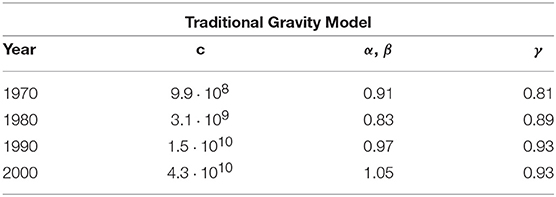
Table 1. Parameter values for the traditional Gravity Model used in Figure 1 and calculated by fitting Equation (1) (with the symmetry constraint α ≡ β) to all non-zero empirical bilateral trade flows via an Ordinary Least Square (OLS) regression of log-transformed weights.

FIGURE 1

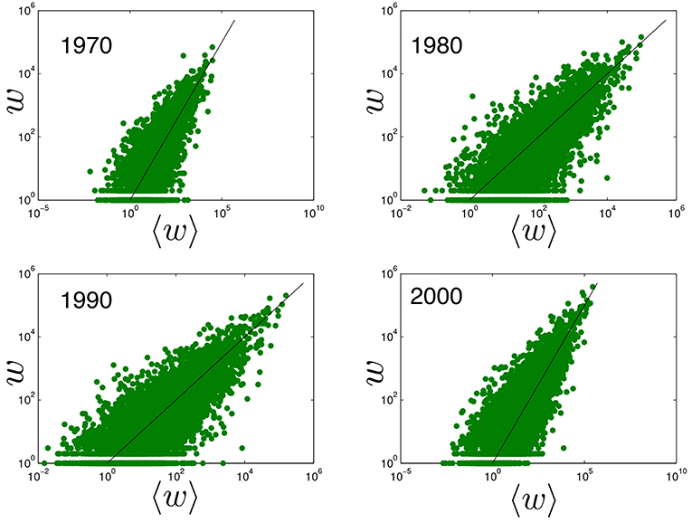
Figure 1. Empirical non-zero trade flows vs. the corresponding expectation under the traditional Gravity Model. Log-log plot comparing the empirical volume (y-axis) of all non-zero bilateral trade flows in the ITN with the corresponding expected volume (x-axis) predicted by the Gravity Model defined in Equation (1), with parameters estimated as reported in Table 1. Top left: year 1970, top right: year 1980, bottom left: year 1990, bottom right: year 2000. The black line is the identity line corresponding to the ideal, perfect match that would be achieved if the empirical weights were exactly equal to their expected values, i.e., in complete absence of randomness.

A related but more fundamental limitation of the GM is that, at least in its simplest and most natural implementations, it cannot generate zero volumes, thereby predicting a fully connected network [22–24]. This means that the GM can be fitted only to the non-zero weights, i.e., the volumes existing between pairs of connected countries. If used in this way, the model effectively disregards the empirical structure of the network, both as input (thus making predictions on the basis of incomplete data) and as output (thus failing to reproduce the topology). Operatively, the GM can be used only after the presence of a trade link has been established independently [22]. As observed in Linders and de Groot [21], “Omitting zero-flow observations implies that we lose information on the causes of (very) low trade,” because any fit to positive-only flows would significantly underestimate the effects of factors that diminish trade. This problem is particularly critical since roughly half of the possible links are found not to be realized in the real ITN [25–28]. Clearly, the same problem holds for the RM and any more general model of the form specified in Equation (2).

While there are variants and extensions of the GM that do generate zero weights and a realistic link density (e.g., the so-called Poisson pseudo-maximum likelihood models [20] and “zero-inflated” gravity models [21]), these variants systematically fail in reproducing the observed topology [10, 22]. In other words, while these models can generate the correct number of connections, they tend to put many of the latter in the “wrong place” in the network. Indeed, even in its generalized forms, the GM predicts a largely homogeneous network structure, while the empirical topology of the ITN is much more heterogeneous and complex [22, 23]. Established empirical signatures of this heterogeneity include a broad distribution of the degree (number of connections) and the strength (total trade volume) of countries [25–35], the rich-club phenomenon (whereby well-connected countries are also connected to each other) [36, 37], strong clustering and (dis)assortative patterns [26, 27]. These highly skewed structural properties are remarkably stable over time. However, they are not replicated by any current version of the GM [22].

2.2. Network Models of Trade

As we mentioned at the beginning, many processes of great economic relevance crucially depend on the large-scale topology of the ITN. In light of this result, the sharp contrast between the observed topological complexity of the ITN and the homogeneity of the network structure generated by the GM (including its extensions) call for major improvements in the modeling approach. In particular, in assessing the performance of a model of the ITN, emphasis should be put on how reliably the (global) empirical network structure, besides the (local) volume of trade, is replicated. In the network science literature, successful models of the ITN have been derived from the Maximum Entropy Principle [24–28, 38–44]. These models construct ensembles of random networks that have some desired topological property (taken as input from empirical data) and are maximally random otherwise. Typically, the constrained properties are chosen to be the degrees and/or the strengths of all nodes. In this way the models can perfectly replicate the observed strong heterogeneity of these purely local properties, and at the same time illustrate its immediate (i.e., prior to invoking any other more complicated network formation mechanism) structural effects on any higher-order topological property of the network. In the different context of financial networks, where the main challenge is a reliable inference of the unobserved topology of a network (typically of interconnected firms or banks) starting from partial, node-aggregate information [45], maximum-entropy models have recently turned out to deliver the best-performing reconstruction methods so far [43–45].

In general, different choices of the constrained properties lead to different degrees of agreement between the model and the data. This can generate intriguing and counter-intuitive insight about the structure of the ITN. For instance, contrary to what naive economic reasoning would predict, it turns out that the knowledge of purely binary local properties (e.g., node degrees) can be more informative than the knowledge of the corresponding weighted properties (e.g., node strengths). Indeed, while the binary network reconstructed only from the knowledge of the degrees of all countries is found to be topologically very similar to the real ITN, the weighted network reconstructed only from the strengths of all countries is found to be much denser and very different from the real network [26–28]. This is somewhat surprising, given that the economic literature largely postulates that weighted properties are per se more informative than the corresponding binary ones.

The solution to this apparent paradox lies in the fact that, while the knowledge of the entire weighted network is necessarily more informative than that of its binary projection (in accordance with economic postulates), the knowledge of certain marginal properties of the weighted network can be unexpectedly less informative than the knowledge of the corresponding marginal properties of the binary network. In fact, it turns out that if the degrees of countries are (not) specified in addition to the strengths of countries, the resulting maximum-entropy model can(not) reproduce the empirical weighted network of international trade satisfactorily [27, 40, 41].

An important take-home message is that, in contrast with the mainstream literature, models of the ITN should aim at reproducing not only the strength of countries (as the GM automatically does by approximately reproducing all non-zero weights), but also their degree (i.e., the number of trade partners) [26–28, 41]. In addition to these studies, an alternative approach, the Linear Gravity Transportation Model (LGTM), has also demonstrated the importance of the ITN topology [46]. In this model the monetary flow is balanced for each country (node) based on the number of trade partners (degree). The model produces expectations of the GDP of countries that are consistent with real data, using both the volume of trade flows and the topology of ITN as input. These studies indicate that, in order to devise improved models of the ITN, one should include the degrees, which are purely topological properties, among the main target quantities to replicate. This is the guideline we will follow in this paper.

Unlike the GM, maximum-entropy models of trade are a priori non-explanatory, i.e., they take as input structural properties (as opposed to explanatory economic factors) to explain other structural properties. However, they can in fact be used to select a posteriori an explicit, empirically validated functional dependence of the structure of the ITN on underlying explanatory factors. For models with country-specific constraints, this operation can be carried out as follows. Mathematically, controlling for node-specific properties is realized by assigning one or more Lagrange multipliers, also known as “hidden variables” or “fitness parameters” ${\overrightarrow{x}}_i$, to each node. If a certain choice of local constraints is found to replicate the higher-order properties of the real-world network satisfactorily, then one can look for an empirical relationship between the values of the associated hidden variables and those of candidate non-topological, country-specific factors of the type ${\overrightarrow{n}}_i$, like the GDP or total import/export. If the hidden variables are indeed (at least approximately) found to be functions of some country-specific factors [i.e., if ${\overrightarrow{x}}_i\approx \overrightarrow{f}({\overrightarrow{n}}_i)$], then one can replace ${\overrightarrow{x}}_i$ with $\overrightarrow{f}({\overrightarrow{n}}_i)$ in the maximum-entropy model, thus reformulating the latter as a model with explanatory variables (i.e., “regressors”) of trade, precisely like the GM. Already in one of the earliest studies on the ITN topology [30], the approach outlined above led to the definition of a GDP-driven model for the binary structure of the network, where ${\overrightarrow{x}}_i\propto {\mathrm{\text{GDP}}}_i$ (i.e., in this case ${\overrightarrow{x}}_i$ is taken to be one-dimensional). The model, which is a reformulation of a maximum-entropy model for binary networks with given degrees, predicts that the probability of a trade connection existing from country i to country j is

$\begin{array}{ll}{p}_{ij}=\frac{\delta {\mathrm{\text{GDP}}}_i{\mathrm{\text{GDP}}}_j}{1+\delta {\mathrm{\text{GDP}}}_i{\mathrm{\text{GDP}}}_j}\delta >0,& (3)\end{array}$

where δ is a free parameter that allows to reproduce the empirical link density. The model has been tested successfully in multiple ways [24, 25, 30, 32, 38].

The GM in Equation (1) and the maximum-entropy model in Equation (3) have complementary strengths and weaknesses, the former being a good model for non-zero volumes (while being a bad model for the topology) and the latter being a good model for the topology (while providing no information about trade volumes). An attempt to reconcile these two complementary and currently incompatible approaches has been recently proposed via the definition of an extension of the maximum-entropy model to the case of weighted networks [42]. Since, as we mentioned, a maximum-entropy model of weighted networks with given strengths and degrees [40] can correctly replicate many structural properties of the ITN [41], it makes sense to reformulate such a model as an economically inspired model of the ITN. Indeed, like in the binary case, the hidden variables enforcing the constraints are found to be strongly correlated with the GDP, thus allowing to express both p_ij and 〈w_ij〉 as functions of the GDP [42]. The resulting model is confirmed to be in good accordance with both the topology and the volumes observed in the real ITN.

Unfortunately, in the above approach the choice of country-specific constraints (degrees and strengths) only allows for regressors that have a corresponding country-specific nature. This makes the model in Almog et al. [42] incompatible with the inclusion of dyadic variables of the type ${\overrightarrow{D}}_{ij}$ and represents a strong limitation for (at least) two reasons. Firstly, one of the main lessons learned from the traditional GM is that the addition of geographic distances improves the fit to the empirical volumes significantly. Indeed, in light of the large body of knowledge accumulated in the international economics literature, it is hard to imagine a realistic and economically meaningful model of international trade that does not allow for simple pair-wise quantities controlling for trade costs and incentives, including geography [9, 10]. Secondly, even if the structure of the ITN can be replicated satisfactorily in terms of the “GDP-only” model defined in Equation (3) [25, 30, 32], recent analyses have found evidence that certain metric (although not necessarily geographic²) distances do also play a role in determining the topology of the ITN [47]. Together, these two pieces of evidence call for an inclusion of dyadic factors in 〈w_ij〉 and p_ij, and highlight a limitation of current maximum-entropy models based only on country-specific constraints.

Combining all the above considerations, it is clear that an improved model of the ITN should aim at retaining the realistic trade volumes postulated by models based on Equation (2) (including the GM, the RM, and possibly many more), while combining them with a realistic network topology generated by (extensions of) maximum-entropy models. Such a model should also aim at providing the full probability distribution, and not only the expected values as in Equation (1), of trade flows and, unlike the GDP-only model in Equation (3) [25] or its current weighted extension [42], allow for the inclusion of both dyadic and node-specific macroeconomic factors.

3. The Enhanced Gravity Model of International Trade

In this section, we introduce what we call the Enhanced Gravity Model (EGM) of trade. The EGM mathematically formalizes the two ingredients that, in light of the previous discussion, any “good” model of economic networks should feature: namely, realistic (trade) volumes and a realistic topology, both controllable by macroeconomic factors.

3.1. A Single Model for Topology and Weights

The first lesson we have learned is that Equation (2) is successful in reproducing link weights only after the existence of the links themselves has been preliminarly established. This implies that Equation (2), as a model of real-world trade flows, is actually unsatisfactory and should rather be reformulated as a conditional expectation of the weight w_ij, given that w_ij > 0. In other words, if a_ij denotes the entry of the adjacency matrix A = Θ(W) of the ITN (defined via the step function as a_ij = Θ(w_ij), i.e., a_ij = 1 if w_ij > 0 and a_ij = 0 if w_ij = 0), an improved model should be such that Equation (2) is replaced by

$\begin{array}{ll}\langle w_{ij}|a_{ij}=1\rangle =F_{\overrightarrow{\varphi }}({\overrightarrow{n}}_i,{\overrightarrow{n}}_j,{\overrightarrow{D}}_{ij})F>0,& (4)\end{array}$

where 〈w_ij|a_ij = 1〉 is the conditional expected weight of the trade link from country i to country j, given that such link exists. This operation ensures that, whatever the new model looks like, its predictions for the expected trade volume between connected pairs of countries remain identical to the ones proposed in more traditional macroeconomic models. For instance, choosing $F_{\overrightarrow{\varphi }}({\overrightarrow{n}}_i,{\overrightarrow{n}}_j,{\overrightarrow{D}}_{ij})=c{\mathrm{\text{GDP}}}_i^{\alpha }{\mathrm{\text{GDP}}}_j^{\beta }{R}_{ij}^{-\gamma }$ as in Equation (1) allows us to retain (in almost intact form) all the empirical knowledge that has accumulated in the econometrics literature since Jan Tinbergen's introduction of the GM. An important difference, however, is that in our model the trade volumes will be drawn from a different probability distribution.

The second lesson we have learned is that, in analogy with Equation (4), Equation (3) should be generalized to allow for both dyadic (${\overrightarrow{D}}_{ij}$) and node-specific (${\overrightarrow{n}}_i$) factors as follows:

$\begin{array}{ll}{p}_{ij}=\langle a_{ij}\rangle =\frac{G_{\overrightarrow{\psi }}({\overrightarrow{n}}_i,{\overrightarrow{n}}_j,{\overrightarrow{D}}_{ij})}{1+G_{\overrightarrow{\psi }}({\overrightarrow{n}}_i,{\overrightarrow{n}}_j,{\overrightarrow{D}}_{ij})}G>0,& (5)\end{array}$

where a crucial requirement is that G can in general be different from F in Equation (4) and, correspondingly, the vector $\overrightarrow{\psi }$ of parameters can be different from $\overrightarrow{\varphi }$. Note that, since p_ij is monotonic in G, the above expression is entirely general, i.e., we have put no restriction on the functional form of p_ij. It is also worth noticing that the explanatory factors used in Equations (4) and (5) need not coincide. However, to avoid using different symbols for the arguments of the two functions, we adopt the convention that ${\overrightarrow{D}}_{ij}$ and ${\overrightarrow{n}}_i$ denote the sets of all factors used as arguments of either F or G, and that these functions can have flat (i.e., no) dependence on some of their arguments. For instance, Equation (5) reduces to Equation (3) by setting ${\overrightarrow{n}}_i={\mathrm{\text{GDP}}}_i$ and assuming flat dependence on ${\overrightarrow{D}}_{ij}$, or it reduces to the hyperbolic model in García-Pérez et al. [47] by setting ${\overrightarrow{D}}_{ij}$ equal to the hyperbolic distance and assuming flat dependence on ${\overrightarrow{n}}_i$.

We want our model to produce both Equation (4) as the desired (gravity-like) conditional expectation for link weights and Equation (5) as a realistic expected topology. To do so, we introduce the full probability P(W) that the model produces a weighted network specified by the N × N matrix W with entries (w_ij). We are free to choose whether w_ij takes non-negative integer values [in which case P(W) is a multivariate Probability Mass Function, or PMF] or non-negative real values [in which case P(W) is a multivariate Probability Density Function, or PDF]. The distribution P(W) is the key quantity that fully specifies the model and determines both the topology and the link weights of the ITN. From P(W), focusing on a single pair i, j of nodes and integrating out all other pairs, we can define the dyadic distribution q_ij(w) indicating the probability (mass or density) that w_ij takes the particular value w. Note that the event w_ij > 0 indicates the presence of a trade link (i.e., a_ij = 1). By contrast, the event w_ij = 0 indicates the absence of a trade link (i.e., a_ij = 0) and is also included as a possible outcome in q_ij(w). The normalization condition is therefore $\sum _{w\ge 0}{q}_{ij}(w)=1$ (for integer weights) or ${\int }_{w\ge 0}dw{q}_{ij}(w)=1$ (for continuous weights, in which case we anticipate that q_ij(w) will have a delta-like point mass at w = 0) for all i, j. Note that we are not assuming independence of the trade volumes w_ij and w_kl between two distinct country pairs, or equivalently the factorization of P(W) into the product ∏_i,jq_ij(w_ij) of dyadic probabilities. However, we will later find that the desired model has precisely this independence property. Importantly, unlike in the traditional GM, in our approach dyadic independence is a consequence and not a postulate.

We now look for the form of q_ij(w) that enforces both Equations (4) and (5). Let us consider the latter first. In terms of q_ij(w), the probability p_ij that i and j are connected (irrespective of the volume of trade) is given by the complement of the probability q_ij(0) that they are not connected, i.e.,

$\begin{array}{ll}{p}_{ij}=1-q_{ij}(0)=\{\begin{array}{ll}{\displaystyle {\sum }_{w>0}{q}_{ij}}(w) \hfill & (\text{integer})\hfill \\ {\displaystyle {\int }_{w>0}{q}_{ij}}(w) dw \hfill & (\text{real})\hfill \end{array}& (6)\end{array}$

where, for real-valued weights, q_ij(0) denotes the point mass, i.e., the magnitude of the delta-like probability density function q_ij(w), at w = 0. Imposing that Equation (6) has the form dictated by Equation (5) leads to the following unique choice for q_ij(0):

$\begin{array}{ll}{q}_{ij}(0)=\frac{1}{1+G_{\overrightarrow{\psi }}({\overrightarrow{n}}_i,{\overrightarrow{n}}_j,{\overrightarrow{D}}_{ij})}G>0.& (7)\end{array}$

We now relate q_ij(w) to Equation (4) in a similar manner. The expected trade volume, irrespective of whether a link exists, is

$\begin{array}{ll}\langle w_{ij}\rangle \equiv \{\begin{array}{ll}{\displaystyle {\sum }_{w>0}{q}_{ij}}(w)\hfill & (\text{integer})\hfill \\ {\displaystyle {\int }_{w>0}w} q_{ij}(w) dw \hfill & (\text{real})\hfill \end{array}& (8)\end{array}$

(note that the event w = 0 does not contribute to the above quantity). On the other hand the conditional probability that w_ij equals w, given that the link is realized (w > 0), is

$\begin{array}{ll}{q}_{ij}(w|a_{ij}=1)=\{\begin{array}{ll}\frac{q_{ij}(w)}{p_{ij}}\hfill & w>0\hfill \\ 0\hfill & w=0\hfill \end{array}& (9)\end{array}$

and its expected value gives the conditional expectation of the link weight, given that the link exists:

$\begin{array}{ll}\langle w_{ij}|a_{ij}=1\rangle =\frac{\langle w_{ij}\rangle }{p_{ij}}.& (10)\end{array}$

Setting Equation (10) equal to Equation (4) leads to

$\begin{array}{ll}\langle w_{ij}\rangle =\frac{F_{\overrightarrow{\varphi }}({\overrightarrow{n}}_i,{\overrightarrow{n}}_j,{\overrightarrow{D}}_{ij})G_{\overrightarrow{\psi }}({\overrightarrow{n}}_i,{\overrightarrow{n}}_j,{\overrightarrow{D}}_{ij})}{1+G_{\overrightarrow{\psi }}({\overrightarrow{n}}_i,{\overrightarrow{n}}_j,{\overrightarrow{D}}_{ij})}F,G>0.& (11)\end{array}$

Equation (11) carries an important message. It reveals that, while a superficial inspection of Equation (8) might suggest that the expected trade volume 〈w_ij〉 is independent of the topology of the ITN, i.e., on q_ij(0) or equivalently G, this is actually not the case. In fact, q_ij(0) is coupled to the other values q_ij(w) (with w > 0) through the normalization condition manifest in Equation (6). This necessarily implies that the topology of the ITN must have an immediate effect on the expected volume of trade between any two countries. This effect is rigorously quantified in Equation (11), which shows that 〈w_ij〉 depends on both F and G. This result confirms the inconsistency of the traditional GM defined in terms of Equation (1) and of any of its extensions of the form given by Equation (2). By contrast, the expected topology of the ITN is independent of the expected volumes of trade, since p_ij depends on G but not on F. This simple but, to the best of our knowledge, previously unrecognized result highlights a nontrivial asymmetry between weights and topology in the ITN and, by extension, in any (economic) network described by our generic expressions involving F and G. This basic finding provides a natural explanation for the aforementioned empirical observation that the topology of the ITN and several other networks can be satisfactorily reconstructed from aggregate local constraints [26, 40], while the same result does not hold for the weighted structure of the same network(s) [27, 28], unless topological information is explicitly included as an additional constraint [40, 41].

3.2. Maximum Entropy Construction

Equations (7) and (11) fix two important properties we require for q_ij(w) and ultimately P(W), but they do not specify these probability distributions uniquely. To do so, we invoke the Maximum-Entropy Principle to ensure that the functional form of P(W) is maximally random, given the desired constraints. As is well known, this procedure is guaranteed to lead to the least biased inference, i.e., to introduce no unjustified “hidden” assumption in picking a specific form of P(W) [43, 44]. In applying this method we will focus primarily on the case of integer-valued link weights, since this requirement matches the datasets in our analysis. The case of real-valued link weights is treated in the Appendix and the corresponding key results are briefly reported at the end of this section.

We look for the form of P(W) that maximizes the entropy functional

$\begin{array}{ll}S\left[P\right]=-{\displaystyle \sum _{\text{W}}}P(\text{W})lnP(\text{W})& (12)\end{array}$

(where the sum extends over all weighted graphs with N nodes, non-negative integer link weights, and such that w_ii = 0 for all i) subject to the constraints specified by Equations (7) and (11). Since Equation (7) is equivalent to Equation (5), we select 〈a_ij〉 and 〈w_ij〉 (for all pairs i ≠ j) as the two sets of constraints specifying our model. In this way, if we introduce α_ij and β_ij as the (real-valued) Lagrange multipliers required to enforce the expected value of a_ij = Θ(w_ij) and w_ij respectively [where Θ(x) = 1 if x > 0 and Θ(x) = 0 otherwise], then the maximum-entropy problem becomes equivalent to one solved exactly in Garlaschelli and Loffredo [48]. There, it was shown that upon introducing the so-called Hamiltonian

$\begin{array}{ll}H(W)={\displaystyle {{\displaystyle \sum }}^{}_{i,j}}\left[{\alpha }_{ij}\Theta (w_{ij})+{\beta }_{ij}{w}_{ij}\right],& (13)\end{array}$

(representing a linear combination of the quantities whose expected value is being constrained) and the partition function $Z=\sum _{\text{W}}{e}^{-H(\text{W})}$, the maximum-entropy probability P*(W) with constraints 〈a_ij〉 and 〈w_ij〉 is found to be

$\begin{array}{ll}{P}^{*}(\text{W})=\frac{e^{-H(\text{W})}}{Z}={\displaystyle \prod _{i,j}}{q}_{ij}^{*}(w_{ij}),& (14)\end{array}$

where, given $x_{ij}\equiv e^{-{\alpha }_{ij}}\in (0,+\infty )$ and $y_{ij}\equiv e^{-{\beta }_{ij}}\in (0,1)$,

$\begin{array}{ll}{q}_{ij}^{*}(w)\equiv \frac{x_{ij}^{\Theta (w)}{y}_{ij}^w(1-y_{ij})}{1-y_{ij}+x_{ij}{y}_{ij}},w\ge 0& (15)\end{array}$

is the resulting (maximum-entropy) probability that the link from node i to node j carries a weight w. This probability is called the Bose-Fermi distribution, as it unifies the Bose-Einstein and Fermi-Dirac distributions encountered in quantum statistical physics [48]. We stress again that all our formulas apply to both directed and undirected representations of the network and, correspondingly, the sums and products over i, j should be interpreted as i ≠ j in the directed case (where the pairs i, j and j, i are different) and as i < j in the undirected one (where the pair i, j is the same as the pair j, i). As we had anticipated, the factorization of P*(W) in terms of products of $q_{ij}^{*}(w)$ shows that, for this particular choice of the constraints, pairs of nodes turn out to be statistically independent as in the standard GM approach, even if we have not assumed this independence as a postulate in our approach.

Importantly, while the constraints used in the maximum-entropy models of the ITN considered so far in the literature are observed topological properties (e.g., the degrees and/or the strengths of nodes), the constraints considered here are economically-driven expectations, namely Equations (5) and (11). This key step allows us to reconcile macroeconomic and network approaches within a generalized framework and represents an important difference with respect to previous models. In particular, we use Equations (6), (8) and (10) to express p_ij, 〈w_ij〉 and 〈w_ij|a_ij = 1〉 in terms of x_ij and y_ij [48]:

$\begin{array}{ll}{p}_{ij}=1-q_{ij}^{*}(0)=\frac{x_{ij}{y}_{ij}}{1-y_{ij}+x_{ij}{y}_{ij}},& (16)\end{array}$

$\begin{array}{ll}\langle w_{ij}\rangle ={\displaystyle \sum _{w>0}}w{q}_{ij}^{*}(w)=\frac{p_{ij}}{1-y_{ij}},& (17)\end{array}$

$\begin{array}{ll}\langle w_{ij}|a_{ij}=1\rangle =\frac{\langle w_{ij}\rangle }{p_{ij}}=\frac{1}{1-y_{ij}}.& (18)\end{array}$

The above expressions allow us to rewrite Equation (15) as

$\begin{array}{ll}{q}_{ij}^{*}(w)=\{\begin{array}{ll}1-p_{ij}\hfill & w=0,\hfill \\ p_{ij} y_{ij}^{w-1}(1-y_{ij}) \hfill & w>0.\hfill \end{array}& (19)\end{array}$

Now, equating Equation (16) to Equation (5) and Equation (17) to Equation (11) [or, equivalently, Equation (18) to Equation (4)] allows us to find the values of x_ij and y_ij solving the original problem:

$\begin{array}{ll}{x}_{ij}=\frac{G_{\overrightarrow{\psi }}({\overrightarrow{n}}_i,{\overrightarrow{n}}_j,{\overrightarrow{D}}_{ij})}{F_{\overrightarrow{\varphi }}({\overrightarrow{n}}_i,{\overrightarrow{n}}_j,{\overrightarrow{D}}_{ij})-1},& (20)\end{array}$

$\begin{array}{ll}{y}_{ij}=\frac{F_{\overrightarrow{\varphi }}({\overrightarrow{n}}_i,{\overrightarrow{n}}_j,{\overrightarrow{D}}_{ij})-1}{F_{\overrightarrow{\varphi }}({\overrightarrow{n}}_i,{\overrightarrow{n}}_j,{\overrightarrow{D}}_{ij})}.& (21)\end{array}$

Inserting Equations (20) and (21) into Equation (19), we finally get the explicit probability $q_{ij}^{*}(w)$ of any two countries trading a volume w, as a function of any choice of the factors ${\overrightarrow{n}}_i$ and ${\overrightarrow{D}}_{ij}$. In terms of conditional probabilities, the model becomes extremely simple: establishing a link from country i to country j is a Bernoulli trial with success probability p_ij given by Equation (5); if realized, this link acquires a weight w with probability

$\begin{array}{ll}{q}_{ij}^{*}(w|a_{ij}=1)=\{\begin{array}{ll}0\hfill & w=0,\hfill \\ \frac{{\left[F_{\overrightarrow{\varphi }}({\overrightarrow{n}}_i,{\overrightarrow{n}}_j,{\overrightarrow{D}}_{ij})-1\right]}^{w-1}}{{\left[F_{\overrightarrow{\varphi }}({\overrightarrow{n}}_i,{\overrightarrow{n}}_j,{\overrightarrow{D}}_{ij})\right]}^w}\hfill & w>0,\hfill \end{array}& (22)\end{array}$

which is a geometric distribution representing the chance of w−1 consecutive successes, each with probability y_ij, followed by a failure with probability 1−y_ij. The above result provides an insightful interpretation of the realized volumes in the model in terms of processes of link establishment and link reinforcement (see section 5).

3.3. Maximum-Likelihood Parameter Estimation

We now take an econometric perspective and discuss how the model parameters can be chosen to optimally fit a specific empirical instance of the network. To this end, we use the Maximum Likelihood (ML) principle applied to network models [38]. If W* denotes the weight matrix (with entries $w_{ij}^{*}$) of the empirical network, our model generates this particular matrix with probability P*(W*). We therefore define the log-likelihood function as

$\begin{array}{l}ℒ(\overrightarrow{\varphi },\overrightarrow{\psi })=\ln P^{*}(W^{*})={\displaystyle \sum _{i,j}\ln \frac{{\left(G_{\overrightarrow{\psi }}\right)}^{a_{ij}^{*}}{\left(F_{\overrightarrow{\varphi }}-1\right)}^{w_{ij}^{*}-a_{ij}^{*}}}{\left(1+G_{\overrightarrow{\psi }}\right){\left(F_{\overrightarrow{\varphi }}\right)}^{w_{ij}^{*}}}}\end{array}$

(where we have dropped the dependence of F and G on ${\overrightarrow{n}}_i$, ${\overrightarrow{n}}_j$, ${\overrightarrow{D}}_{ij}$) and look for the parameter values ${\overrightarrow{\varphi }}^{*},{\overrightarrow{\psi }}^{*}$ that maximize ${L}(\overrightarrow{\varphi },\overrightarrow{\psi })$ by requiring that all the first derivatives with respect to $\overrightarrow{\varphi }$ and $\overrightarrow{\psi }$ vanish simultaneously:

$\begin{array}{ll}{\overrightarrow{\nabla }}_{\overrightarrow{\varphi }}{L}(\overrightarrow{\varphi },\overrightarrow{\psi })={\displaystyle \sum _{i,j}}\left[\frac{w_{ij}^{*}-a_{ij}^{*}}{F_{\overrightarrow{\varphi }}-1}-\frac{w_{ij}^{*}}{F_{\overrightarrow{\varphi }}}\right]{\overrightarrow{\nabla }}_{\overrightarrow{\varphi }}{F}_{\overrightarrow{\varphi }}=\overrightarrow{0}& (23)\end{array}$

$\begin{array}{ll}{\overrightarrow{\nabla }}_{\overrightarrow{\psi }}{L}(\overrightarrow{\varphi },\overrightarrow{\psi })={\displaystyle \sum _{i,j}}\left[\frac{a_{ij}^{*}}{G_{\overrightarrow{\psi }}}-\frac{1}{1+G_{\overrightarrow{\psi }}}\right]{\overrightarrow{\nabla }}_{\overrightarrow{\psi }}{G}_{\overrightarrow{\psi }}=\overrightarrow{0}.& (24)\end{array}$

For probability distributions belonging to the exponential family, i.e., in the form given by Equation (14) like the one we are considering, the second derivatives of the log-likelihood coincide with (minus) the covariances between the constraints included in the Hamiltonian defined in Equation (13) (see for instance [49, 50]). Since covariance matrices are positive-semidefinite (and actually positive-definite if the chosen constraints are linearly independent, i.e., non-redundant), ${L}({\overrightarrow{\varphi }}^{*},{\overrightarrow{\psi }}^{*})$ is indeed a (global, in the positive-definite case) maximum for ${L}(\overrightarrow{\varphi },\overrightarrow{\psi })$, ensuring that the solution $({\overrightarrow{\varphi }}^{*},{\overrightarrow{\psi }}^{*})$ to Equations (23) and (24) yields the optimal parameter values in our model. Selecting these values into Equations (20) and (21) yields the values $x_{ij}^{*}$ and $y_{ij}^{*}$ that, when inserted into Equation (15), fully specify the model.

The above expressions, which are valid for any specification of the EGM, show that the estimation of the parameter $\overrightarrow{\varphi }$ nicely separates from that of $\overrightarrow{\psi }$. This result solves, in a single step, two major problems encountered in previous econometric approaches: on one hand, in most alternative models the estimation of the parameters determining the expected weights is badly affected by the presence of the zeroes; on the other hand, the expected number of zeroes may paradoxically depend on the (arbitrary) units of measure for the weights. For instance, if q_ij(w) is a Poisson distribution as in zero-inflated GMs [20–22], then its only parameter (the mean) determines both the magnitude of link weights and the connection probability p_ij. As the monetary units in the data are changed arbitrarily (e.g., from dollars to thousands of dollars), so will the estimated mean and the resulting expected number of zeroes. By contrast, in our model the monetary units affect ${\overrightarrow{\varphi }}^{*}$ but not ${\overrightarrow{\psi }}^{*}$ (hence F as they should, but not G).

3.4. Real-Valued Trade Flows

The above results can be adapted in a straightforward, although more technical, fashion to the case when link weights are assumed to take non-negative real values. The entire derivation is reported in the Appendix. For brevity, here we only report the main results.

In the real-valued case, P*(W) is a multivariate PDF (rather than a PMF) and we look for its form by maximizing a modified version of the entropy functional S[P], under the same constraints on 〈a_ij〉 and 〈w_ij〉 (for all pairs i, j) used above and still given by Equations (5) and (11). The result is again of the factorized form given by Equation (14), where the Hamiltonian H(W) is still the one defined in Equation (14) while the partition function Z is different and the resulting expression for $q_{ij}^{*}(w)$ is

$\begin{array}{ll}{q}_{ij}^{*}(w)=\delta (w)(1-p_{ij})+\Theta (w)p_{ij}\frac{e^{-w/F_{\overrightarrow{\varphi }}({\overrightarrow{n}}_i,{\overrightarrow{n}}_j,{\overrightarrow{D}}_{ij})}}{F_{\overrightarrow{\varphi }}({\overrightarrow{n}}_i,{\overrightarrow{n}}_j,{\overrightarrow{D}}_{ij})},& (25)\end{array}$

where δ(w) is the Dirac delta function and p_ij is still given by Equation (5).

The above expression shows that $q_{ij}^{*}(w)$ has now a point mass of magnitude 1−p_ij at w = 0, followed by a purely exponential probability density for w > 0. By design, the above PDF still produces the desired conditional expected trade volume 〈w_ij|a_ij = 1〉, connection probability p_ij and unconditional expected trade volume 〈w_ij〉 given by Equations (4), (5) and (11) respectively. Establishing a link from country i to country j is still a Bernoulli trial with success probability p_ij given by Equation (5); if realized, this link acquires a weight w with conditional probability density

$\begin{array}{ll}{q}_{ij}^{*}(w|a_{ij}=1)=\{\begin{array}{ll}0\hfill & w=0,\hfill \\ \frac{e^{-w/F_{\overrightarrow{\varphi }}({\overrightarrow{n}}_i,{\overrightarrow{n}}_j,{\overrightarrow{D}}_{ij})}}{F_{\overrightarrow{\varphi }}({\overrightarrow{n}}_i,{\overrightarrow{n}}_j,{\overrightarrow{D}}_{ij})}\hfill & w>0,\hfill \end{array}& (26)\end{array}$

which is now a purely exponential distribution with the desired (conditional) mean $F_{\overrightarrow{\varphi }}({\overrightarrow{n}}_i,{\overrightarrow{n}}_j,{\overrightarrow{D}}_{ij})$.

The estimation of the parameters $\overrightarrow{\varphi }$ and $\overrightarrow{\psi }$ can be carried out using the ML principle via a straightforward recalculation of the log-likelihood ${L}(\overrightarrow{\varphi },\overrightarrow{\psi })=ln{P}^{*}({\text{W}}^{*})$ and a corresponding adaptation of Equations (23) and (24).

4. Empirical Analysis

We can finally test the predictions of our model against empirical international trade data. The datasets are described in the Appendix. Here, it suffices to report that trade volumes are reported in U.S. dollars and are therefore integer-valued. For this reason, throughout our analysis we will adopt the formulas we obtained assuming integer weights. Clearly, the same analysis can be easily repeated for real-valued volumes by using the corresponding formulas we have provided for real weights.

4.1. Model Specification

We adopt an undirected network description (where the connection between two countries carries a weight equal to the total trade in either direction) to facilitate the definition of the topological properties characterizing the ITN. Previous work has shown that, given the highly symmetric structure of the ITN, the undirected representation retains all the basic properties of the network [26, 27, 30].

We choose $F_{\overrightarrow{\varphi }}({\overrightarrow{n}}_i,{\overrightarrow{n}}_j,{\overrightarrow{D}}_{ij})$ in such a way that the expected non-zero trade flow 〈w_ij|a_ij = 1〉 is the same as in the GM defined by Equation (1) (now interpreted as a conditional expectation). This means choosing ${\overrightarrow{n}}_i={\mathrm{\text{GDP}}}_i$, ${\overrightarrow{D}}_{ij}=R_{ij}$, $\overrightarrow{\varphi }=(c,\alpha ,\gamma )$ and

$\begin{array}{ll}{F}_{\overrightarrow{\varphi }}({\overrightarrow{n}}_i,{\overrightarrow{n}}_j,{\overrightarrow{D}}_{ij})=c{({\mathrm{\text{GDP}}}_i{\mathrm{\text{GDP}}}_j)}^{\alpha }{R}_{ij}^{-\gamma },& (27)\end{array}$

where we have set β ≡ α due to undirectedness. Similarly, we choose $G_{\overrightarrow{\psi }}({\overrightarrow{n}}_i,{\overrightarrow{n}}_j,{\overrightarrow{D}}_{ij})$ in such a way that the probability p_ij is the same as in the model defined in Equation (3), i.e., $\overrightarrow{\psi }=\delta$ and

$\begin{array}{ll}{G}_{\overrightarrow{\psi }}({\overrightarrow{n}}_i,{\overrightarrow{n}}_j,{\overrightarrow{D}}_{ij})=\delta {\mathrm{\text{GDP}}}_i{\mathrm{\text{GDP}}}_j.& (28)\end{array}$

With the above specification, the expected topology does not depend on any dyadic factor. This is the simplest choice that is found to reproduce the topology of the ITN very well [25, 30, 32, 38] and is supported by empirical evidence that dyadic factors like geographic distances [51] and trade agreements [47] have a much weaker effect on the purely binary topology of the ITN than on trade volumes. Of course our formalism has been designed in such a way that we can immediately add dyadic factors and is therefore much more general. For instance, we might easily add “hidden” metric distances inferred via an optimal geometric embedding [47] (although they would not be identifiable with some empirically measurable, “external” macroeconomic factors like those used elsewhere in our model).

Given the above model specification, for a given instance W* of the empirical network we find the optimal parameter values c*, α*, γ* and δ* through the ML conditions given by Equations (23) and (24). Importantly, Equation (24) reads in this case $\partial {L}/\partial \delta =0$ and yields a value δ* that ensures that the expected number of links $\sum _{i,j}{p}_{ij}=\sum _{i,j}{G}_{\overrightarrow{\psi }}/(1+G_{\overrightarrow{\psi }})$ is exactly equal to the empirical number $L^{*}=\sum _{i,j}{a}_{ij}^{*}$, irrespective of the volumes of trade. This result, which is equivalent to what is found for the purely binary model defined by Equation (3) [38], shows that, unlike the standard GM, our model always generates the correct number of links and, unlike some more complicated variants of the GM, it does so independently of the monetary units chosen for the volumes.

4.2. Testing the Model Against Real Data

We first test the performance of the EGM in replicating the empirical trade volumes, i.e., the purely local (dyadic) structure of the ITN. In Figure 2, superimposed to the previous results for the standard GM given by Equation (1) and already shown in Figure 1, the empirical non-zero link weights $w_{ij}^{*}$ are also compared with their conditional expected value 〈w_ij|a_ij = 1〉 under the EGM given by Equation (27). As mentioned above, for the EGM the parameters are obtained via the ML principle as prescribed by Equation (23) and their resulting values are reported in Table 2. As expected, the sets of points generated by the two models largely overlap, confirming that, in terms of trade volumes, the EGM cannot do worse than the GM. Moreover, the EGM turns out to be more parsimonious than the GM as it achieves a narrower scatter of points while having no dedicated free parameter to tune the variance (as already mentioned, the GM usually assumes that each trade volume is drawn from a certain probability distribution, typically a normal or log-normal one, with mean value given by Equation (1) and variance specified by an additional free parameter).

TABLE 2

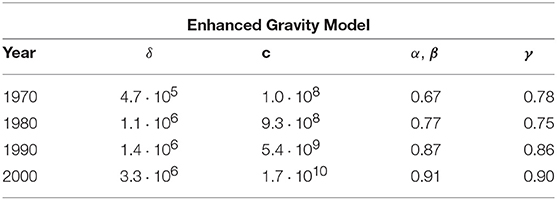
Table 2. Parameter values for the Enhanced Gravity Model calculated by considering integer link weights (equal to integer multiples of the monetary unit used in the dataset) and carrying out the corresponding ML estimation as prescribed by Equations (23) and (24).

FIGURE 2

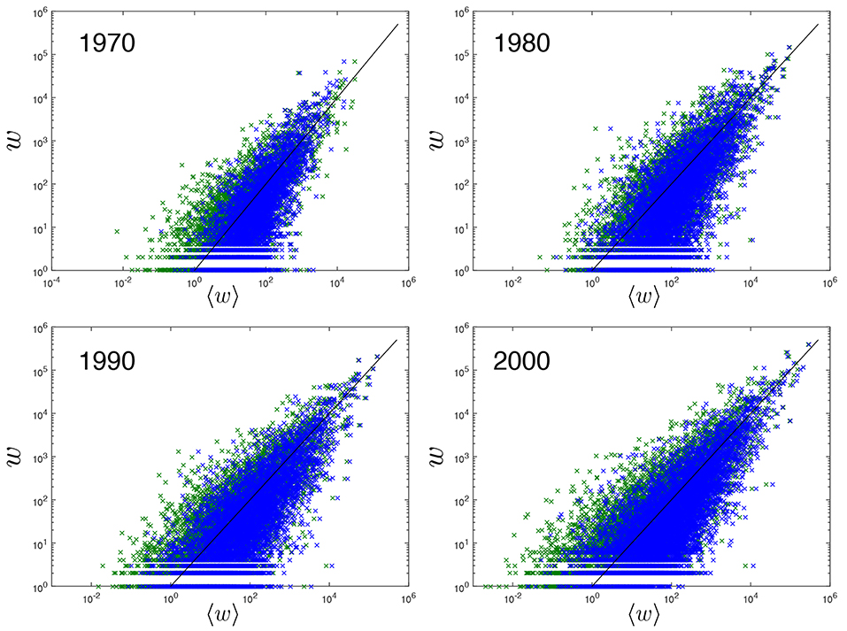
Figure 2. Empirical non-zero trade flows vs. the corresponding expectations under the traditional Gravity Model and the Enhanced Gravity Model. Log-log plot comparing the empirical volume (y-axis) of all non-zero bilateral trade flows in the ITN with the corresponding (conditional) expected volume (x-axis) predicted by the Gravity Model defined in Equation (1) (green, parameters estimated as reported in Table 1) and by the Enhanced Gravity Model defined in Equations (4) and (27) (blue, parameters estimated as reported in Table 2). Top left: year 1970, top right: year 1980, bottom left: year 1990, bottom right: year 2000. The black line is the identity line corresponding to the ideal, perfect match that would be achieved if the empirical weights were exactly equal to their (conditional) expected values, i.e., in complete absence of randomness.

Importantly, comparing the values of the parameters α, β, γ reported in Table 2 for the EGM with the corresponding values of the same parameters shown previously in Table 1 for the GM, we see that the GM yields systematically larger parameter values (especially so for α, β). This means that, with respect to the EGM, the GM overestimates the effects of both GDP and geographic distance, and this is especially true for the GDP. This is due to the fact that the EGM is used to explain not only the volume of realized trade flows, but also their existence, and has separate functions (F and G) with possibly overlapping sets of explanatory factors (GDP is the common element in this case) but in any case distinct sets of parameters (α, β, γ on one hand and δ on the other), to take these two aspects into account. The effects of GDP and distance captured by the parameters α, β, γ are only those conditional on a link being created, while discounting the effects of link creation itself via the parameter δ. Note that α, β, γ and δ are all found to be monotonically increasing over time by the EGM, highlighting a steady increase of the effects of GDP and distance (even if milder than observed in the GM) and of the density of connections. In fact, as the network density becomes higher (larger δ in the EGM), we see a smaller discrepancy between the fitted values of α, β in the two models, consistently with the idea that, if all pairs of countries were connected, then both the GM and the EGM would estimate the effects of GDP only through the lens of trade volumes, because the GDP would no longer explain the (fully connected) topology in such an extreme situation.

In order to better understand the differences between the trade volumes predicted by the two models, in Figure 3 we plot the cumulative distribution P_≥(w) counting the fraction of link weights larger than or equal to w in the empirical (red), GM-generated (green) and EGM-generated (blue) networks. All distributions are normalized as P_≥(0) = 1 in order to include zero weights, corresponding to pairs of countries that are not connected, in their support. Note that P_≥(w) is not simply the integral of $q_{ij}^{*}(w)$ because the latter is a probability distribution defined for a specific pair of countries, while the former is defined for the entire network and hence determined by the combination of all pair-specific probabilities. We see that the empirical distribution has a discontinuous jump at w = 1, as it drops from a value P_≥(1−ϵ) = 1 to a value P_≥(1 + ϵ) ≈ 0.53, where ϵ > 0 is arbitrarily small. Recalling that link weights take only non-negative integer values in our analysis, this discontinuity indicates that there are roughly 47% pairs of countries that are not connected (w = 0) in this particular snapshot of the ITN, so that the distribution keeps the value P_≥(w) = 1 for w ∈ [0, 1] and, as we cross the smallest allowed non-zero weight value (w = 1), it drops by a value 0.47 as it no longer “sees” those unconnected pairs. As bigger weights (w > 1) are considered, the distribution continues to decrease continuously all the way to P_≥(+∞) = 0, indicating that the only discontinuity we see at w = 1 is actually due to the excess probability mass at zero weights produced by the link-generating process. Remarkably, the empirical distribution is closely matched by the EGM. The fact that this model replicates both the location and size of the discontinuity indicates a correctly predicted number of missing trade connections in the ITN topology. By contrast, the GM predicts a fully connected network, evidenced from the absence of the discontinuity. Pairs of countries that are unconnected in the real ITN are unavoidably given a positive weight by the GM and hence misplaced to the right in the distribution, which results in exceedingly large values of the green curve with respect to the other two curves. We know that in the EGM the discontinuity is indeed due to the extra point mass at w = 0 in the expression of $q_{ij}^{*}(w)$ given by Equations (15) or (19). Note that, technically, one can speak of a “discontinuity” only if weights take continuous values. This would be possible by replicating our analysis in the case of real-valued weights using the results provided in the Appendix and summarized in Equation (25). Importantly, in this case the jump in P_≥(w) would be observed precisely at the “true” value w = 0, consistently with the genuine delta-like form of $q_{ij}^{*}(w)$ given by Equation (25) [only, it would no longer be possible to show the discontinuity of P_≥(w) along a logarithmic axis and plot the full cumulative distribution]. The EGM would again correctly match both location and size of the empirical discontinuity (since p_ij, hence the expected number of positive weights, is identical in the discrete and continuous versions of the model). For positive weights, the real-valued EGM would continuously interpolate the discrete points of the integer-valued EGM because this is a generic property of geometric and exponential distributions with the same expected value. So, in either specification, the EGM nicely replicates both the empirical distribution of strictly positive link weights and the sharp peak “jumping out” from it, while the GM does not.

FIGURE 3

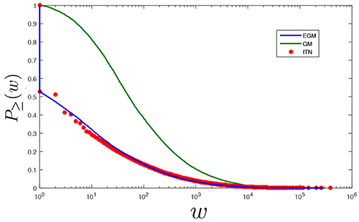
Figure 3. Empirical and model-generated cumulative distributions of trade flows. Log-linear plot comparing the empirical cumulative distribution of trade flows (normalized in order to include zero flows) in the ITN for the year 2000 (red) with the corresponding distributions obtained using the Gravity Model defined in Equation (1) (green, parameters estimated as reported in Table 1) and the Enhanced Gravity Model defined in Equations (4) and (27) (blue, parameters estimated as reported in Table 2). Note the discontinuous jump due to the ≈47% pairs of unconnected countries in both the empirical and the EGM-generated curves, and the absence of such a feature in the GM-generated curve (for which missing links are incorrectly given a positive weight).

We now want to check whether the trade links, besides being predicted in correct number by the EGM, are also placed between the correct pairs of countries by the same model. This means moving the focus of our analysis toward the purely binary, global topology of the ITN. As a first qualitative illustration setting the stage for this analysis, in Figure 4 we show all the trade links of the country with maximum degree (USA), the one with minimum degree (Western Sahara) and one with intermediate degree (Vanuatu). We also show the corresponding predictions under the standard GM (where Equation (1) is first fitted to the non-zero flows and then extended to all pairs of countries) and the EGM. The traditional GM predicts a fully connected network, i.e., an expected degree 〈_ki〉GM = N−1 for all i. This prediction may be accidentally correct for one or a few countries with maximal degree, if such countries turn out to be present in the network (in this case, this does not even happen as the maximum observed degree is k = 203 for USA), but deteriorates unavoidably and dramatically for other countries as their degree decreases. By contrast, the EGM gives an expected degree ${\langle k_i\rangle }_{EGM}=\sum _{j\ne i}{p}_{ij}$ (see Appendix) which is in good agreement with the empirical one for the entire range of connectivity.

FIGURE 4

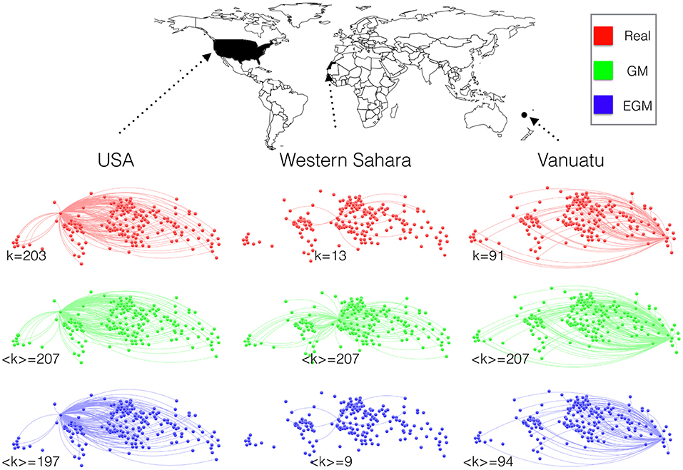
Figure 4. Country-based network configurations for year 2011 in the real ITN (red), the GM (green), and the EGM (blue). For three representative countries, we show the connections to all trade partners in the world. The total number of countries in the data (see Appendix) is N = 208. The three countries are selected on the basis of their empirical degree k: the country with maximum degree (USA, k = 203), the one with minimum degree (Western Sahara, k = 13), and one with intermediate degree (Vanuatu, k = 91). The GM produces always the maximum possible number (N−1) of connections. By contrast, the EGM produces connections randomly with probability p_ij, so links change from realization to realization. The expected degree is however independent of the individual realizations and is close to the empirical one for all countries. We have selected a typical realization that produces a degree equal to the expected degree for each of the three countries.

We now consider higher-order topological properties as a more stringent and quantitative test. In the top left panel of Figure 5 we plot the average degree ($k_i^{nn}$) of the trade partners of each country i vs. the number of such partners, i.e., the degree (k_i) of country i itself. Similarly, in the top right panel of Figure 5 we plot the clustering coefficient (c_i), i.e., the fraction of trade partners of country i that trade with each other, again vs. the number (k_i) of such partners. The empirical quantities are compared with the expected quantities under the GM and the EGM. The exact expressions for both empirical and expected quantities are provided in the Appendix. The decreasing empirical trends observed in both plots show that the trade partners of poorly connected countries (small k_i) are on average highly connected, both to the rest of the world (large $k_i^{nn}$) and among themselves (large c_i). By contrast, countries that trade with a high-degree country (large k_i) are on average poorly connected, both to the rest of the world (small $k_i^{nn}$) and among themselves (small c_i). For both properties, we find that the EGM is in excellent agreement with the empirical ITN, as opposed to the classical GM which systematically generates nearly constant and much higher values as a result of predicting a complete network.

FIGURE 5

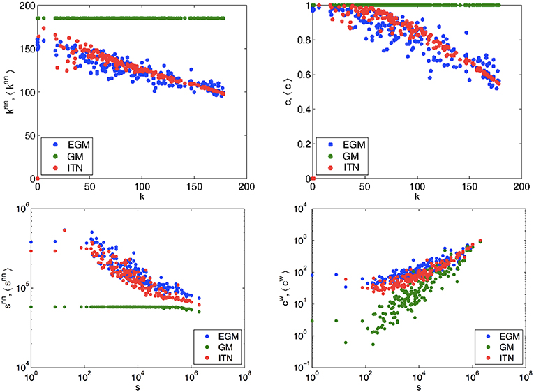
Figure 5. Network properties in the real ITN (red), the GM (green), and the EGM (blue). Top left: average nearest neighbor degree $k_i^{nn}$ vs. degree k_i for all nodes. Top right: clustering coefficient c_i vs. degree k_i for all nodes. Bottom left: average nearest neighbor strength $s_i^{nn}$ vs. strength s_i for all nodes. Bottom right: weighted clustering coefficient $c_i^w$ vs. strength s_i for all nodes. All results are for the snapshot of the ITN in the year 2000. For all the other years in the analyzed sample, we systematically obtained very similar results. See Appendix for information about the data and all definitions of empirical and observed quantities.

Having checked that the EGM does very well in separately replicating both the local link weights and the global topology of the ITN, we now perform a last and most severe test monitoring properties that combine topological and weighted information together (all definitions are again given in the Appendix). In the bottom left panel of Figure 5 we plot the average strength ($s_i^{nn}$), i.e., the average traded volume, of the trade partners of each country i vs. the strength (s_i) of the country i itself. In the bottom right panel, we plot a weighted version of the clustering coefficient ($c_i^w$) of country i, again vs. the strength (s_i) of country i. The empirical trends are compared with the predictions of the GM and EGM (see Appendix for all definitions). These two plots are in some sense the weighted counterparts of the purely binary plots considered above. We find that, on average, countries connected to countries with low trade activity (small s_i) trade a lot with the rest of the world (large $s_i^{nn}$) but relatively less so among themselves (small $c_i^w$). Countries connected to countries with a large volume of trade (large s_i) have instead low trade activity with the rest of the world (small $s_i^{nn}$), but trade relatively strongly with each other (large $c_i^w$). Again, we find that both trends are replicated very well by the EGM, while the standard GM fails systematically.

5. Discussion

In this paper we have introduced the EGM as a novel, advanced model for the ITN and economic networks in general. Phenomenologically, the EGM allows us to reconcile two very different approaches that have remained incompatible so far: on one hand, the traditional GM that is well established in economics and successfully reproduces non-zero trade volumes in terms of GDP and distance but fails in predicting the correct topology [22]; on the other hand, network models that have appeared more recently in the statistical physics literature and have been successful in replicating the topology [25, 44] but are more limited in predicting link weights [42]. To our knowledge, the EGM is the first model that can reliably reproduce the binary and the weighted empirical properties of the ITN simultaneously. Just like the standard GM, the RM [11] or similar models, the EGM can accommodate additional economic factors in terms of extra dyadic and country-specific properties. Yet, it can attribute to each of these factors two different roles, by considering its measurable effects on the topology and on the trade volumes separately from each other, although in a combined fashion. For instance, already in the analysis presented here, we have noticed that the EGM uses the GDP in two different ways when explaining the presence and the intensity of links. By discounting the effects of GDP in determining the existence of links from the effects of the same factor in determining the volume of the realized trade connections, the EGM produces different parameter values with respect to the GM. By contrast, the latter lacks this possibility and tends to overestimate the effects of GDP and distances on the measured trade volumes.

The agreement between the EGM and trade data calls for an interpretation of the process generating the network in the model. In this respect, we notice that Equations (15) and (22) allow us to interpret the realized trade volumes in the EGM as the outcome of two equivalent processes (a serial and a parallel one) of link creation and link reinforcement. In the serial process, for a given pair of countries i, j we first establish a trade link of unit weight with success probability p_ij and then increment its volume in unit steps, each with success probability y_ij. After the first failure, we stop the process for the pair of countries under consideration and start it again for a different pair, and so on until all pairs are considered. In the equivalent parallel process, all pairs of countries simultaneously explore the mutual benefits of trade and engage in a first connection, each with its probability p_ij. Then, all pairs of nodes for which the previous event has been successful reinforce their existing connection by a unit weight, each with its probability y_ij. The process stops as soon as there are no more successful events. In either case, Equation (15) gives the resulting probability that the realized volume is w.

Importantly, Equation (19) shows that $q_{ij}^{*}(w)$ is a modified geometric distribution with an extra point mass $q_{ij}^{*}(0)$ at zero volume, i.e., the first event has a probability p_ij which is in general different from the probability y_ij of each of the w−1 subsequent events required to produce a weight equal to w. This distinguishing property of the Bose-Fermi distribution [48] ensures a realistic network formation mechanism where the establishment of a trade connection for the first time is intrinsically different (and therefore associated to a different “cost”) from the reinforcement of an already existing trade connection. This desirable distinction, interpretable for instance in terms of profitability of trade, has been advocated in previous studies [9, 10, 21]. Here, it is implemented naturally within the maximum-entropy framework via Equation (13), where the (expected) binary topology is enforced separately from the (expected) link weights. Notice that the distinction disappears if the parameter α_ij in Equation (13) is set to zero, i.e., if the constraint on the expected value of Θ(w_ij) (the expected topology) is removed as in the standard GM. In such a case, p_ij becomes equal to y_ij (i.e., link creation and link reinforcement become equally likely) and therefore $q_{ij}^{*}(w)$, not only $q_{ij}^{*}(w|a_{ij}=1)$, becomes a geometric distribution. However, this operation would lead to an unrealistically dense network because the expected topology would no longer be controllable separately from the link weights.

Consistently with the fact that trade volumes are typically reported as integer multiples of some indivisible monetary unit (e.g., dollars), the above discussion and most of our analysis has been assuming non-negative integer link weights. However we may also take the limit of a vanishing monetary unit, in which case trade volumes become non-negative real numbers and, as we have shown, $q_{ij}^{*}(w)$ becomes an exponential density with an extra point mass at zero volume as reported in Equation (25), while $q_{ij}^{*}(w|a_{ij}=1)$ becomes a purely exponential density as shown in Equation (26). Crucially, the extra point mass $q_{ij}^{*}(0)$ ensures that, even in this continuous limit, p_ij is unchanged and the expected topology is still described by Equation (5). In the absence of topological constraints, i.e., if we imposed α_ij = 0, in this real-valued case the network would degenerate to a fully connected graph as in all specifications of the GM with continuous volumes [39]. This would happen due to the disappearance of the point mass at zero volume, implying that “missing links” become events with zero measure in probability.

Our results may have strong implications both for the theoretical foundations of trade models and for the resulting policy implications. It is known that the traditional GM is consistent with a number of (possibly conflicting) micro-founded model specifications [52–55]. For instance, a gravity-like relation can emerge as the equilibrium outcome of models of trade specialization and monopolistic competition with intra-industry trade [10, 56]. The empirical failure of the standard GM highlights a previously unrecognized limitation of these micro-founded models, at least in their current form, and indicates the need for an appropriate reformulation that makes these models consistent with the EGM, i.e., with a realistic topology of the ITN. How policy implications change as the result of such a reformulation of current micro-founded models is an important point to add to the future research agenda. Research in the field of interbank networks [45] has shown that, if unrealistically dense networks are assumed, then the outcomes of stress tests typically carried out by central banks to study the propagation of stress among financial institutions are dangerously biased toward a systematic underestimation of systemic risk. Indeed, running the stress test on a network with the “right” density and topology turns out to be crucial in order to achieve a reliable estimate of risk propagation [45]. These results make us confident that, in the field of international economics where the propagation of trade risks is determined by the ITN topology, the EGM may offer a novel benchmark supporting improved theories of trade and refined policy scenarios.

Author Contributions

AA and RB analyzed the data and prepared the figures. AA and DG wrote the paper. DG planned the research and supervised the project. All authors reviewed the manuscript.

Conflict of Interest Statement

The authors declare that the research was conducted in the absence of any commercial or financial relationships that could be construed as a potential conflict of interest.

Acknowledgments

AA and DG acknowledge support from the Dutch Econophysics Foundation (Stichting Econophysics, Leiden, the Netherlands). This work was also supported by the Netherlands Organization for Scientific Research (NWO/OCW).

Footnotes

1. ^Jan Tinbergen studied physics in Leiden, where he carried out a Ph.D. under the supervision of the theoretical physicist Paul Ehrenfest. Tinbergen defended his thesis in 1929, and then became a leading economist. He was awarded the first Nobel memorial prize in economics in 1969.

2. ^Building on the hypothesis of the existence of underlying hidden metric spaces in which real-world networks are embedded, García-Pérez et al. [47] models the ITN by looking for an optimal embedding of countries in some abstract metric space. The resulting inferred distances are interpreted as incorporating all possible sources of empirically revealed trade costs, possibly including geographic distances as well. However, since the postulated embedding space is either a unidimensional circle or a hyperbolic plane, these distances are necessarily different from the usual geographic distances R_ij appearing in the GM and measured as geodesics on our spherical tridimensional world.

References

1. Schweitzer F, Fagiolo G, Sornette D, Vega-Redondo F, Vespignani A, White DR. Economic networks: the new challenges. Science. (2009) 325:422–5. doi: 10.1126/science.1173644

PubMed Abstract | CrossRef Full Text | Google Scholar

2. Kali R, Reyes J. The architecture of globalization: a network approach to international economic integration. J Int Bus Stud. (2007) 38:595–620. doi: 10.1057/palgrave.jibs.8400286

CrossRef Full Text | Google Scholar

3. Kali R, Reyes J. Financial contagion on the international trade network. Econ Inq. (2010) 48:1072–101. doi: 10.1111/j.1465-7295.2009.00249.x

CrossRef Full Text | Google Scholar

4. Schiavo S, Reyes J, Fagiolo G. International trade and financial integration: a weighted network analysis. Quant Finan. (2010) 10:389–99. doi: 10.1080/14697680902882420

CrossRef Full Text | Google Scholar

5. Spitz J, Kastelle T. Gains from trade: the impact of International Trade on National Economic Convergence; a complex network analysis approach. In: Eastern Economic Association Annual Meeting. Philadelphia, PA (2010).

6. Battiston S, Farmer JD, Flache A, Garlaschelli D, Haldane AG, Heesterbeek H, et al. Complexity theory and financial regulation. Science. (2016) 351:818–9. doi: 10.1126/science.aad0299

PubMed Abstract | CrossRef Full Text | Google Scholar

7. Klimek P, Obersteiner M, Thurner S. Systemic trade risk of critical resources. Sci Adv. (2015) 1:e1500522. doi: 10.1126/sciadv.1500522

PubMed Abstract | CrossRef Full Text | Google Scholar

8. Tinbergen J. Shaping the World Economy: Suggestions for an International Economic Policy. New York, NY: The Twentieth Century Fund (1962).

Google Scholar

9. van Bergeijk P, Brakman S editors. The Gravity Model in International Trade. Cambridge: Cambridge University Press (2010).

Google Scholar

10. De Benedictis L, Taglioni D. The gravity model in international trade. In: The Trade Impact of European Union Preferential Policies. Berlin; Heidelberg: Springer (2011). p. 55–89.

Google Scholar

11. Simini F, González MC, Maritan A, Barabási A. A universal model for mobility and migration patterns. Nature. (2012) 484:96–100. doi: 10.1038/nature10856

PubMed Abstract | CrossRef Full Text | Google Scholar

12. Zipf GK. The P₁P₂/D hypothesis: on the intercity movement of persons. Am Sociol Rev. (1946) 11:677–86.

Google Scholar

13. Balcan D, Colizza V, Gonçalves B, Hu H, Ramasco JJ, Vespignani A. Multiscale mobility networks and the spatial spreading of infectious diseases. Proc Natl Acad Sci USA. (2009) 106:21484–9. doi: 10.1073/pnas.0906910106

PubMed Abstract | CrossRef Full Text | Google Scholar

14. Jung W-S, Wang F, Stanley HE. Gravity model in the Korean highway. EPL. (2008) 81:48005. doi: 10.1209/0295-5075/81/48005

CrossRef Full Text | Google Scholar

15. Krings G, Calabrese F, Ratti C, Blondel VD. Urban gravity: a model for inter-city telecommunication flows. J Stat Mech. (2009) 2009:L07003. doi: 10.1088/1742-5468/2009/07/L07003

CrossRef Full Text | Google Scholar

16. Fagiolo G, Mastrorillo M. International migration network: topology and modeling. Phys Rev E (2013) 88:012812. doi: 10.1103/PhysRevE.88.012812

PubMed Abstract | CrossRef Full Text | Google Scholar

17. Ravenstein EG. The laws of migration. J Roy Stat Soc. (1889) 52:241–305.

Google Scholar

18. Glick R, Rose AK. Does a Currency Union Affect Trade? The Time Series Evidence. NBER Working Paper No. 8396 (2001).

19. Rose AK, Spiegel MM. A Gravity Model of Sovereign Lending: Trade, Default, and Credit. IMF Staff Papers, Vol. 51, Special Issue. International Monetary Fund (2004).

Google Scholar

20. Silva J, Tenreyro S. The log of gravity. Rev Econ Stat. (2006) 88:641–58. doi: 10.1162/rest.88.4.641

CrossRef Full Text | Google Scholar

21. Linders GJ, de Groot HLF. Estimation of the Gravity Equation in the Presence of Zero Flows. Tinbergen Institute Discussion Paper No. 06-072/3 (2006).

Google Scholar

22. Duenas M, Fagiolo G. Modeling the international-trade network: a gravity approach. J Econ Interact Coord. (2013) 8:155–78. doi: 10.1007/s11403-013-0108-y

CrossRef Full Text | Google Scholar

23. Fagiolo G. The international-trade network: gravity equations and topological properties. J Econ Interact Coord. (2010) 5:1–25. doi: 10.1007/s11403-010-0061-y

CrossRef Full Text | Google Scholar

24. Squartini T, Garlaschelli D. Jan Tinbergen's legacy for economic networks: from the gravity model to quantum statistics. In: Econophysics of Agent-Based Models. Springer International Publishing (2014). p. 161–86.

Google Scholar

25. Garlaschelli D, Loffredo MI. Fitness-dependent toplogical properties of the world trade web. Phys Rev Lett. (2004) 93:188701. doi: 10.1103/PhysRevLett.93.188701

PubMed Abstract | CrossRef Full Text | Google Scholar

26. Squartini T, Fagiolo G, Garlaschelli D. Randomizing world trade. I. A binary network analysis. Phys Rev E. (2011) 84:046117. doi: 10.1103/PhysRevE.84.046117

CrossRef Full Text | Google Scholar

27. Squartini T, Fagiolo G, Garlaschelli D. Randomizing world trade. II. A weighted network analysis. Phys Rev E. (2011) 84:046118. doi: 10.1103/PhysRevE.84.046118

CrossRef Full Text | Google Scholar

28. Fagiolo G, Squartini T, Garlaschelli D. Null models of economic networks: the case of the world trade web. J Econ Interac Coord. (2013) 8:75–107. doi: 10.1007/s11403-012-0104-7

CrossRef Full Text | Google Scholar

29. Serrano A, Boguna M. Topology of the world trade web. Phys Rev E. (2003) 68:015101. doi: 10.1103/PhysRevE.68.015101

PubMed Abstract | CrossRef Full Text | Google Scholar

30. Garlaschelli D, Loffredo M. Structure and evolution of the world trade network. Phys A. (2005) 355:138–44. doi: 10.1016/j.physa.2005.02.075

CrossRef Full Text | Google Scholar

31. Serrano A, Boguna M, Vespignani A. Patterns of dominant flows in the world trade web. J Econ Interact Coord. (2007) 2:111–24. doi: 10.1007/s11403-007-0026-y

CrossRef Full Text | Google Scholar

32. Garlaschelli D, Di Matteo T, Aste T, Caldarelli G, Loffredo M. Interplay between topology and dynamics in the world trade web. Eur Phys J B. (2007) 57:1434. doi: 10.1140/epjb/e2007-00131-6

CrossRef Full Text | Google Scholar

33. Fagiolo G, Reyes J, Schiavo S. On the topological properties of the world trade web: a weighted network analysis. Phys A. (2008) 387:3868–73. doi: 10.1016/j.physa.2008.01.050

CrossRef Full Text | Google Scholar

34. Fagiolo G, Reyes J, Schiavo S. World-trade web: topological properties, dynamics, and evolution. Phys Rev E. (2009) 79:036115. doi: 10.1103/PhysRevE.79.036115

PubMed Abstract | CrossRef Full Text | Google Scholar

35. Fagiolo G, Reyes J, Schiavo S. The evolution of the world trade web: a weighted-network analysis. J Evol Econ. (2010) 20:479–514. doi: 10.1007/s00191-009-0160-x

CrossRef Full Text | Google Scholar

36. Colizza V, Flammini A, Serrano MA, Vespignani A. Detecting rich-club ordering in complex networks. Nat Phys. (2006) 2:110–5. doi: 10.1038/nphys209

CrossRef Full Text | Google Scholar

37. Zlatic V, Bianconi G, Guilera AD, Garlaschelli D, Rao F, Caldarelli G. On the rich-club effect in dense and weighted networks. Eur Phys J B. (2009) 67:271–5. doi: 10.1140/epjb/e2009-00007-9

CrossRef Full Text | Google Scholar

38. Garlaschelli D, Loffredo MI. Maximum likelihood: extracting unbiased information from complex networks. Phys Rev E. (2008) 78:015101(R). doi: 10.1103/PhysRevE.78.015101

PubMed Abstract | CrossRef Full Text | Google Scholar

39. Fronczak A, Fronczak P, Holyst JA. Statistical mechanics of the international trade network. Phys Rev E. (2012) 85:056113. doi: 10.1103/PhysRevE.85.056113

PubMed Abstract | CrossRef Full Text | Google Scholar

40. Mastrandrea R, Squartini T, Fagiolo G, Garlaschelli D. Enhanced reconstruction of weighted networks from strengths and degrees. New J Phys. (2014) 16:043022. doi: 10.1088/1367-2630/16/4/043022

CrossRef Full Text | Google Scholar

41. Mastrandrea R, Squartini T, Fagiolo G, Garlaschelli D. Reconstructing the world trade multiplex: the role of intensive and extensive biases. Phys Rev E. (2014) 90:062804. doi: 10.1103/PhysRevE.90.062804

PubMed Abstract | CrossRef Full Text | Google Scholar

42. Almog A, Squartini T, Garlaschelli D. A GDP-driven model for the binary and weighted structure of the International Trade Network. New J Phys. (2015) 17:013009. doi: 10.1088/1367-2630/17/1/013009/meta

CrossRef Full Text | Google Scholar

43. Squartini T, Garlaschelli D. Maximum-Entropy Networks: Pattern Detection, Network Reconstruction, and Graph Combinatorics. Springer International Publishing AG, Springer Briefs in Complexity (2017).

Google Scholar

44. Cimini G, Squartini T, Saracco F, Garlaschelli D, Gabrielli A, Caldarelli G. The statistical physics of real-world networks. Nat Rev Phys. (2019) 1:58–71. doi: 10.1038/s42254-018-0002-6

CrossRef Full Text | Google Scholar

45. Squartini T, Caldarelli G, Cimini G, Gabrielli A, Garlaschelli D. Reconstruction methods for networks: the case of economic and financial systems. Phys Rep. (2018) 757:1–47. doi: 10.1016/j.physrep.2018.06.008

CrossRef Full Text | Google Scholar

46. Deguchi T, Takayasu H, Takayasu M. Simulation of gross domestic product in International Trade Networks: linear gravity transportation model. In: Proceedings of the International Conference on Social Modelling and Simulation, Plus Econophysics Colloquium 2014. Kobe (2015).

Google Scholar

47. García-Pérez G, Boguñá M, Allard A, Serrano M. The hidden hyperbolic geometry of international trade: World Trade Atlas 1870–2013. Sci Rep. (2016) 6:33441. doi: 10.1038/srep33441

PubMed Abstract | CrossRef Full Text | Google Scholar

48. Garlaschelli D, Loffredo MI. Generalized Bose-Fermi statistics and structural correlations in weighted networks. Phys Rev Lett. (2009) 102:038701. doi: 10.1103/PhysRevLett.102.038701

PubMed Abstract | CrossRef Full Text | Google Scholar

49. Garlaschelli D, den Hollander F, Roccaverde A. Covariance structure behind breaking of ensemble equivalence in random graphs. J Stat Phys. (2018) 173:644–62. doi: 10.1007/s10955-018-2114-x

CrossRef Full Text | Google Scholar

50. Squartini T, Garlaschelli D. Reconnecting Statistical Physics and Combinatorics Beyond Ensemble Equivalence. Available online at: https://arxiv.org/abs/1710.11422

51. Picciolo F, Squartini T, Ruzzenenti F, Basosi R, Garlaschelli D. The role of distances in the world trade web. In: IEEE, editor. Proceedings of the Eighth International Conference on Signal-Image Technology & Internet-Based Systems (SITIS 2012). Naples (2013). p. 784–92.

Google Scholar

52. Anderson JE. A theoretical foundation for the gravity equation. Am Econ Rev. (1979) 69:106–16.

Google Scholar

53. Bergstrand J. The gravity equation in international trade: some microeconomic foundations and empirical evidence. Rev Econ Stat. (1985) 67:474–81.

Google Scholar

54. Deardorff AV. Determinants of Bilateral Trade: Does Gravity Work in a Neoclassical World? NBER Working Paper, No. 5377 (1995).

55. Anderson JE, Wincoop E. Gravity With Gravitas: A Solution to the Border Puzzle. NBER Working Paper, No. 8079 (2001).

56. Fratianni M. Expanding RTAs, trade flows, and the multinational enterprise. J Int Bus Stud. (2009) 40:1206–27. doi: 10.1057/jibs.2009.8

CrossRef Full Text | Google Scholar

57. Gleditsch KS. Expanded trade and GDP data. J Confl Resolut. (2002) 46:712–24. doi: 10.1177/0022002702046005006

CrossRef Full Text | Google Scholar

58. Gaulier G, Zignago S. CEPII Working Paper 23 (2010).

Appendix

From Integer to Real Link Weights

If the link weights w_ij take non-negative real values instead of non-negative integer values, the probability P(W) has to be interpreted as a PDF rather than a PMF. We then look for the maximum-entropy form of this probability by maximizing the following modified version of the entropy functional introduced in Equation (12):

$\begin{array}{ll}S\left[P\right]=-{\displaystyle \sum _{\text{A}}}{\displaystyle {\int }_{\Theta (\text{W})=\text{A}}}d\text{W}P(\text{W})lnP(\text{W}),& (29)\end{array}$

where the constraints on 〈a_ij〉 and 〈w_ij〉 (for all pairs i ≠ j) are still given by Equations (5) and (11), and we keep assuming zero-diagonal matrices (no self-loops in the network), i.e. a_ii = w_ii = 0 for all i. Note that, in going from Equation (12) to Equation (29), the summation ${\sum }_{\text{W}}$ over all N × N zero-diagonal matrices with non-negative integer entries has been replaced by an integral ${\int }_{\Theta (\text{W})=\text{A}}d\text{W}$ over all N × N zero-diagonal matrices with non-negative real entries and such that their binary projection Θ(W) is a given adjacency matrix A (i.e. such that Θ(w_ij) = a_ij for all i, j), followed by a discrete sum ${\sum }_{\text{A}}$ over all such possible binary matrices. The resulting integral, written in the combined form ${\sum }_{\text{A}}{\int }_{\Theta (\text{W})=\text{A}}d\text{W}$ rather than in the unconstrained form ${\int }_{\text{W}}d\text{W}$, allows us to treat the binary constraint 〈a_ij〉 more naturally and to recover more general “mixed” (i.e. containing a mixture of a discrete and a continuous part) solutions for P*(W) that are otherwise inaccessible, as we confirm later.

Since the sets of constraints is the same as in the integer-valued case, we arrive at the same expression for P*(W) given by (14), where the Hamiltonian H(W) is still given by Equation (13) but, importantly, the partition function Z is now calculated as

$\begin{array}{l}Z={\displaystyle \sum _{\text{A}}}{\displaystyle {\int }_{\Theta (\text{W})=\text{A}}}d\text{W}{e}^{-H(\text{W})}\\ ={\displaystyle \sum _{\text{A}}}{\displaystyle {\int }_{\Theta (\text{W})=\text{A}}}d\text{W}{\displaystyle \prod _{i,j}}{e}^{-{\alpha }_{ij}\Theta (w_{ij})-{\beta }_{ij}{w}_{ij}}\\ ={\displaystyle \prod _{i,j}}{\displaystyle \sum _{a_{ij}=0,1}}{\displaystyle {\int }_{\Theta (w_{ij})=a_{ij}}}d{w}_{ij}{e}^{-{\alpha }_{ij}\Theta (w_{ij})-{\beta }_{ij}{w}_{ij}}\\ ={\displaystyle \prod _{i,j}}{\displaystyle \sum _{a_{ij}=0,1}}{e}^{-{\alpha }_{ij}{a}_{ij}}{\displaystyle {\int }_{\Theta (w_{ij})=a_{ij}}}d{w}_{ij}{e}^{-{\beta }_{ij}{w}_{ij}}\\ ={\displaystyle \prod _{i,j}}\left[1+e^{-{\alpha }_{ij}}{\displaystyle {\int }_0^{+\infty }}d{w}_{ij}{e}^{-{\beta }_{ij}{w}_{ij}}\right]\\ ={\displaystyle \prod _{i,j}}\left[1+\frac{x_{ij}}{{\beta }_{ij}}\right]& (30)\end{array}$

where we have again used the definition $x_{ij}=e^{-{\alpha }_{ij}}$, while in this case we find it more convenient not to introduce the corresponding transformation $y_{ij}=e^{-{\beta }_{ij}}$, for reasons that will be clear below.

Inserting Equation (30) into Equation (14) yields the following new form of $q_{ij}^{*}(w)$, replacing the one appearing in Equation (15):

$\begin{array}{ll}{q}_{ij}^{*}(w)=\frac{x_{ij}^{\Theta (w_{ij})}{\beta }_{ij}{e}^{-{\beta }_{ij}w}}{x_{ij}+{\beta }_{ij}},w\ge 0.& (31)\end{array}$

Using Equations (6) and (8), we can now calculate the connection probability and the (conditional) expected weight as

$\begin{array}{ll}{p}_{ij}=1-q_{ij}^{*}(0)=\frac{x_{ij}}{x_{ij}+{\beta }_{ij}},& (32)\end{array}$

$\begin{array}{ll}\langle w_{ij}\rangle ={\displaystyle {\int }_{w>0}}dww{q}_{ij}^{*}(w)=\frac{p_{ij}}{{\beta }_{ij}},& (33)\end{array}$

$\begin{array}{ll}\langle w_{ij}|a_{ij}=1\rangle =\frac{\langle w_{ij}\rangle }{p_{ij}}=\frac{1}{{\beta }_{ij}}.& (34)\end{array}$

Equations (32), (33) and (34) replace Equations (16), (17) and (18) in the case of real-valued link weights. Inserting these expressions into Equation (31), we get

$\begin{array}{ll}{q}_{ij}^{*}(w)=\{\begin{array}{ll}1-p_{ij}\hfill & w=0,\hfill \\ p_{ij} {\beta }_{ij} e^{-{\beta }_{ij}w} \hfill & w>0,\hfill \end{array}& (35)\end{array}$

which replaces Equation (19) in the real-valued case and shows that $q_{ij}^{*}(w)$ is now a mixture of a discrete part, characterized by a probability mass of magnitude 1−p_ij at w = 0, and a continuous part characterized by an exponential probability density for w > 0. If we want to interpret $q_{ij}^{*}(w)$ uniquely as a PDF throughout its domain (or on the entire real axis), we may rewrite it via the Dirac delta function δ(x) as

$\begin{array}{ll}{q}_{ij}^{*}(w)=\delta (w)(1-p_{ij})+\Theta (w)p_{ij}{\beta }_{ij}{e}^{-{\beta }_{ij}w},& (36)\end{array}$

which allows for a fully continuous treatment. For instance, the normalization can be correctly stated as $\int dw{q}_{ij}^{*}(w)=(1-p_{ij})+p_{ij}=1$. Clearly, the above solution would not be obviously retrieved if we used the unconstrained integral $\underset{\text{W}}{\int }d\text{W}$ in Equation (29), unless we imposed, a priori et ad hoc, the presence of a delta-like spike at zero weight.

In terms of conditional probabilities, we still find that establishing a link from country i to country j is a Bernoulli trial with success probability p_ij given by Equation (5) as desired; if realized, this link acquires a weight w with probability density

$\begin{array}{ll}{q}_{ij}^{*}(w|a_{ij}=1)=\{\begin{array}{ll}0\hfill & w=0,\hfill \\ {\beta }_{ij} e^{-{\beta }_{ij}w} \hfill & w>0,\hfill \end{array}& (37)\end{array}$

which is now a purely exponential distribution with (conditional) mean ${\beta }_{ij}^{-1}$ as prescribed by Equation (34). Now, equating Equation (32) to Equation (5) and Equation (34) to Equation (4) yields the values of x_ij and β_ij solving the original problem:

$\begin{array}{ll}{x}_{ij}=\frac{G_{\overrightarrow{\psi }}({\overrightarrow{n}}_i,{\overrightarrow{n}}_j,{\overrightarrow{D}}_{ij})}{F_{\overrightarrow{\varphi }}({\overrightarrow{n}}_i,{\overrightarrow{n}}_j,{\overrightarrow{D}}_{ij})},& (38)\end{array}$

$\begin{array}{ll}{\beta }_{ij}=\frac{1}{F_{\overrightarrow{\varphi }}({\overrightarrow{n}}_i,{\overrightarrow{n}}_j,{\overrightarrow{D}}_{ij})}.& (39)\end{array}$

Note that Equation (11) holds in this case as well, as it should because it does not depend on whether link weights are taken to be integer or real. Inserting Equations (38) and (39) into Equations (36) and (37), we get the explicit form of $q_{ij}^{*}(w)$ and $q_{ij}^{*}(w|a_{ij}=1)$ as a function of the factors ${\overrightarrow{n}}_i$ and ${\overrightarrow{D}}_{ij}$, as reported in the main text in Equations (25) and (26) respectively.

Data

We have used international trade and GDP data from the database curated by Gleditsch [57] for the years 1950, 1960, 1970, 1980, 1990, and 2000. This database includes yearly trade volumes w_ij (which we have symmetrized by taking the sum of w_ij + w_ji), yearly GDP values, and the (time-independent) distance matrix R_ij. The number N of countries increases over time from roughly 85 in 1950 to ~ 200 in 2000. Both GDP and trade data are reported in U.S. dollars and are therefore integer-valued. To produce Fig. 4, we have used the BACI database [58], which reports imports and exports between N = 208 countries in 2011. The BACI data were originally in disaggregated form, where total trade was resolved into 96 different non-overlapping commodity classes. We have aggregated all these commodity classes together, and again symmetrized, to obtain a dataset consistent with the Gleditsch data used for the earlier years.

Observed Network Properties

Given a weighted undirected network with weight matrix W and adjacency matrix A, with entries related through a_ij = Θ(w_ij), the degree of node i is defined as

$\begin{array}{ll}{k}_i={\displaystyle \sum _{j\ne i}}{a}_{ij},& (40)\end{array}$

the average nearest-neighbor degree of node i is defined as

$\begin{array}{ll}{k}_i^{nn}={\displaystyle \sum _{j\ne i}}\frac{a_{ij}{k}_j}{k_i}=\frac{{\displaystyle {\sum }_{j\ne i}}{\displaystyle {\sum }_{k\ne j}}{a}_{ij}{a}_{jk}}{{\displaystyle {\sum }_{j\ne i}}{a}_{ij}},& (41)\end{array}$

and the (binary) clustering coefficient of node i is defined as

$\begin{array}{ll}{c}_i=\frac{{\displaystyle {\sum }_{j\ne i}}{\displaystyle {\sum }_{k\ne i,j}}{a}_{ij}{a}_{jk}{a}_{ki}}{{\displaystyle {\sum }_{j\ne i}}{\displaystyle {\sum }_{k\ne i,j}}{a}_{ij}{a}_{ki}}.& (42)\end{array}$

The average nearest neighbor strength of node i is defined as

$\begin{array}{ll}{s}_i^{nn}={\displaystyle \sum _{j\ne i}}\frac{a_{ij}{s}_j}{k_i}=\frac{{\displaystyle {\sum }_{j\ne i}}{\displaystyle {\sum }_{k\ne j}}{a}_{ij}{w}_{jk}}{{\displaystyle {\sum }_{j\ne i}}{a}_{ij}}& (43)\end{array}$

(where $s_i=\sum _{j\ne i}{w}_{ij}$ is the strength of node i) and the weighted clustering coefficient of node i is defined as

$\begin{array}{ll}{c}_i^w=\frac{{\displaystyle {\sum }_{j\ne i}}{\displaystyle {\sum }_{k\ne i,j}}{(w_{ij}{w}_{jk}{w}_{ki})}^{\frac{1}{3}}}{{\displaystyle {\sum }_{j\ne i}}{\displaystyle {\sum }_{k\ne i,j}}{a}_{ij}{a}_{ki}}.& (44)\end{array}$

Expected Network Properties

The expected value (under the EGM) of each of the network properties defined above can be calculated either numerically, by averaging over many network realizations sampled independently from the probability P*(W) in Equation (14), or analytically, using the following approach. First of all, in this model the expected value of all ratios can be approximated by the ratio of the expected values [40, 41]. Secondly, all numerators and denominators involve only products over distinct pairs of nodes, which are statistically independent in the model. Using Equation (15), the expected values of such products can therefore be calculated exactly in terms of x_ij and y_ij as follows:

$\begin{array}{ll}\langle {\displaystyle \sum _{i,j,k,\dots }}{a}_{ij}·a_{jk}·\dots \rangle ={\displaystyle \sum _{i,j,k,\dots }}\langle a_{ij}\rangle ·\langle a_{jk}\rangle ·\langle \dots \rangle ,& (45)\end{array}$

$\begin{array}{ll}\langle {\displaystyle \sum _{i,j,k,\dots }}{w}_{ij}^{\alpha }·w_{jk}^{\beta }·\dots \rangle ={\displaystyle \sum _{i,j,k,\dots }}\langle w_{ij}^{\alpha }\rangle ·\langle w_{jk}^{\beta }\rangle ·\langle \dots \rangle ,& (46)\end{array}$

where 〈a_ij〉 = p_ij, as given by Equation (16), and

$\begin{array}{ll}\langle w_{ij}^{\gamma }\rangle \equiv {\displaystyle \sum _{w=0}^{\infty }}{w}^{\gamma }{q}_{ij}(w)=\frac{x_{ij}(1-y_{ij}){\mathrm{\text{Li}}}_{-\gamma }(y_{ij})}{1-y_{ij}+x_{ij}{y}_{ij}},& (47)\end{array}$

${\mathrm{\text{Li}}}_n(z)=\sum _{l=1}^{\infty }\frac{z^l}{l^n}$ denoting the so-called n−th polylogarithm of z. From the above two considerations, it follows that the expected properties of all quantities of interest can be approximated with entirely analytical expressions obtained by simply replacing a_ij with p_ij and $w_{ij}^{\gamma }$ with $\langle w_{ij}^{\gamma }\rangle$ in Equations (40)-(44) Via x_ij and y_ij, the expected values are ultimately a function of only the GDPs and distances. In our analysis, after preliminary checking that the analytical expressions matched extremely well with the numerical averages over realizations, we have systematically adopted the analytical approach, which requires no sampling of networks and is therefore extremely efficient.