Prediction of area impacted by debris flow under vertical rainfall distribution: a case study of Xulong Gully in the upper reaches of the Jinsha River

Debris flow, as a highly destructive geological hazard, requires accurate prediction of its impacted area for effective disaster prevention and mitigation. However, when predicting debris flow-affected area in small watersheds influenced by micro-topography and microclimate, the role of vertical rainfall distribution characteristics is often overlooked. This study examines the influence of heterogeneous rainfall—a complex factor—on the area impacted by debris flows. Taking Xulong Gully as a case, we fit precipitation data using a mountainous vertical rainfall distribution formula, calculate runoff via the soil conservation service curve number method (SCS-CN) method, compute runoff peak discharge using the isochrone method, the runoff peak discharge is used for computing the solid-liquid peak discharge of the input hydrograph, and predict impact ranges with the finite volume-based SFLOW software. Results are compared with those from traditional methods and those obtained using the inverse distance weighting (IDW) method for rainfall distribution. Analysis shows that the maximum error in fitting daily maximum rainfall using the mountainous precipitation vertical distribution formula (Gaussian curve) for Xulong Gully is 11.90%. This acceptable error indicates that the formula is suitable for watersheds with pronounced vertical rainfall distribution patterns. The debris flow, calculated using the methodology outlined above with the mountainous rainfall formula as input, can rush out of the gully mouth, form a large-scale deposit fan, and block the Jinsha River channel. By contrast, debris flows simulated by traditional methods (following DZ/T 0020-2006) and the IDW method (for rainfall extrapolation) are confined to the main gully and do not reach the gully mouth. This finding indicates that the IDW and code-based methods underestimate the debris flow hazard in Xulong Gully. This study integrates the mountainous precipitation vertical distribution formula with the SCS-CN method, isochrone method, and SFLOW simulation to predict debris flow impact areas under heterogeneous rainfall. The approach has significant practical value for small watersheds, including Xulong Gully, where micro-topography and micro-climate effects are notable.

1 Introduction

Debris flow, as a frequently occurring and highly destructive natural hazard, poses a severe threat to human life and property (Chen et al., 2017; Eu and Im, 2025; Ma and Li, 2017; Riley et al., 2013; Wang et al., 2025). For example, the catastrophic debris flow that struck Zhouqu County, Gansu Province on 27 August 2010 caused heavy casualties, with 1,463 deaths, 307 missing persons, and direct economic losses exceeding 3.6 billion yuan. On 17 June 2024, a debris flow disaster in Miao’ergou Township, Changji City, Xinjiang resulted in four people missing.

Among the numerous factors influencing debris flow occurrence and development, rainfall is a determining factor (Wang et al., 2018; Wang et al., 2017; Ye et al., 2023). For example, Bernard and Gregoretti (Bernard and Gregoretti, 2021) utilized rainfall distribution data to determine runoff processes that trigger debris flows, highlighting the close link between rainfall spatial patterns and debris flow initiation. With the deepening of debris flow disaster research, scholars have gradually recognized the complexity of rainfall distribution caused by microclimate, micro-topography, and other factors, as well as its significant impact on the hazard scope of debris flows (Nagano et al., 2013; Yang et al., 2023; Zhao et al., 2023). However, traditional studies often focus solely on overall rainfall as a single factor, paying insufficient attention to heterogeneous rainfall distribution and its consequences. For example, Liu et al. (2023), calculated the maximum stormwater volume and debris flow peak discharge under different rainfall frequencies based on the Handbook for Calculation of Rainstorm Floods in Small and Medium Watersheds of Sichuan Province, and used the rapid mass movements simulation (RAMMS) method to compute flow velocity, flow depth, and the area impacted by debris flows in the Tiejiangwan gully. Qaiser (2021) used shallow water flow numerical simulation software to predict the area impacted by debris flow in Datonggou and Taicungou in the Common First Bay. Bao et al. (2019) predicted the potential scale and threat range of debris flows in the gully near the dam of a pumped-storage hydropower station in the Taihang Mountain area, northwest of Yixian County, Hebei. However, these studies all regarded rainfall in debris flow gullies as uniformly distributed, without considering the heterogeneous rainfall distribution characteristics caused by topographic variation.

Xulong Gully is located in the rapid uplift zone of the upper reaches of the Jinsha River. Affected by elevation differences and southwest/southeast monsoons, the area is arid with limited rainfall, and the foehn effect is significant. Influenced by the foehn effect, rainfall in Xulong Gully exhibits pronounced vertical distribution characteristics (Sun et al., 2018; Sun et al., 2019; Sun et al., 2020a; Sun et al., 2020b; Sun et al., 2022a; Su et al., 2025). Relevant scholars have used interpolation methods to simulate the vertical distribution of mountain rainfall. However, these methods mainly interpolate rainfall distribution characteristics based on the topological relationships between meteorological stations and their rainfall data. For example, Chen and Wang (2024) analyzed the rainfall distribution characteristics of the Kudi Reservoir using the natural neighbor method, inverse distance weighting (IDW), and Kriging method. These interpolation techniques consider only the spatial relationships between meteorological stations, without accounting for the impact of topography on rainfall. Rainfall typically increases with elevation, and many scholars have used regression analysis to establish relationships between rainfall and topographic variables such as elevation, latitude, and slope. Specifically, Fu (1992) proposed Fu Baopu’s mountain precipitation formula in 1992.

In summary, this study intends to use the mountain rainfall vertical distribution formula to fit the vertical rainfall distribution pattern of Xulong Gully, adopt the soil conservation service curve number method (SCS-CN; SCS National Engineering Handbook, 1972) to calculate runoff, apply the isochrone method to compute runoff peak discharge, and the runoff peak discharge is used for computing the solid-liquid peak discharge of the input hydrograph. A shallow water flow numerical simulation model adapted to debris flow is used for routing downstream the solid-liquid hydrograph. In particular, the model is based on shallow water equations extended by parameter adjustments to incorporate the influence of solid particles, specifically involving the use of a higher bulk density (attributed to the presence of solid particles), the addition of yield strength (indicating the minimum shear stress required for initiation), and the calibration of the friction coefficient (to reflect the characteristics of the rough bed surface). It solves the equations using the finite volume method and incorporates a “well-balanced scheme” capable of handling steep terrain and dry-wet boundaries, thereby enabling the simulation of debris flow characteristics such as high water depth caused by solid accumulation and slow propagation due to high friction, which is applied to predict the area impacted by debris flows in Xulong Gully. This study is expected to provide a strong scientific basis for debris flow disaster prevention and control, as well as theoretical guidance for debris flow disaster mitigation.

2 Study area

The Xulong Gully watershed is located in Derong County, Sichuan Province, on the left bank of the upper reaches of the Jinsha River, at the junction of Sichuan and Yunnan provinces. It is a first-class tributary on the left bank of the Jinsha River. In terms of planar morphology, Xulong Gully exhibits an irregular elongated strip (Figure 1). The main gully flows predominantly southwest, encompassing a watershed area of 55.62 km². The maximum elevation within the watershed is 4,804 m, the minimum elevation is 2,100 m, resulting in a total relief of 2,704 m. The width of the main gully generally ranges from 20 m to 40 m, expanding to approximately 80 m in the downstream section of the main flow area. On the left bank of the main debris flow gully, seven tributaries have developed, whereas the right bank contains four tributaries and two large gullies. The geometric characteristics of the Xulong Gully watershed are summarized in Table 1.

Figure 1

Figure 1. 3D map of Xulong Gully.

Table 1

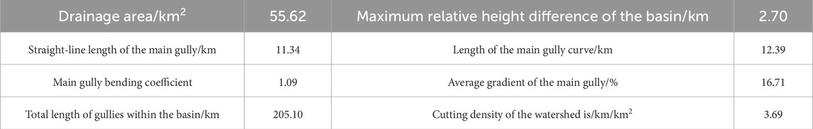
Table 1. Geometric characteristic parameters of Xulong Gully.

The Xulong Gully small watershed is located downstream of the Xulong Hydropower Station, featuring high mountains and deep valleys, belonging to a typical canyon landform type. Located on the southeastern margin of the Qinghai-Tibet Plateau and the northern Hengduan Mountains, the study area has experienced rapid uplift due to neotectonic activity since the Quaternary, with rates reaching up to 5 mm/year. Xulong Gully experiences a subtropical dry-hot valley climate characterized by distinct dry and wet seasons. The annual maximum, minimum, and average temperatures are 36 °C, −8.9 °C, and 14.6 °C, respectively, with the mean annual precipitation is 363.3 mm. Climatic variability in the region is influenced by latitude, monsoonal patterns, elevation, and topography, resulting in relatively complex conditions. Debris flows in Xulong Gully are classified as runoff-generated (Coe et al., 2008; Imaizumi et al., 2006), initiated by the mobilization of loose deposits (e.g., Quaternary paleo-sediments and gravels) through intensive rainfall-induced surface runoff and channel erosion. This mechanism differs from landslide-induced debris flows (Iverson, 1997), which transform from pre-existing landslides. Field surveys confirm the absence of large-scale landslides within the gully, supporting the runoff-generated origin.

3 Materials and methods

3.1 Mountain rainfall formula

In addition to being influenced by latitude and longitude, mountain rainfall is affected by multiple factors such as elevation difference, mountain orientation, and topography. Fu (1992) observed that at lower elevation, mountain rainfall exhibits a positive correlation with elevation, that is, the higher the elevation, the greater the rainfall. Upon reaching a certain altitude, rainfall reaches the maximum value; beyond this point, it begins to decrease. Therefore, Fu proposed the following mountain rainfall formula:

$P_Z=-a{Z}^2+2aHZ\left[P_h-a\left(2H-h\right)h\right](1)$

In the formula, Pz represents the fitted rainfall at location Z, and Ph denotes the measured rainfall at elevation h. H is the height at which maximum rainfall occurs, whereas a serves as an empirical coefficient. The conventional approach involves trial calculations using varying H values, substituting corresponding a and b coefficients (note: the original text may contain a typographical error, as b was not previously defined and likely refers to another coefficient within the formula). The optimal mountain rainfall formula for the study area is determined when the correlation coefficient reaches its maximum.

The specific calculation process of Equation 1 is as follows:

1. Data collection: Obtain the measured rainfall amounts (Ph₁, P_h2, …, P_hn) from meteorological stations (or observation points) at different altitudes (h₁, h₂, …, h_n) in the study area.

2. Setting candidate values for H: Based on the understanding of the study area (such as known empirical values of similar mountain ranges), estimate the possible range where the maximum rainfall height H may occur (for example, from 1,500 m to 2,500 m). Generate a series of candidate values for H (such as 1,500, 1,600, …, 2,500).

3. For each candidate value of H:

Establish the system of equations: Substitute each measured point (h_i, P_hi) into Equation 1. Note that P_h and h here refer to P_hi and h_i of this specific measured point. An equation is obtained for each measured point. At this time, the only unknown in the equation is a.

4. Fitting and solving for a:

Since there is only one unknown parameter a but multiple measured points (multiple equations), this usually constitutes an optimization problem. Linear regression (least squares method) is generally used to find the value of a that minimizes the sum of squared errors between the calculated values P_Z of all measured points and the measured values P_hi.

However, this fitting method entails a substantial computational burden and relatively low accuracy. Building upon this framework, (Yan, 1987) introduced a definition for the average rainfall increase rate as Equation 2:

$\delta =\frac{P_Z-P_h}{Z-h}(2)$

Herein, δ represents the average rate of change of rainfall caused by a unit height increase (or decrease) within the height interval from the reference point height h to the target point height Z.

Therefore, the rainfall formula of the Fu Baopu Mountain can be transformed into the following form Equation 3:

$\delta =-aZ+a\left(2H-h\right)(3)$

Through parameter transformation, δ is formulated without unknown variables, enabling direct computation from observed data. This approach improves the objectivity of fitted parameters and boosts computational efficiency, though it slightly reduces fitting precision. In mountain rainfall research, Jiang (1988) observed that the rainfall increment rate follows distinct patterns: slow growth at the mountain base, accelerated increase along the slopes, and a decline after surpassing the elevation of maximum rainfall. Such a curve with an inflection point and a maximum value is extremely similar to a Gaussian curve, and can be specifically described by the characteristics of three stages: in the gentle increase zone at the foot of the mountain (Z < H_inflection), the topographic lifting effect initially appears, and the precipitation increases gently; in the rapid increase zone on the mountain slope (H_inflection < Z < H), the topographic forced lifting intensifies, and the precipitation growth rate reaches its peak; in the post-peak decreasing zone (Z > H), water vapor is exhausted, and precipitation decreases with height.

Wherein, H_inflection is the inflection point height, referring to the critical elevation where the sign of curvature changes on the vertical distribution curve of mountain precipitation (P-^Z curve). It is specifically manifested as Equation 4:

${\left.\frac{d^{2}P}{d{Z}^2}\right|}_{Z=H_{\text{inflection}}}=0(4)$

That is, the rate of change of the precipitation growth rate with elevation reaches an extreme value at this point.

Such nonlinear processes can be described by a Gaussian function:

$P_Z\propto e^{-\frac{{\left(Z-\mu \right)}^2}{2{\sigma }^2}}(5)$

In the Equation 5, μ is the peak position (corresponding to H), and σ controls the width (reflecting the precipitation concentration).

Leveraging this insight, Jiang (1988) adopted a Gaussian curve for mountain rainfall fitting, expressed by the following formula:

$P_Z=a{e}^{-b{\left(Z-H\right)}^2}+c(6)$

Among them, b is the efficiency factor for terrain uplift, C controls the concentration factor of precipitation, and C is the amplitude parameter, enhancing the flexibility of the fitting. Given that the rainfall at infinity is zero, Equation 6 can be further simplified as Equation 7:

$P_Z=a{e}^{-b{\left(Z-H\right)}^2}(7)$

Equation 5 is linearized as Equation 8:

$\ln P_Z=lna-b{\left(Z-H\right)}^2(8)$

By assigning various values to H and integrating measured rainfall data, the model fits lnP_Z against (Z-H)²; through selection of the optimal fitting result, the corresponding mountain rainfall formula can be derived.

3.2 Runoff volume calculation

The runoff volume in this study is calculated using the SCS-CN method, a widely - recognized hydrological model. This method is selected for its ability to integrate hydrologic soil groups (HSG), land use types, and antecedent moisture conditions (AMC), which align with the complex geological and vegetation characteristics of Xulong Gully. Field surveys confirm that HSG in the area (e.g., low-permeability bedrock, loose deposits) and distinct land use zonation (bare soil, brush-forbs, woods) are well-represented by the method’s parameters. Designed to estimate direct surface runoff from rainfall events, the SCS-CN method accounts for soil type, land use, and AMC. It utilizes the following formula to establish the fundamental relationship between rainfall and runoff (Bartlett et al., 2017; Jiao et al., 2015; Singh et al., 2015), which is crucial for hydrological analysis, flood prediction, and water resource management. This relationship provides a practical means of quantifying the portion of precipitation that becomes runoff, an essential component in understanding the hydrological cycle of a given area.

$\mathrm{P}={\mathrm{I}}_{\mathrm{a}}+\mathrm{F}+\mathrm{Q}(9)$

$\frac{\mathrm{Q}}{\mathrm{P}-{\mathrm{I}}_{\mathrm{a}}}=\frac{\mathrm{F}}{\mathrm{S}}(10)$

${\mathrm{I}}_{\mathrm{a}}=\lambda S(11)$

In the formula, P denotes the total precipitation (mm), I_a represents the initial loss (mm), F indicates the cumulative infiltration (mm), Q implies the direct runoff (mm), S signifies the potential maximum interception (mm), and λ acts as the initial loss coefficient. By integrating Equations 9–11, the generalized expression of the SCS-CN method can be derived as Equation 12:

$\begin{array}{c}\mathrm{Q}=\frac{{\left(\mathrm{P}-{\mathrm{I}}_{\mathrm{a}}\right)}^2}{\mathrm{P}-{\mathrm{I}}_{\mathrm{a}}+\mathrm{S}}\mathrm{P}>{\mathrm{I}}_{\mathrm{a}}\\ \mathrm{Q}=0\mathrm{P}<{\mathrm{I}}_{\mathrm{a}}\end{array}(12)$

The parameter S can be expressed as Equation 13:

$\mathrm{S}=\frac{25400}{\text{CN}}-254(13)$

Among them, the unit of S is mm, and CN is a curve parameter that depends on land use, hydrological and soil types, and hydrological conditions.

3.3 Peak flood flow calculation

The isochrone method serves as the primary approach for computing clear water peak discharge. Within a watershed, net rainfall generated simultaneously across different regions does not reach the drainage section simultaneously; rainfall from certain locations requires more time to concentrate, whereas that from other areas arrives more swiftly. Isochrones are defined as lines connecting points with identical concentration times. In this study, isochrones are established according to the concentration time of Xulong Gully. First, determine the equal-flow time lines. The equal-flow time lines refer to the lines connecting the points within the basin where the net rainfall reaches the outlet section at the same time. It is necessary to first determine the flow convergence speed based on the terrain, landform, soil, vegetation and other characteristics of the basin, combined with hydrological data. Then, based on the flow convergence speed and the distance from each point to the outlet section, several equal-flow time lines should be divided. Each equal-flow time line should correspond to a consistent flow convergence time interval (i.e., equal-flow time interval), which is set as Δt. Subsequently, these isochrones are employed to calculate the clear water peak discharge for the entire watershed. The detailed procedures and methodologies are presented as follows (Sun et al., 2019; Khodnenko et al., 2018; Wang et al., 2023):

$L=\frac{l^{0.8}{\left(S+25.4\right)}^{0.7}}{7069Y^{0.5}}(14)$

$Tc=\frac{5}{3}L(15)$

In the Equations 14, 15, L represents the lag period in hours, Tc denotes the concentration time measured in hours, l stands for the concentration length in meters, Y is the average land slope percentage of the watershed, and S indicates the maximum potential retention in millimeters.

Once the concentration time has been ascertained, the net rainfall time interval Δt is set to match the spacing of the isochrone interval Δτ, as Equation 16:

$N=\frac{Tc}{\Delta t}(16)$

where N represents the number of isochrones.

$l_0=\frac{l}{N}=\frac{l_{\Delta }t}{Tc}(17)$

In the Equation 17, l₀ represents the isochrone interval. Following the determination of l₀, the entire watershed is partitioned at equal intervals of l₀ starting from the watershed outlet, with the resultant dividing lines serving as isochrones.

Secondly, collect the data of net rainfall. By calculating the runoff generation for the rainfall within the watershed, the depth of net rainfall for each period can be obtained. The watershed is assumed to be segmented into N time intervals, symbolized as f (i = 1,2, … ,N). A net rainfall event spans M time intervals, denoted as h_j (j = 1,2, … ,M). Then, calculate the outflow process generated by the net rainfall in each period. Finally, add up the outflow processes of each period. The calculation time step and the isochrone time interval are represented by Δt. The total number of time intervals during which flow occurs at the watershed outlet is calculated as T = M + N-1, and the flow rate for each time interval at the outlet is denoted as Q_k (k = 1,2, … ,T). The equation for computing the clear-water peak discharge is as Equation 18:

$Q_k=\frac{h_1}{\Delta t}{f}_k+\frac{h_2}{\Delta t}{f}_{k-1}\cdots +\frac{h_k}{\Delta t}{f}_1\cdots k>N,f_k=0;k>M,h_k=0(18)$

In Bernard et al. (2025), there is a clear correlation between the calculation process of the solid-liquid peak discharge in the solid-liquid hydrograph and the runoff peak discharge. Under the condition of a fixed bed slope, the solid discharge is controlled by the runoff discharge, so the solid-liquid peak discharge is correlated with the runoff peak discharge. This is because the flow velocity increases with the increase of the triggering liquid discharge, which in turn leads to the rise of the solid discharge, resulting in a correlation between the solid-liquid peak discharge and the runoff peak discharge. Secondly, the solid-liquid peak discharge can be calculated through the runoff peak discharge. For the formed solid-liquid surge, its hydrograph shows a peaked shape, and the peak discharge is much larger than the runoff peak discharge. The “Hydrological Calculation Manual of Sichuan Province” also indicates that the peak flow of debris flows is controlled by the peak flow of clear water. Thus, the peak discharge of debris flows during rainstorms is computed using the proportion method, which assumes that the recurrence interval of clear-water peak flow aligns with that of debris flows. This method involves augmenting the clear-water peak discharge with solid materials according to a specific ratio. By incorporating the blockage coefficient, the peak discharge of debris flows can be determined. The relevant calculation formula is as follows (Qaiser, 2021):

$Q_c=\left(1+\varphi \right)·Q_{\rho }·D_c(19)$

In the Equation 19, Q_c stands for the debris flow peak discharge, whereas Q_p denotes the clear-water peak discharge. The term 1+φ functions as the flow correction coefficient, and D_c represents the blockage coefficient.

To derive the solid–liquid hydrograph for hydraulic routing (Barbini et al., 2024), the clear-water hydrograph is initially obtained using the isochrone method. Based on field measurements of debris flow density (1.40–1.60 t/m³) and solid content (gravel, cobbles, and coarse sand), the solid–liquid ratio is determined as 1+φ = 1.565, and the blockage coefficient as D_c = 1.8 (DZ/T 0020-2006). Finally, the peak flow of the debris flow was calculated according to Equation 19.

During the simulation process, the flow process curve is set to control the flow and time in the numerical simulation. In reality, the process curve of a debris flow is complex and often has pulsation, which is related to the intermittent nature of the debris flow process. Debris flows are classified based on their source of energy as rainstorm-type debris flows and glacier meltwater-type debris flows. The latter are mostly distributed in mountain glacier areas. This study focuses on rainstorm-type debris flows. It is generally believed that the outbreak frequency of such debris flows is in correspondence with the frequency of precipitation, and the peak flow can be simplified as a triangle or a pentagon for calculation. It is considered to be a single-peak process (LIU Rui-hua et al., 1998). In this study, it is generalized as a pentagon model. By calculating several key points of a debris flow outbreak, taking one-third of the time of the debris flow as the dividing point, and using 1/4 and 1/3 of the peak flow as the debris flow flow at these two time points (Xue-jian, 2016), the flow process line of the debris flow outbreak is drawn.

3.4 Calculation of area impacted by debris flows

The impact scope of debris flows is simulated using SFLOW, a shallow water flow numerical simulation software developed by Jilin University based on the finite volume method. This study selected SFLOW for several reasons tailored to the characteristics of Xulong Gully. First, the finite volume method excels at handling complex topographies, critical in this case due to the gully’s steep gradients, deep valleys, and irregular channel geometry. It ensures numerical stability when simulating debris flow propagation across rugged terrain. Second, SFLOW uses depth-averaged equations specifically designed for shallow water flows, aligning well with the low-viscosity debris flow characteristics observed in Xulong Gully. Different from tools optimized for high-viscosity lahars or landslides, SFLOW accurately captures the fluid-like motion and deposition processes of the debris flows in this study. In addition, SFLOW allows flexible parameterization of key factors such as bed roughness and yield strength, which were calibrated using field data from Xulong Gully. This adaptability to local conditions, combined with its proven performance in simulating similar mountainous debris flow events, made it the optimal option over other available tools.

Grounded in a balanced Godunov-type finite volume algorithm, SFLOW simulates debris flow motion by solving shallow water equations. These equations include the depth-averaged mass conservation and momentum conservation equations, which can be expressed as Equation 20 (Sun et al., 2022b):

$\frac{\mathrm{\partial }q}{\mathrm{\partial }t}+\frac{\mathrm{\partial }f}{\mathrm{\partial }x}+\frac{\mathrm{\partial }g}{\mathrm{\partial }y}=s(20)$

In the formula, t denotes time, whereas x and y represent the coordinates in the x-direction and y-direction of the Cartesian coordinate system, respectively. The vectors q, f, g, and s signify the conserved variables, the x-direction numerical flux, the y-direction numerical flux, and source term, respectively. These vectors are expressed as Equation 21:

$q=\left[\begin{array}{c}h\\ q_x\\ q_y\end{array}\right]=\left[\begin{array}{c}h\\ uh\\ vh\end{array}\right]f=\left[\begin{array}{c}uh\\ u^{2}h+\frac{1}{2}g{h}^2\\ uvh\end{array}\right]g=\left[\begin{array}{c}vh\\ uvh\\ v^{2}h+\frac{1}{2}g{h}^2\end{array}\right]\mathit{s}=\left[\begin{array}{c}0\\ -gh\frac{\mathrm{\partial }{z}_b}{\mathrm{\partial }x}-S_{fx}\\ -gh\frac{\mathrm{\partial }{z}_b}{\mathrm{\partial }y}-S_{fy}\end{array}\right](21)$

Currently, many researchers have proposed their own friction models for handling the bed friction term in shallow water flow, such as the Coulomb friction model, Voellmy friction model, and Quadratic Rheological friction model (George and Iverson, 2014; Rickenmann et al., 2006). Among them, the Quadratic Rheological friction model takes into account the internal viscosity and turbulence effects of shallow water flow fluid, and it is currently widely used to handle the bed friction term in the shallow water flow equations. Its expression is as Equation 22 (Chen et al., 2017):

$S_f=S_1+S_2+S_3=\frac{\tau }{{\rho }_m}+\frac{K\beta U}{8{\rho }_{m}h}+\frac{g{n}_{td}^2{U}^2}{h^{1/3}}(22)$

Wherein: S_f represents the bed friction term; S₁ represents the fluid yield factor; S₂ represents the fluid viscosity factor; S₃ represents the fluid turbulent diffusion factor; τ represents the fluid yield strength; ρ_m represents the solid density of the solid-phase deposits formed after the shallow water flow rushes out; K represents the shallow water flow layer resistance coefficient; represents the shallow water flow fluid viscosity; U represents the shallow water flow velocity; n_td represents the equivalent Manning resistance coefficient. The difference between this coefficient and the traditional Manning coefficient is that it takes into account the inherent collision factors within the fluid. The empirical relationship between it and the traditional Manning coefficient is as Equation 23:

$n_{td}=0.0538n_m\mathit{exp}\left(6.0896C_V\right)(23)$

Wherein: n_m represents the traditional Manning coefficient; C_V represents the solid-phase volume concentration of the shallow water flow fluid.

In addition, based on Equation 22, the bed friction terms in the x and y directions, S_fx and S_fy, can be derived:

$S_{fx}=\frac{\tau }{{\rho }_m}+\frac{K\beta u}{8{\rho }_{m}h}+\frac{g{n}_{td}^2{u}^2}{h^{1/3}}(24)$

$S_{fy}=\frac{\tau }{{\rho }_m}+\frac{K\beta v}{8{\rho }_{m}h}+\frac{g{n}_{td}^2{v}^2}{h^{1/3}}(25)$

In the Equations 24, 25, h represents the depth of shallow water flow, Z_b indicates the elevation of the bottom bed within the simulated domain, and g denotes the acceleration due to gravity. q_x and q_y are the single-width flow rates in the x- and y-directions, respectively, and are the bed slopes in the x and y directions, respectively. S_fx and S_fy are the friction coefficients of the bottom bed in the x and y directions, respectively. The debris flow peak discharge (Qc) is input into SFLOW as part of a hydrograph, which describes the temporal variation of flow rate (with Qc as the peak value). This hydrograph is assigned to the inflow boundary of the simulation domain (the gully head in Xulong Gully). Combined with topographic data (DEM) and parameters like bed friction and yield strength, SFLOW solves the shallow water equations to simulate debris flow routing, including the evolution of flow depth, velocity, and area impacted by debris flow.

In the SFLOW software, the boundary conditions and calculation domain for numerical simulation are determined according to the actual conditions of the study area. The governing equations are solved using a digital elevation model (DEM). In addition, the software requires setting the inflow and outlet of the debris flow as inflow points when defining boundary conditions.

4 Results

4.1 Fitting result of the mountain rainfall formula

Due to the influence of the foehn effect, precipitation in Xulong Gully demonstrates distinct vertical distribution characteristics. Despite the numerous meteorological stations in Yunnan and Sichuan provinces, the majority are concentrated in towns rather than along the Jinsha River. Statistical data indicate that three meteorological stations exist within a 100-km radius of Xulong Gully, six stations within 200 km, and 24 stations within 300 km. Considering factors such as station location, climate zones, slope aspect, and proximity to Xulong Gully, rainfall data from 10 meteorological stations with climatic conditions analogous to those of Xulong Gully were selected to fit the mountain rainfall formula, as presented in Table 2.

Table 2

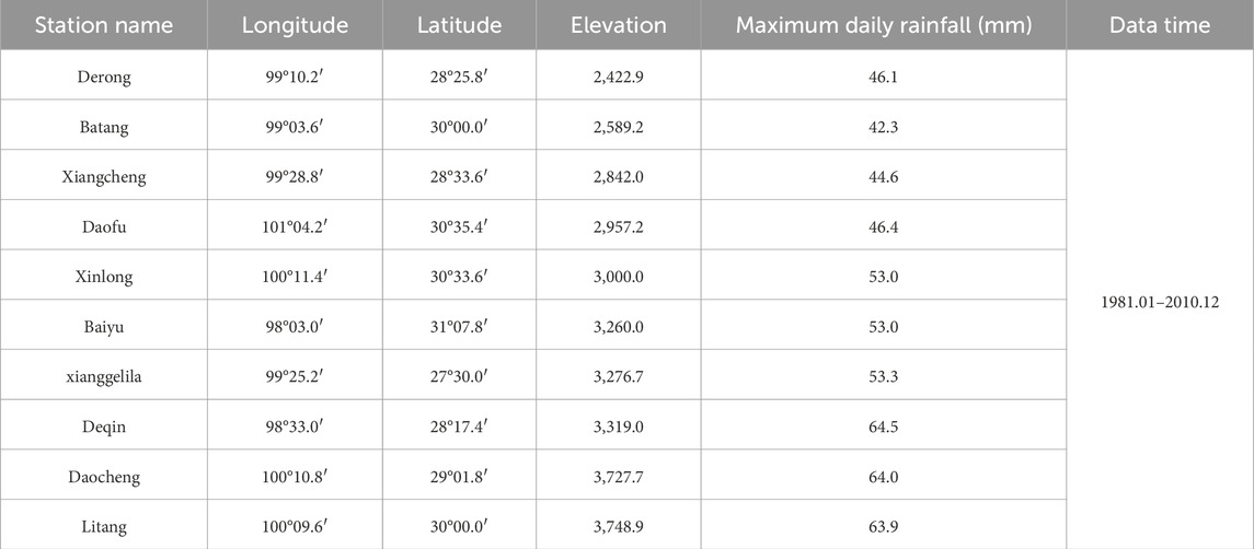
Table 2. Statistical table of maximum daily rainfall of weather stations at different altitudes.

The vertical distribution characteristics of precipitation in Xulong Gully were fitted using the daily maximum rainfall data from the aforementioned meteorological stations and integrating the mountain rainfall formula. The calculation parameters and results are detailed in Table 3 (Sun et al., 2018), whereas the computed vertical rainfall distribution characteristics of Xulong Gully are illustrated in Figure 2.

Table 3

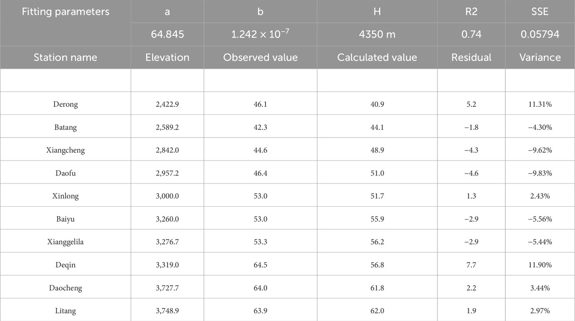
Table 3. Fitting results of mountain rainfall formula.

Figure 2

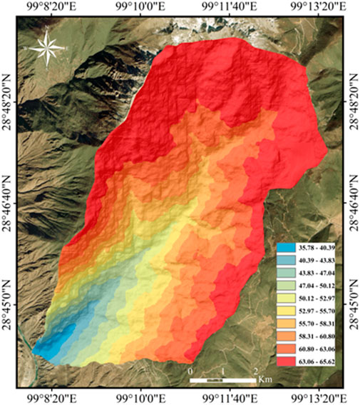
Figure 2. Fitting result of the mountain rainfall formula.

As shown in Table 3, the fitting results yield a linear correlation coefficient of 0.74, a sum of squared errors of 0.05794, and a maximum precipitation elevation H of 4,350 m, consistent with field measurements. The relative error in fitting Deqin’s maximum daily rainfall is 11.90%, whereas the minimum relative error for Xinlong’s maximum daily rainfall is 2.43%. The fitting outcomes aligns well with the rainfall distribution characteristics of Xulong Gully as determined through field investigations.

4.2 Calculation result of runoff volume

4.2.1 Hydrologic soil groups (HSG)

Through field surveys and data compilation, the hydrologic soil groups within the Xulong Gully watershed were characterized. Bedrock outcrops are present near the gully outlet: quartz diorite defines the right-bank lithology, whereas gneiss underlies the left-bank bedrock, both exhibiting low permeability. Between elevations of 2,100 and 3,300 m, Quaternary-era paleo-sediments are observed, comprising unconsolidated gravel or cobble frameworks with clay/sand infill, and exhibiting relative stability. Brown soil, with an average permeability of 2.43 × 10⁻⁶ cm/s, predominates in the 3,300–4,200 m zone. Marble bedrock emerges between 4,200 and 4,500 m, transitioning to plateau snowfields above 4,500 m. Loose deposits and cultivated lands are sporadically distributed throughout localized areas. The spatial distribution of hydrologic soil groups in the study area is visualized in Figure 3 (Sun et al., 2019).

Figure 3

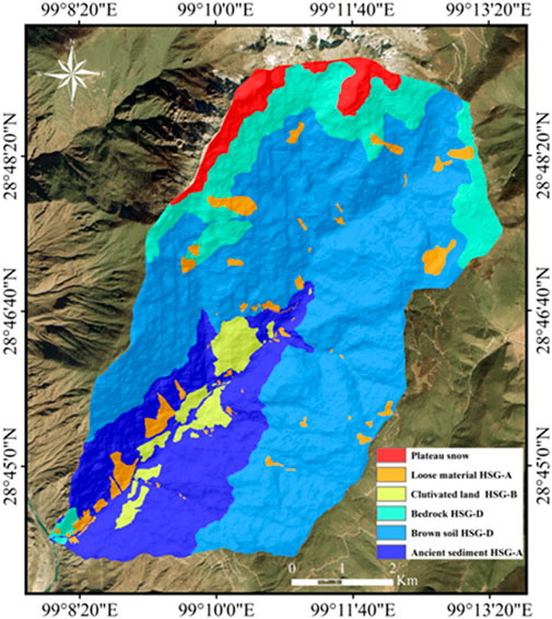
Figure 3. Distribution characteristics of HSG in Xulong Gully (Sun et al., 2019).

4.2.2 Land use type

Field investigations reveal distinct vegetation zonation in Xulong Gully based on elevation. Bare soil dominates the 2,100–2,500 m zone; brush-forbs cover elevations from 2,500 m to 3,300 m; woods are prevalent between 3,300 and 4,200 m range; grasslands occur between 4,200 and 4,500 m; plateau snowfields prevail above 4,500 m. Moreover, scattered patches of loose deposits and cultivated land are interspersed throughout the watershed (Sun et al., 2019). The spatial distribution of these vegetation types is presented in Figure 4.

Figure 4

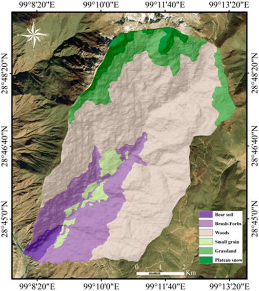
Figure 4. Distribution characteristics of land use in Xulong Gully (Sun et al., 2019).

4.2.3 Runoff volume

The SCS-CN method demonstrates pronounced sensitivity to the curve number (CN), underscoring the critical importance of its accurate determination. The CN value is fundamentally governed by three interrelated factors: HSG, land use characteristics, and AMC. Specifically, AMC serves as a key indicator of antecedent soil moisture status and is typically quantified using cumulative precipitation over the preceding 5-day period (Sun et al., 2018).

Based on the cumulative 5-day antecedent rainfall, AMC conditions are systematically categorized into three distinct classes:

a. AMC I: Total rainfall less than 35 mm, indicating relatively dry soil conditions.

b. AMC II: Rainfall between 35 and 53 mm, representing intermediate moisture conditions.

c. AMC III: Rainfall exceeding 53 mm, denoting wet soil conditions.

Notably, due to reliance on rainfall data from a single meteorological station, the analysis was restricted to evaluating curve numbers under AMC-II conditions. For each grid cell within the study area, the CN value was determined by integrating HSG classifications, land use types, and precipitation inputs, as visualized in Figure 5. Subsequently, Equation 11 was used to compute runoff depth (expressed in mm/day), with the results illustrated in Figure 6. This approach ensures systematic integration of hydrological parameters to characterize the rainfall–runoff relationship with enhanced precision.

Figure 5

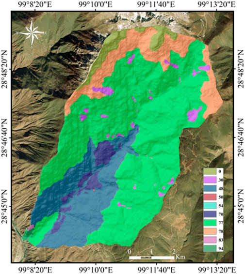
Figure 5. Distribution characteristics of CN value in Xulong Gully (Sun et al., 2019).

Figure 6

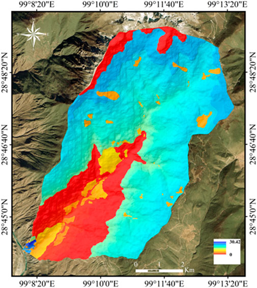
Figure 6. Distribution characteristics of runoff in Xulong Gully (Sun et al., 2019).

4.3 Calculation results of peak flow of debris flow

Utilizing the digital elevation model (DEM) of Xulong Gully alongside field survey data, the isochrone method was employed to compute the clear-water peak discharge, incorporating runoff estimates derived using the SCS-CN model. The DEM, with a spatial resolution of 5 × 5 m, was used to extract fundamental parameters, including the average channel slope and length of Xulong Gully (Table 4). Equations 12, 13 were applied to calculate the watershed concentration time, followed by determining the area distribution within each isochrone interval. Finally, Equation 16 was used to derive the flood hydrograph, deriving the clear-water peak discharge (Table 5).

Table 4

Table 4. Basic parameters of calculation using the isocurrent time-line method.

In debris flow evaluations, traditional approaches often rely on rainfall data from a single meteorological station near or within the study area to estimate flood or debris flow peak discharges (as specified in the Geological Survey Specifications for Debris Flow Stability, DZ/T 0020-2006). In addition, some scholars have explored the impact of non-uniform rainfall distribution on peak discharge calculations, using interpolation methods to simulate spatial variability in precipitation. To enhance the accuracy of peak flow prediction model for Xulong Gully, this study applied the traditional method using data exclusively from the Derong meteorological station, and an interpolation method using IDW. These rainfall inputs were integrated with the isochrone method to calculate the clear-water peak discharge of Xulong Gully (Table 5).

Table 5

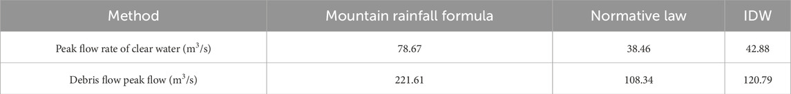
Table 5. Peak discharge of clear water and debris flow in Xulong Gully.

Field investigations reveal that the Xulong Gully channel is relatively straight, with minimal steep banks or constrictions, a scattered formation area, and general riverbed blockage. The debris flow exhibits a thick slurry state (1.40–1.60 t/m³). Based on these conditions and in accordance with the Specifications for Geological Survey of Debris Flow Stability (DZ/T 0020-2006), the blockage coefficient is determined to be 1.8, and the debris flow discharge correction coefficient is 1.565. The peak debris flow discharge for Xulong Gully can be obtained using Equation 17 (Table 5).

4.4 Calculation results of the area impacted by debris flows

The non-slurry component of the debris flow fluid consists primarily of stones, gravel, and coarse sand, with minimal fine-grained material—especially extremely low silty-clay content—indicating that the debris flow exhibits low-viscosity behavior. Therefore, a viscosity coefficient of 10 Pa·s is adopted for numerical simulation. The solid density of the debris flow, referring to the medium density of soil with stones, is regarded as 2,650 kg/m³. The Xulong Gully riverbed is composed of pebbles and boulders, including large boulders, with a generally uniform bottom but an uneven bed surface. Therefore, the channel roughness coefficient in the flow zone is set to 0.04. Field investigations indicate that the thickness of historical debris flow fan residues at the outlet of Xulong Gully is 10 m ±, justifying the use of a higher yield strength of 10 kPa in the viscosity-related calculations. In addition, the interlayer friction coefficient of the debris flow fluid is assigned an empirical value of 2,500. The starting point of the debris flow is selected as the beginning of the flow zone.

Xulong Gully is located within a subtropical dry–hot valley climate zone, where debris flows are predominantly triggered by intense rainstorms. These flows are consistent with flood processes, confirming their classification as runoff-generated debris flows (Coe et al., 2008), in which water and solid particles are entrained synchronously by concentrated surface runoff. The flood hydrograph is simplified as a single-peak process, typically represented by a pentagonal or triangular form (Bao et al., 2019). In this study, the debris flow hydrograph is modeled using a pentagonal shape. Taking one-third of a debris flow process as the demarcation point, and assigning one-fourth and one-third of the peak discharge as the flow rates at the two demarcation points, the resulting debris flow hydrograph, shown in Figure 7, integrates liquid (water) and solid (particles) components, following the method of (Barbini et al., 2024). The rising and falling limbs of the hydrograph reflect the dynamic entrainment and deposition of solids, consistent with the runoff-generated debris flow mechanism.

Figure 7

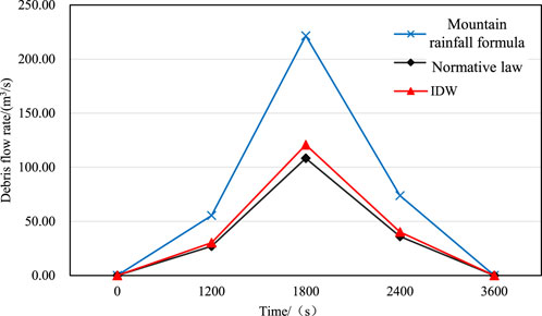
Figure 7. Process curves of debris flow under different rainfall distribution conditions.

The area impacted by debris flows, flow depth, and flow velocity of debris flows under different rainfall distribution conditions in Xulong Gully were calculated using the SFLOW software. The results were processed using ArcGIS software to visually observe the hazard extent of debris flows in Xulong Gully (Figure 8).

Figure 8

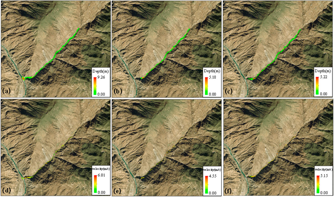
Figure 8. Outflow range, flow depth and flow velocity of debris flow in Xulong Gully under different rainfall distribution conditions: (a) outflow range and flow depth calculated using the mountain rainfall formula; (b) extent and depth calculated using the standard method; (c) range and depth calculated using the IDW method; (d) flow velocity calculated using the mountain rainfall formula; (e) flow velocity calculated using the normative method; (f) flow velocity calculated using the IDW method.

5 Discussion

5.1 Comparative analysis of peak flow of debris flow

Table 5 illustrates that the debris flow peak discharge of Xulong Gully calculated using the mountain rainfall formula is 221.61 m³/s, whereas the code-based method yields 108.34 m³/s, and the IDW method results in 120.79 m³/s. Compared with the mountain rainfall formula method, the average errors of the code-based and IDW methods are 47.53% and 54.51%, respectively. Thus, the peak discharge calculated by the mountain rainfall formula is approximately twice that of the code-based and IDW methods. This finding indicates that the vertical distribution characteristics of rainfall in Xulong Gully have a significant impact on the calculation of debris flow peak discharge. If only the rainfall data from the meteorological station closest to Xulong Gully, as specified in the code-based method, is used, the hazard of debris flows will be greatly underestimated. Although the peak discharge calculated by the IDW method exhibits remarkable improvement compared with the code-based method, it often fails to capture the influence of micro-topography on rainfall distribution in watersheds such as Xulong Gully, and can only reflect the rainfall distribution characteristics of larger areas.

The differences in debris flow peak discharges between methods stem from how rainfall distribution is characterized. The mountain rainfall formula accounts for vertical variability by fitting precipitation to a Gaussian curve that peaks at 4,350 m (Table 3), capturing higher rainfall in upper elevations where loose deposits, (a key material source, are abundant. This condition results in greater runoff and a higher clear-water peak (78.67 m³/s), which, when adjusted using correction/blockage coefficients, yields a debris flow peak of 221.61 m³/s.

By contrast, the traditional method relies solely on data from Derong Station (2,422.9 m), underestimating rainfall in upper zones. The IDW method interpolates sparse station data but overlooks topographic controls such as the foehn effect, failing to capture elevation-driven increases in rainfall. Both approaches result in lower clear-water peaks (38.46 and 42.88 m³/s), and consequently, smaller debris flow discharges. These discrepancies highlight that neglecting vertical rainfall distribution underestimates high-elevation rainfall contribution to runoff and debris flow volume in this topographically complex gully.

5.2 Analysis of numerical simulation results

As shown in Figure 8, the numerical simulation results of the area impacted by debris flows, flow depth, and flow velocity in Xulong Gully under different rainfall distribution characteristics are presented. The movement paths of debris flows calculated by the code-based and IDW methods generally follow the flow zone of the Xulong Gully watershed. The thickness of debris flow deposits varies slightly, with maximum deposition thicknesses of 5.18 and 5.22 m, respectively, and approximately 1.5 m in the gully. However, results calculated using the mountain rainfall formula method show that debris flow deposits in Xulong Gully extend to the Jinsha River basin at the gully outlet, forming an distinct deposition fan. The deposit thickness increases significantly, with a maximum of 9.26 m and an average of 2.5 m ± in the main gully. The deposition fan extends nearly 300 m beyond the gully outlet. Near the outlet, steep drop topography intensifies deposition, sharply increasing deposit thickness. The area impacted by debris flows calculated using the mountain rainfall formula extends beyond the outlet of Xulong Gully, forming a large-scale deposition fan that may obstruct the Jinsha River channel and cause temporary river closure. This condition poses significant threats to the Xulong Hydropower Station located 2 km upstream, as well as to downstream villages, towns, and highways. However, the area impacted by debris flows calculated using the code-based and IDW methods do not reach the gully outlet, substantially underestimating the hazard degree of debris flows in Xulong Gully.

In the flow velocity distribution map (Figure 8), the maximum debris flow velocities in Xulong Gully calculated using the code-based and IDW methods are 4.66 and 5.15 m/s, respectively, whereas the mountain rainfall formula yields a higher maximum velocity of 6.01 m/s. This finding suggests that debris flows modeled using the mountain rainfall formula method possess greater flow energy within the main gully, resulting in higher impact force and destructive potential. Similarly, the flow velocities derived from the code-based and IDW methods underestimate the dynamic intensity and destructive capacity of debris flows in Xulong Gully.

Notably, the current SFLOW simulation does not consider flow avulsion, which may affect predictions of impacted area in complex terrains (De Haas et al., 2018; Schiavo et al., 2024). Field observations reveal localized bank instability in the downstream channel of Xulong Gully (e.g., loose deposit slopes with gradients >30°), which may initiate avulsion during high-magnitude debris flow events. Future studies will integrate channel bed erosion/deposition models and lateral instability criteria (Schiavo et al., 2024) to simulate potential avulsion processes, improving the accuracy of hazard zoning.

It is worth noting that a notable limitation of this study is the lack of direct validation against observed debris flow events. Our simulations focus on predicting potential debris flow impacts under vertical rainfall distribution, rather than reconstructing specific historical events. Consequently, on-site observational data (e.g., actual runout area, deposition thickness, or peak discharge during real debris flow events) are unavailable for model calibration and validation. However, if a debris flow event occurs in Xulong Gully, immediate field investigations can be conducted to collect key data (Frank et al., 2015; Gregoretti et al., 2019). Such data include the actual area impacted by debris flow, deposition characteristics (e.g., thickness, material composition), and flow dynamics (e.g., velocity, peak discharge). These first-hand observations will enable us to refine the hydraulic model parameters (e.g., friction coefficients, yield strength). They will also improve the accuracy of our prediction framework, thereby enhancing the reliability of the study’s conclusions.

5.3 Debris flow hazard mapping

The hazard zoning of debris flows can be carried out using the debris flow depth. In this study, the hazard degree of debris flows in Xulong Gully is classified as follows: 0.0–1.0 m as low hazard, 1.0–2.0 m as moderate hazard, 2.0–3.0 m as high hazard, and above 3.0 m as extremely high hazard. The zoning results are shown in Figure 9.

Figure 9

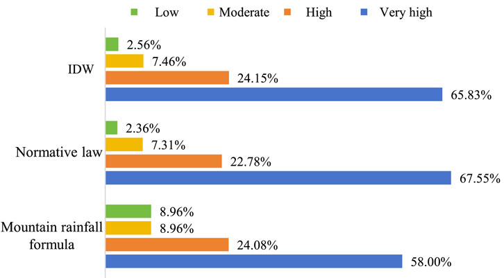
Figure 9. Statistics table of debris flow risk mapping.

The zoning results suggest that all three methods predominantly classify the area as low- and moderate-hazard zones. The low-hazard areas calculated by the mountain rainfall formula, code-based method, and IDW method account for 58.00%, 67.55%, and 65.83%, respectively, whereas the moderate-hazard areas account for 24.08%, 22.78%, and 24.15%, respectively. However, the proportions of high and extremely high hazard zones calculated by the mountain rainfall formula method are significantly greater than those derived from the code-based and IDW methods, both accounting for 8.96%. These high and extremely high hazard areas are primarily concentrated near the outlet of the Xulong Gully watershed. To facilitate a more intuitively comparison of debris flow hazard levels in Xulong Gully under different rainfall distribution conditions, a Hazard Index (HI) is introduced. The calculation formula for HI is as Equation 26:

$HI=\frac{Higharea+Veryhigharea}{TotalArea}(26)$

The calculated HI values for the mountain rainfall formula method, code-based method, and IDW method are 17.92, 9.67, and 10.02, respectively. These results reveal an increasing trend in HI values from the code-based method to the IDW method, and then to the mountain rainfall formula method. Notably, the HI value derived from the mountain rainfall formula method is significantly higher than those obtained from the IDW and code-based methods. This finding indicates that the mountain rainfall formula method estimates a greater debris flow hazard in Xulong Gully, whereas the IDW and code-based methods underestimate the hazard severity.

6 Conclusion

This study employs the Gaussian rainfall formula to characterize the vertical distribution of rainfall in Xulong Gully. The peak discharge of debris flows under varying rainfall distribution scenarios is calculated using the isochrone method. Subsequently, the impacted area, flow depth, and flow velocity of debris flows are determined based on shallow water flow dynamics, using the finite volume method. The following conclusions are drawn:

1. The use of the code-based method and conventional interpolation techniques to estimate debris flow peak discharge presents significant limitations in regions including Xulong Gully, where rainfall is affected by micro-topography and micro-climate, exhibiting vertical distribution characteristics. The peak discharge calculated using the mountain rainfall formula method is approximately twice that obtained from the code-based and conventional interpolation methods, with average errors of 47.53% and 54.51%, respectively. These methods yield notably lower discharge estimates. Furthermore, due to the sparse distribution of meteorological stations in the study area, considerable uncertainty remains in estimating the vertical rainfall distribution. If sufficient maximum daily rainfall data can be obtained from a more comprehensive network of meteorological stations, then the Pearson-III distribution can be used to construct frequency distribution curves of maximum daily rainfall for each station. This approach would enable a more accurate determination of rainfall distribution characteristics Xulong Gully under different design frequencies.

2. The debris flow in Xulong Gully, as calculated using the mountain rainfall formula method, is capable of breaching the gully outlet and forming a deposition fan approximately 300 m in length. By contrast, debris flows estimated using the code-based and IDW methods remain confined within the main gully and do not reach the outlet, with considerably lower maximum deposition thickness. The impacted area calculated using the mountain rainfall formula method extends beyond the outlet, forming a large-scale deposition fan that poses potential hazards. This fan may obstruct the Jinsha River channel, cause temporary river closure, and affect the Xulong Hydropower Station upstream and villages/towns located downstream.

3. Based on debris flow deposition thickness, the hazard zoning results for the Xulong Gully watershed indicate that the overall debris flow hazard is generally low. The HI values calculated using the mountain rainfall formula, code-based method, and IDW method are 17.92, 9.67, and 10.02, respectively. The HI value associated with the mountain rainfall formula method suggests a more substantial debris flow hazard, whereas the IDW and code-based methods yield comparatively lower hazard assessments.

Data availability statement

The raw data supporting the conclusions of this article will be made available by the authors, without undue reservation.

Author contributions

WP: Methodology, Writing – original draft. XS: Validation, Writing – review and editing. LT: Conceptualization, Writing – review and editing.

Funding

The author(s) declare that financial support was received for the research and/or publication of this article. This research was funded by the Doctoral Research Start-up Project of Hunan University of Arts and Science (Grant No. 22BSQD20).

Acknowledgments

The authors gratefully acknowledge the editor and reviewers for their insightful comments and constructive suggestions, which greatly contributed to improving the quality and clarity of this paper.

Conflict of interest

The authors declare that the research was conducted in the absence of any commercial or financial relationships that could be construed as a potential conflict of interest.

Generative AI statement

The author(s) declare that no Generative AI was used in the creation of this manuscript.

Any alternative text (alt text) provided alongside figures in this article has been generated by Frontiers with the support of artificial intelligence and reasonable efforts have been made to ensure accuracy, including review by the authors wherever possible. If you identify any issues, please contact us.

Publisher’s note

All claims expressed in this article are solely those of the authors and do not necessarily represent those of their affiliated organizations, or those of the publisher, the editors and the reviewers. Any product that may be evaluated in this article, or claim that may be made by its manufacturer, is not guaranteed or endorsed by the publisher.

References

Bao, Y., Chen, J., Sun, X., Han, X., Li, Y., Zhang, Y., et al. (2019). Debris flow prediction and prevention in reservoir area based on finite volume type shallow-water model: a case study of pumped-storage hydroelectric power station site in Yi County, Hebei, China. Environ. Earth Sci. 78, 577. doi:10.1007/s12665-019-8586-4

CrossRef Full Text | Google Scholar

Barbini, M., Bernard, M., Boreggio, M., Schiavo, M., D'Agostino, V., and Gregoretti, C. (2024). An alternative approach for the sediment control of in-channel stony debris flows with an application to the case study of Ru Secco Creek (Venetian Dolomites, Northeast Italy). Front. Earth Sci. 12, 1340561. doi:10.3389/feart.2024.1340561

CrossRef Full Text | Google Scholar

Bartlett, M. S., Parolari, A. J., McDonnell, J. J., and Porporato, A. (2017). Reply to comment by Fred L. Ogden et al. on “Beyond the SCS-CN method: a theoretical framework for spatially lumped rainfall-runoff response”. Water Resour. Res. 53, 6351–6354. doi:10.1002/2017WR020456

CrossRef Full Text | Google Scholar

Bernard, M., and Gregoretti, C. (2021). The use of Rain Gauge measurements and radar data for the model-based prediction of runoff-generated debris-flow occurrence in Early Warning systems. Water Resour. Res. 57. doi:10.1029/2020wr027893

CrossRef Full Text | Google Scholar

Bernard, M., Barbini, M., Berti, M., Boreggio, M., Simoni, A., and Gregoretti, C. (2025). Rainfall-runoff modeling in Rocky Headwater Catchments for the prediction of debris flow occurrence. Water Resour. Res. 61. doi:10.1029/2023wr036887

CrossRef Full Text | Google Scholar

Chen, M. S. W., and Wang, Q. (2024). Research on Adaptation of local combined rainfall spatial interpolation method. Water Resour. Hydropower Eng., 1–12.

Google Scholar

Chen, H. X., Zhang, L. M., Gao, L., Yuan, Q., Lu, T., Xiang, B., et al. (2017). Simulation of interactions among multiple debris flows. Landslides 14, 595–615. doi:10.1007/s10346-016-0710-x

CrossRef Full Text | Google Scholar

Coe, J. A., Kinner, D. A., and Godt, J. W. (2008). Initiation conditions for debris flows generated by runoff at Chalk Cliffs, central Colorado. Geomorphology 96, 270–297. doi:10.1016/j.geomorph.2007.03.017

CrossRef Full Text | Google Scholar

De Haas, T., Densmore, A. L., Stoffel, M., Suwa, H., Imaizumi, F., Ballesteros-Canovas, J. A., et al. (2018). Avulsions and the spatio-temporal evolution of debris-flow fans. Earth-Science Rev. 177, 53–75. doi:10.1016/j.earscirev.2017.11.007

CrossRef Full Text | Google Scholar

Eu, S., and Im, S. (2025). The effect of entrainment model on debris-flow simulation-comparison of two Simple 1D models. Water 17, 761. doi:10.3390/w17050761

CrossRef Full Text | Google Scholar

Frank, F., McArdell, B. W., Huggel, C., and Vieli, A. (2015). The importance of entrainment and bulking on debris flow runout modeling: examples from the Swiss Alps. Nat. Hazards Earth Syst. Sci. 15, 2569–2583. doi:10.5194/nhess-15-2569-2015

CrossRef Full Text | Google Scholar

Fu, B. (1992). The effects of topography and elevation on precipitation. Acta Geogr. Sin. 000 (004), 302–314. doi:10.11821/xb199204002

CrossRef Full Text | Google Scholar

George, D. L., and Iverson, R. M. (2014). A depth-averaged debris-flow model that includes the effects of evolving dilatancy. II. Numerical predictions and experimental tests. Proc. R. Soc. a-Mathematical Phys. Eng. Sci. 470, 20130820. doi:10.1098/rspa.2013.0820

CrossRef Full Text | Google Scholar

Gregoretti, C., Stancanelli, L. M., Bernard, M., Boreggio, M., Degetto, M., and Lanzoni, S. (2019). Relevance of erosion processes when modelling in-channel gravel debris flows for efficient hazard assessment. J. Hydrology 568, 575–591. doi:10.1016/j.jhydrol.2018.10.001

CrossRef Full Text | Google Scholar

Imaizumi, F., Sidle, R. C., Tsuchiya, S., and Ohsaka, O. (2006). Hydrogeomorphic processes in a steep debris flow initiation zone. Geophys. Res. Lett. 33. doi:10.1029/2006gl026250

CrossRef Full Text | Google Scholar

Iverson, R. M. (1997). The physics of debris flows. Rev. Geophys. 35, 245–296. doi:10.1029/97rg00426

CrossRef Full Text | Google Scholar

Jiang, Z. (1988). A discussion on the mathematical model of mountain precipitation with vertical distribution. Geogr. Res. 7 (1), 349–354. doi:10.11821/yj1988010010

CrossRef Full Text | Google Scholar

Jiao, P., Xu, D., Wang, S., Yu, Y., and Han, S. (2015). Improved SCS-CN method based on storage and Depletion of antecedent daily precipitation. Water Resour. Manag. 29, 4753–4765. doi:10.1007/s11269-015-1088-6

CrossRef Full Text | Google Scholar

Khodnenko, I., Kudinov, S., and Smirnov, E. (2018). “Walking distance estimation using multi-agent simulation of pedestrian flows,” in Proceedings of the 7th annual international Young Scientists Conference on computational science (YSC), Heraklion, Greece, 489–498.

CrossRef Full Text | Google Scholar

Liu Rui-hua, Z.G.-w., Yan-ji, FENG, and Jun-hong, CHEN (1998). 97·5.8 Feilai Temple debris flow mechanism in Qingyuan, Guangdong. Trop. Geogr. (03), 232–236. doi:10.3969/j.issn.1001-5221.1998.03.009

CrossRef Full Text | Google Scholar

Liu, X., Zhang, W., Li, G., and Liu, B. (2023). Research on evolution process and impact range prediction of high level Remote Collapse and landslide-debris flow disaster Chain——taking the 4·5 Tiejiangwan geological disaster chain in hongya County,Sichuan province as an example. J. Jilin Univ. Earth Sci. Ed. 53 (6), 1799–1811. doi:10.13278/j.cnki.jjuese.20230258

CrossRef Full Text | Google Scholar

Ma, Y., and Li, C. (2017). “Research on the debris flow hazards after the Wenchuan Earthquake in Bayi gully, Longchi, Dujiangyan, Sichuan province, China,” in Proceedings of the International Conference on Advanced materials science and Civil Engineering (AMSCE), Phuket, Thailand, 166–170.

Google Scholar

Nagano, H., Hashimoto, H., and Miyoshi, T. (2013). “One-dimensional model of landslide-induced debris flow with Woody debris,” in Proceedings of the 35th world congress of the international-association-for-hydro-environment-engineering-and-research (iahr), int assoc hydro environm engn & Res, Chengdu (Chengdu, Sichuan; Tsinghua University Press).

Google Scholar

Qaiser, M. (2021). Debris flow Susceptibility assessment and runout prediction o fDatong and Taicun gullies near the first Bend of the Yangtze river. Jilin University.

Google Scholar

Rickenmann, D., Laigle, D., McArdell, B. W., and Hubl, J. (2006). Comparison of 2D debris-flow simulation models with field events. Comput. Geosci. 10, 241–264. doi:10.1007/s10596-005-9021-3

CrossRef Full Text | Google Scholar

Riley, K. L., Bendick, R., Hyde, K. D., and Gabet, E. J. (2013). Frequency-magnitude distribution of debris flows compiled from global data, and comparison with post-fire debris flows in the western US. Geomorphology 191, 118–128. doi:10.1016/j.geomorph.2013.03.008

CrossRef Full Text | Google Scholar

Schiavo, M., Gregoretti, C., Boreggio, M., Barbini, M., and Bernard, M. (2024). Probabilistic Identification of debris-flow Pathways in mountain fans within a Stochastic framework. J. Geophys. Research-Earth Surf. 129, e2024JF007946. doi:10.1029/2024jf007946

CrossRef Full Text | Google Scholar

Singh, P. K., Mishra, S. K., Berndtsson, R., Jain, M. K., and Pandey, R. P. (2015). Development of a Modified SMA based MSCS-CN model for runoff estimation. Water Resour. Manag. 29, 4111–4127. doi:10.1007/s11269-015-1048-1

CrossRef Full Text | Google Scholar

Sun, X., Liu, G., Zhao, T., Tang, L., Han, X., and Peng, W. (2025). Application of a geomorphic restoration method for landslide susceptibility mapping along the rapidly uplifting section of the upper Jinsha river, South-Western China. Bull. Eng. Geol. Environ. 84, 181. doi:10.1007/s10064-025-04213-2

CrossRef Full Text | Google Scholar

Sun, X., Chen, J., Bao, Y., Han, X., Zhan, J., and Peng, W. (2018). Landslide susceptibility mapping using Logistic regression analysis along the Jinsha River and its tributaries close to Derong and Deqin County, southwestern China. Isprs Int. J. Geo-Information 7, 438. doi:10.3390/ijgi7110438

CrossRef Full Text | Google Scholar

Sun, X., Chen, J., Bao, Y., Han, X., Zhan, J., and Peng, W. (2019). Flash flood schlep ability estimation in vertical distribution law of the precipitation area: a case of Xulong gully, Southwest China. Arabian J. Geosciences 12, 279. doi:10.1007/s12517-019-4463-4

CrossRef Full Text | Google Scholar

Sun, X., Chen, J., Han, X., Bao, Y., Zhan, J., and Peng, W. (2020a). Application of a GIS-based slope unit method for landslide susceptibility mapping along the rapidly uplifting section of the upper Jinsha River, South-Western China. Bull. Eng. Geol. Environ. 79, 533–549. doi:10.1007/s10064-019-01572-5

CrossRef Full Text | Google Scholar

Sun, X., Chen, J., Han, X., Bao, Y., Zhou, X., and Peng, W. (2020b). Landslide susceptibility mapping along the upper Jinsha River, south-western China: a comparison of hydrological and curvature watershed methods for slope unit classification. Bull. Eng. Geol. Environ. 79, 4657–4670. doi:10.1007/s10064-020-01849-0

CrossRef Full Text | Google Scholar

Sun, X., Chen, J., Li, Y., and Rene, N. N. (2022a). Landslide susceptibility mapping along a rapidly uplifting river valley of the upper Jinsha River, southeastern Tibetan plateau, China. Remote Sens. 14, 1730. doi:10.3390/rs14071730

CrossRef Full Text | Google Scholar

Sun, X., Han, X., Chen, J., Bao, Y., and Peng, W. (2022b). Numerical simulation of the Qulong Paleolandslide Dam event in the late pleistocene using the finite volume type shallow water model. Nat. Hazards 111, 439–464. doi:10.1007/s11069-021-05060-6

CrossRef Full Text | Google Scholar

Wang, F., Chen, X.-q., and Chen, J.-g. (2017). Experimental study on the energy dissipation characteristics of debris flow deceleration baffles. J. Mt. Sci. 14, 1951–1960. doi:10.1007/s11629-016-3868-8

CrossRef Full Text | Google Scholar

Wang, D., Chen, Z., He, S., Liu, Y., and Tang, H. (2018). Measuring and estimating the impact pressure of debris flows on bridge piers based on large-scale laboratory experiments. Landslides 15, 1331–1345. doi:10.1007/s10346-018-0944-x

CrossRef Full Text | Google Scholar

Wang, C., Zhao, S.-j., Ren, Z.-q., and Long, Q. (2023). Place-centered Bus Accessibility time series classification with Floating car data: an actual isochrone and dynamic time Warping distance-based k-Medoids method. Isprs Int. J. Geo-Information 12, 285. doi:10.3390/ijgi12070285

CrossRef Full Text | Google Scholar

Wang, H., Zhang, J., Hu, Q., Liu, W., and Ma, L. (2025). Effect of channel confluence on the dynamics of debris flow in the Niutang Gully. Nat. Hazards 121, 1441–1461. doi:10.1007/s11069-024-06861-1

CrossRef Full Text | Google Scholar

Xue-jian, D. (2016). The study on the characteristics and disaster mechanism of debris-flow in Wenchuan area. Chengdu, Sichuan: Chengdu University of Technolog.

Google Scholar

Yan, Y. (1987). By Using the average vertical varia-bility of precipitation to calculate the height with maximum precipitation of mountains. Geogr. Res. 6 (1), 62–67. doi:10.11821/yj1987010008

CrossRef Full Text | Google Scholar

Yang, Z., Zhao, X., Chen, M., Zhang, J., Yang, Y., Chen, W., et al. (2023). Characteristics, dynamic Analyses and hazard assessment of debris flows in Niumiangou valley of Wenchuan County. Appl. Sciences-Basel 13, 1161. doi:10.3390/app13021161

CrossRef Full Text | Google Scholar

Ye, T., Wang, G., Wang, C., Chen, H., and Xin, Y. (2023). Analysis on the spatial-temporal distribution patterns of major mine debris flows in China. Appl. Sciences-Basel 13, 4744. doi:10.3390/app13084744

CrossRef Full Text | Google Scholar

Zhao, Y., Meng, X., Qi, T., Chen, G., Li, Y., Yue, D., et al. (2023). Estimating the daily rainfall thresholds of regional debris flows in the Bailong River Basin, China. Bull. Eng. Geol. Environ. 82, 46. doi:10.1007/s10064-023-03068-9

CrossRef Full Text | Google Scholar