Multi-Resolution Sensitivity Analysis of Model of Immune Response to Helicobacter pylori Infection via Spatio-Temporal Metamodeling

1. Introduction

Computational immunology studies the interactions between various immunological elements, including proinflammatory and regulatory components in addition to the pathogen of interest. Understanding how these interactions affect the behavior of the complex stochastic system of interest can shed lights on some of the most fundamental questions in the field. Computational modeling provides a method for defining the relationships among various elements using the formalism of mathematics, thus analyzing biological/immunological system data in ways that enable us to better understand their function and make predictive insights about their behaviors under unseen conditions. However, due to the lack of a clear understanding about the adequate value for an input parameter, the mathematical or computational models built for biological/immunological systems may be biased in their predictions. Consequently, parameter estimates made from fitting model simulations involve uncertainty.

Helicobacter pylori (H. pylori) is the dominant member of the gastric microbiota in more than 50% of the world's population. The presence of H. pylori in the stomach has been associated with various gastric diseases. However, there is a limited mechanistic understanding regarding H. pylori infection, disease and the associated gastric immunopathology. Enteric Immunity Simulator (ENISI) is an agent-based modeling (ABM) tool developed for modeling immune responses to H. pylori colonization of the gastric mucosa. ABMs such as ENISI are very powerful to study large-scale interactive systems, but they typically have complex structures and consist of a large number of model parameters. Determining the key model parameters which govern the outcomes of the system is very challenging.

The major challenges of a simulation-based study of a complex stochastic system lie in (1) a high-dimensional input parameter space to explore; (2) a high computational cost associated with executing one run of the simulation model (e.g., a single run of ENISI on a modern high-performance computing cluster of 48 nodes takes about 90 min [1]); (3) a substantial amount of computing effort has to be expended on simulation replications to properly address the stochastic nature of the system; and (4) more than one system output is of interest. In fact, similar issues arise when using a simulation-based analysis approach to tackle problems encountered in a wide range of application areas including healthcare [2], manufacturing [3], environmental science [4, 5], software engineering [6, 7], and defense and homeland security [8], among others.

Sensitivity analysis (SA) is useful for assessing such uncertainty on the model responses, as SA helps us quantify the uncertainty arising from different model input sources on the variation of the model outputs. By identifying the most influential input parameters, we can refine our parameter estimates of the model and hence improve its predictive power; furthermore, we can improve our understanding of the mechanisms of system behaviors. Existing SA techniques, however, either lack a global perspective or are too computationally expensive to apply to complex ABMs. In this paper, we develop a two-stage metamodel-based SA approach to quantify the temporal significance of each individual model parameter of large-scale ABMs and apply it to analyze the model of immune response to Helicobacter pylori infection.

The rest of the paper is organized as follows. In section 2, we first review the methods for spatio-temporal metamodeling methodology and global sensitivity analysis and then elaborate on the experimental design of a simulation study conducted as well as the resulting dataset generated. In section 3, we describe the proposed two-stage metamodel-based SA procedure. Section 4 presents the sensitivity analysis results obtained. Section 5 provides a detailed discussion on the strengths and limitations of the proposed procedure, its applications, and the future research directions to explore.

2. Background

In this section, we first briefly review the background of Gaussian process regression for spatio-temporal metamodeling in section 2.1, and then provide a review on global sensitivity analysis methods in section 2.2. In section 2.3, we provide a summary of a simulation study conducted by Alam et al. [1] and the resulting dataset; this dataset will be used to demonstrate the usefulness of the proposed metamodel-based sensitivity analysis procedure which will be detailed in section 3.

2.1. Gaussian Process Regression for Spatio-Temporal Metamodeling

Metamodeling is the process of developing a surrogate model of a complex stochastic simulation model, which can “map” the simulation model output as a function of input parameters of interest. The resulting metamodel can be used as an accurate, drop-in replacement for the simulation model as if the simulation can be run “on demand” to support real-time decision making. Commonly used metamodeling methods include splines, radial basis functions, support vector machines, neural networks, and Gaussian process regression (GPR) models, to name a few (see, e.g., Chapter 6 of [9]). Among them, GPR models have emerged as an effective metamodeling tool that has been successfully applied in a variety of areas, ranging from environmental sensing, traffic modeling, forest biomass analysis to precipitation analysis [10–13]. The primary reason for GPR models' popularity is that they unite sophisticated and consistent theoretical investigations with computational tractability. Moreover, these models enjoy desirable properties such as being highly flexible to capture various features exhibited by the data at hand and providing an uncertainty measure for the resulting prediction.

We consider the following GPR model for our spatio-temporal metamodeling purpose. Suppose that the simulation response obtained at a design point $\text{w}={({\text{X}}^{\top },t)}^{\top }\in {X}\times {T}$ on the jth simulation replication can be described as

$\begin{array}{l}{{Y}}_j(\text{w})=\text{Y}(\text{w})+{\epsilon }_j(\text{w})\\ ={\beta }_0+\text{M}(\text{w})+{\epsilon }_j(\text{w}),& (1)\end{array}$

where ${{Y}}_{\text{w}}(j)$ denotes a scalar output, Y(w) represents the mean function of ${{Y}}_j(\text{w})$, which is the quantity of interest we intend to estimate at a given design point w. Notice that each design point consists of two components, i.e., the input parameter vector $\text{X}\in {X}\subset {ℝ}^d$ and the time index $t\in {T}\subset {ℝ}_{+}$; and X does not depend on t. Furthermore, β₀ represents an unknown constant trend term, and ε_j(w) represents the mean-zero simulation error incurred on the jth replication and its variance may depend on the input vector component X in w. The simulation errors ε₁(w), ε₂(w), … are assumed to be independent and identically distributed (i.i.d.) across replications at a given design point [14], and we further assume that M and ε are independent.

The term M(·) represents a stationary mean-zero Gaussian random field [15, 16]. That is, the covariance between any two points ${\text{w}}_l={({\text{X}}_l^{\top },t_l)}^{\top }$ and ${\text{w}}_h={({\text{X}}_h^{\top },t_h)}^{\top }$ in the random field can be modeled as

$\begin{array}{ll}\text{Cov}(\text{M}({\text{w}}_l),\text{M}({\text{w}}_h))={\tau }^2{R}({\text{X}}_l-{\text{X}}_h;\theta ){R}(t_l-t_h;\gamma ),& (2)\end{array}$

where ${R}({\text{X}}_l-{\text{X}}_h;\theta )$ models the spatial correlation defined in the input parameter space and its magnitude depends on w_l and w_h only through the difference in their input parameter components X_l and X_h. The parameter vector $\theta ={({\theta }_1,{\theta }_2,\dots ,{\theta }_d)}^{\top }\in {ℝ}_{+}^d$ controls how quickly the spatial correlation diminishes as the two design points become farther apart while having the same time index. The term ${R}(t_l-t_h;\gamma )$ models the temporal correlation and its magnitude only depends on the difference between t_l and t_h, and the parameter γℝ₊ controls how quickly the temporal correlation diminishes as the two time indices become farther apart in the time domain while having the same input parameter vector. The parameter τ² can be interpreted as the variance of the random process M(·). Commonly used spatial correlation functions include the exponential correlation function, the Matérn correlation function and the Gaussian correlation function. The temporal correlation function can be constructed in a similar fashion; see chapter 4 of Rasmussen and Williams [9] for details. For obtaining the results presented in section 4, we have adopted the Gaussian correlation function in ${R}({\text{X}}_l-{\text{X}}_h;\theta )=exp(-\sum _{r=1}^d{\theta }_r{(X_{lr}-X_{hr})}^2)$ and ${R}(t_l-t_h;\gamma )=exp(-\gamma {(t_l-t_h)}^2)$ for modeling the spatial and temporal correlation structures.

An experimental design consists of $\left\{{({\text{w}}_i,n_i)}_{i=1}^k\right\}$, i.e., a set of design points to run independent simulations and the number of simulation replications to apply at each of them. Denote the k × 1 vector of the sample averages of simulation responses by $\stackrel{-}{{Y}}={(\stackrel{-}{{Y}}({\text{w}}_1),\stackrel{-}{{Y}}({\text{w}}_2),\dots ,\stackrel{-}{{Y}}({\text{w}}_k))}^{\top }$, in which

$\begin{array}{l}\stackrel{-}{{Y}}({\text{w}}_i)=\frac{1}{n_i}{\displaystyle \sum _{j=1}^{n_i}}{{Y}}_j({\text{w}}_i)\\ =\text{Y}({\text{w}}_i)+\stackrel{-}{\epsilon }({\text{w}}_i),i=1,2,\dots ,k,& (3)\end{array}$

where $\stackrel{-}{\epsilon }({\text{w}}_i)=n_i^{-1}\sum _{j=1}^{n_i}{\epsilon }_j({\text{w}}_i)$, and following from (1), $\stackrel{-}{\epsilon }({\text{w}}_i)$ and $\text{Y}$(w_i) are both scalars. That is, $\stackrel{-}{{Y}}({\text{w}}_i)$ is the resulting point estimate of the performance measure of interest obtained at design point w_i and $\stackrel{-}{\epsilon }({\text{w}}_i)$ is the simulation error associated with it. We write $\stackrel{-}{ϵ}$ as a shorthand for the vector ${\left(\stackrel{-}{\epsilon }({\text{w}}_1),\stackrel{-}{\epsilon }({\text{w}}_2),\dots ,\stackrel{-}{\epsilon }({\text{w}}_k)\right)}^{\top }$.

To perform global prediction, the best linear unbiased predictor of Y(w₀) that has the minimum mean squared error among all unbiased linear predictors at a given point ${\text{w}}_0={({\text{X}}_0^{\top },t_0)}^{\top }$ can be given as

$\begin{array}{ll}\hat{\text{Y}}({\text{w}}_0)={\hat{\beta }}_0+{\Sigma }_{\text{M}}{({\text{w}}_0,·)}^{\top }{\Sigma }^{-1}(\stackrel{-}{{Y}}-1_k{\hat{\beta }}_0),& (4)\end{array}$

where

$\begin{array}{ll}{\hat{\beta }}_0={\left(1^{\top }{\Sigma }^{-1}1\right)}^{-1}{1}^{\top }{\Sigma }^{-1}\stackrel{-}{{Y}}& (5)\end{array}$

is the generalized least squares estimator of β₀. The corresponding MSE follows as

$\begin{array}{l}\mathrm{\text{MSE}}(\hat{\text{Y}}({\text{w}}_0))={\Sigma }_{\text{M}}({\text{w}}_0,{\text{w}}_0)-{\Sigma }_{\text{M}}{({\text{w}}_0,·)}^{\top }{\Sigma }^{-1}{\Sigma }_{\text{M}}({\text{w}}_0,·)\\ +{\zeta }^2{(1^{\top }{\Sigma }^{-1}1)}^{-1},& (6)\end{array}$

where $\zeta =1-1^{\top }{\Sigma }^{-1}{\Sigma }_{\text{M}}({\text{w}}_0,·)$, Σ = Σ_M + Σ_ε, and 1 denotes the k × 1 vector of ones; see, e.g., Appendix A.1 of Chen et al. [17] for detailed derivations.

We now elaborate on ${\Sigma }_{\text{M}}$, $\sum {}_{\text{M}}$ (w₀, ·) and Σ_ε in (4) and (6). The k × k matrix Σ_M records covariances across the design points, i.e., its (l, h)th entry ${\Sigma }_{\text{M}}$(w_l, w_h) gives Cov($\text{M}$(w_l), $\text{M}$(w_h)) as specified in (2) for l, h ∈ {1, 2, …, k}. The k × 1 vector Σ_M(w₀, ·) contains the spatial covariances between the k design points and a given prediction point w₀. The k × k matrix Σ_ε is the variance-covariance matrix of the vector of simulation errors $\stackrel{-}{ϵ}$ associated with the vector of point estimates $\stackrel{-}{{Y}}$.

To implement the aforementioned metamodeling approach for prediction, one has to estimate the unknown model parameters. One first substitutes ${\hat{\Sigma }}_{\epsilon }$ into Σ = Σ_M + Σ_ε, with the ith diagonal entry of ${\hat{\Sigma }}_{\epsilon }$ specified by the simulation output sample variances for i = 1, 2, …, k. Prediction then follows (4) and (6) upon obtaining the metamodel parameter estimates through maximizing the log-likelihood function formed under the standard assumption stipulated by GPR that ${(\text{Y}({\text{w}}_0),{\stackrel{-}{{Y}}}^{\top })}^{\top }$ follows a multivariate normal distribution (see e.g., [14, 18]).

2.2. Global Sensitivity Analysis

Sensitivity analysis (SA) aims to provide a detailed quantification of the relative importance of each input parameter to the model output. Two categories of SA methods exist: local SA and global SA. Local SA studies how a small perturbation near an input parameter value impacts the model output, and it involves computing partial derivatives of the model output with respect to the input parameters. Global SA (GSA) focuses on quantifying how sensitive the model output is to each individual input parameter and their interactions. GSA is the only type of methods that provides quantitative results while incorporating the entire range of input parameter values. Furthermore, GSA delivers the sensitivity estimates of individual parameters while varying all other input parameters as well. Comprehensive reviews on SA methods are given by, e.g., [19–23]. In this work, we focus on GSA methods.

There exist many successful applications of GSA techniques. For instance, Makowski et al. [24] evaluated the contributions of 13 genetic parameters to the variance of the crop yield and grain quality for a crop model prediction. Lefebvre et al. [25] identified the most influential input for an aircraft infrared signature dispersion simulation model. Auder et al. [26] identified the most influential inputs on the thermo-hydraulic output in an industrial nuclear reactor application. Iooss et al. [27] studied the radiological impact of a nuclear facility where they studied 18 output variables under the influence of 50 uncertain input parameters. Volkova et al. [28] studied the groundwater flow and radionuclide transport, where they considered 20 output variables depending on 20 uncertain input parameters. Marrel et al. [29] investigated a real hydro-geological case in radioactive contamination of groundwater where they studied the impact of 20 uncertain model parameters. In spite of the many successes achieved by GSA techniques in various areas, they have been of relatively limited use in the field of biological sciences and medicine in general.

The next two subsections provide a brief review of variance-based and regression-based GSA methods, which will be applied and compared in our study.

2.2.1. Variance-Based Global Sensitivity Analysis

The main idea of the variance-based SA methods is to decompose the variance of the output as a sum of contributions of each input parameter. Consider the following model: X↦Y = f(X), where f(·) is the model function, and $\text{X}={(X_1,X_2,\dots ,X_d)}^{\top }$ is the d × 1 input vector with a known sampling distribution on the d-dimensional unit cube $C^r=\left\{\text{X}:X_r\in \left[0,1\right],r=1,2,\dots ,d\right\}$; and Y represents the system output. As the underlying relationship f between the input parameters and model output is non-linear and non-monotonic, the impact of input parameters on the output can be estimated by the following functional variance decomposition [23]:

$\begin{array}{ll}\text{Var}(\text{Y})={\displaystyle \sum _{r=1}^d}{V}_r(\text{Y})+{\displaystyle \sum _{1\le r<s\le d}}{V}_{rs}(\text{Y})+\dots +V_{12\dots d}(\text{Y})& (7)\end{array}$

where V_r(Y) = Var[E(Y|X_r)], V_rs(Y) = Var[E(Y|X_r, X_s)] − V_r(Y) − V_s(Y), V_rst(Y) = Var[E($\text{Y}$|X_r, X_s, X_t)] − V_r(Y) − V_s(Y) − V_t(Y) − V_rs(Y) − V_rt(Y) − V_st(Y), and so on for higher order interactions.

The Sobol' indices are defined as S_{i1, …, is} = V_{i1, …, is}(Y)/Var(Y). Each index S_{i1, …, is} represents the share of total variance of the output Y that is due to the uncertainty in the set of input parameters {X_i1, …, X_is}. Therefore the Sobol' indices can be used to rank the importance of input variables. By definition, all the Sobol' indices sum up to 1. The first-order indices S_r's describe the impact of each input parameter taken alone, while the higher order indices account for possible interaction influence of input parameters. As the number of indices grows exponentially with the dimension of the input parameter space d which sometimes can be considerably large, the “total sensitivity indices” [30] are proposed to measure sensitivities relating to the rth input parameter X_r, i.e., $S_{T_r}=\sum _{t\in J_r}{S}_t$, where J_r = {(i₁, …, i_s):∃ℓ, 1 ≤ ℓ ≤ d, i_ℓ = r}. Monte Carlo sampling based methods are typically used for estimating Sobol' indices [23, 31]; however, these methods are rather computationally expensive in terms of the Monte Carlo sample size required to get precise estimates of sensitivity indices. Methods such as polynomial chaos expansion [32] and Fourier amplitude sensitivity test [33, 34] are also proposed for fast computation of the Sobol' indices.

Recent developments related to variance-based SA have been focused on improving sampling and estimation efficiencies for approximating the Sobol' indices [35–39] and metamodel-based indices estimation [40–42]. Generalizations of the Sobol' indices for SA of multivariate outputs have been investigated empirically in Campbell et al. [43] and Lamboni et al. [44]. Recently, generalized Sobol' indices have been proposed and theoretically studied in Gamboa et al. [45].

2.2.2. Regression Analysis-Based Global Sensitivity Analysis

If the relationship between the output and the inputs is non-linear but monotonic, SA methods based on rank transforms such as the Spearman rank correlation coefficient (RCC) and partial rank correlation coefficient (PRCC) methods can apply and may perform well. The PRCC method has been successfully applied for sensitivity analysis in various fields, e.g., radioactive waste management [46], analysis of disease transmission [47], and systems biology [48].

A correlation coefficient is a measure to quantify the strength of linear correlation between a given input and the output of interest. Specifically, the correlation coefficient between X_j and ${Y}$ can be calculated as

$\begin{array}{ll}{\rho }_{X_j,{Y}}=\frac{{\displaystyle {\sum }_{i=1}^k(X_{ij}-\overline{X})}({{Y}}_i-\overline{{Y}})}{\sqrt{{\displaystyle {\sum }_{i=1}^k{(X_{ij}-\overline{X})}^2}{\displaystyle {\sum }_{i=1}^k{({{Y}}_i-\overline{{Y}})}^2}}},j=1,2,\dots ,d,& (8)\end{array}$

where d denotes the number of input parameters under consideration, and $\stackrel{-}{X}$ and $\stackrel{-}{{Y}}$ denote the respective sample means. The value of ${\rho }_{X_j,{Y}}$ varies from −1 to +1, with +1, −1, and 0 respectively indicating the presence of the strongest linear agreement, the strongest disagreement, and the absence of a linear relationship. If the inputs and the output are rank transformed, the corresponding measure becomes the Spearman's rank correlation coefficient (RCC), which can be used to measure the strength of linear correlation between the rankings of the two variables.

Similar to the correlation coefficient, a partial correlation coefficient is a measure of strength and direction of the linear association between a given input X_j and the output ${Y}$ with the linear effects of a set of controlling inputs on ${Y}$ being removed. The partial correlation coefficient (PCC) between X_j and ${Y}$ is the correlation coefficient between the two residuals $(X_j-{\hat{X}}_j)$ and $({Y}-\hat{{Y}})$, where

$\begin{array}{l}{\hat{X}}_j=c_0+{\displaystyle \sum _{\ell =1,\ell \ne j}^d}{c}_{\ell }{X}_{\ell },\mathrm{\text{and }}{\hat{{Y}}}_j=b_0+{\displaystyle \sum _{\ell =1,\ell \ne j}^d}{b}_{\ell }{X}_{\ell }\end{array}$

with c₀ and b₀ being the intercept terms and the c_ℓ's and b_ℓ's being the regression coefficients. If the input X_j and the output ${Y}$ are rank-transformed, the resulting measure becomes the partial rank correlation coefficient (PRCC), which is a robust sensitivity measure for quantifying non-linear but monotonic relationship between X_j and ${Y}$.

To assess if a PRCC is significantly different from zero, a significance test can be performed based on the following test statistic:

$\begin{array}{ll}T=\gamma \sqrt{\frac{N-2-\ell }{1-{\gamma }^2}}~t_{N-2-\ell }& (9)\end{array}$

where γ denotes the PRCC value obtained, N denotes the sample size, and ℓ represents the number of controlling inputs whose effects are removed when calculating the PRCC value (ℓ = d − 1 in our context). The test statistic T follows a student's t distribution with (N−2−ℓ) degrees of freedom. Based on (9), one can obtain the corresponding p-value associated with the value of γ calculated for a given input X_j. If the p-value is less than the significance level pre-specified, then one can conclude that the impact of X_j on ${Y}$ is statistically significant.

2.3. The Simulation Model, Experimental Design, and Corresponding Dataset

Helicobacter pylori (H. pylori) is a Gram-negative microaerophilic bacterium that dominates the gastric microbiota in over half of the human population [51, 52]. Approximately 5–15% of the cases develop gastritis or gastric malignancies [53, 54]. However, there are reports regarding the role of H. pylori as a beneficial organism and experimental data suggests protection from esophageal cancer, asthma, obesity-induced insulin resistance, and inflammatory bowel disease [55–60]. Whether H. pylori exerts a protective effect or whether it contributes to immunopathology, cell damage, and malignant transformation are dependent on host-pathogen interactions [61]. Mathematical modeling can be used to investigate this complex interplay. Computational and mathematical models can aid the understanding of the immunological mechanisms underlying the initiation, progression, and outcome of H. pylori infection. These methods have been previously utilized to gain knowledge regarding the mucosal immune system response and the cross-protective effects in immune-mediated diseases, such as the inflammatory bowel diseases and obesity [50, 61].

The ENteric Immunity Simulator (ENISI) is a simulator of the gastrointestinal tract mucosal immune responses [49, 50, 62–65]. ENISI can be used to design in silico experiments to test the hypothesis of mechanisms of immune regulation in response to bacteria such as H. pylori [1, 64, 65]. The model of immune response to H. pylori infection, developed using the ENISI toolbox, involves 25 modeling/input parameters [1], see Tables 1, 2 for a detailed description of model states and input parameters with their corresponding notation used in this work.

TABLE 1

Table 1. Model states and their respective description (adapted from ([1, 49, 50]).

TABLE 2

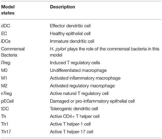
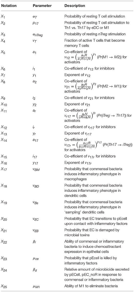
Table 2. System input parameters (adapted from [1]).

H. pylori is mainly found in the mucus layer lining the epithelial cells, and a small fraction is present in the lamina propria (LP). The immune cells participating in the immune response to H. pylori infection, including the T cells and macrophages, are found in the LP. The immune cells in the gastric lymph nodes (GLN) also play an important role in response to infection. As a proof of concept, in this study, we focus on the three types of macrophages M1 (classically activated, prone to promote inflammation), M2 (alternatively activated with regulatory, and pro-resolutory functions) and M0 (precursor of M1 and M2 macrophages) in the LP as the output variables. Figure 1 shows the state transition describing interactions among macrophages in Lamina Propria. The reader is referred to Bisset et al. [49] and Wendeldorf et al. [66] for details on the state transition functions for the remaining cell types. We denote these three outputs as M1_LP, M2_LP, and M0_LP respectively; see Table 3 for a brief description.

FIGURE 1

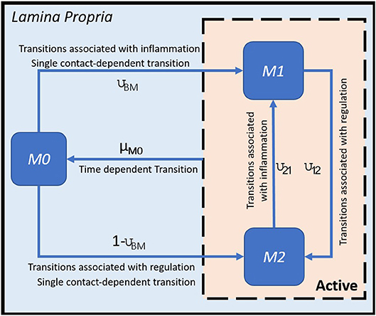
Figure 1. State transition functions for macrophages (adapted from [49]).

TABLE 3

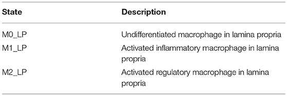
Table 3. Simulation output variables of interest.

The ENISI-based model of H. pylori is unique in the sense that it incorporates regulatory mechanisms of both adaptive and innate immunity, multi-location cell migration as well as cross talk between various cell types. In addition, this modeling framework is designed to represent each participating cell of the immune pathway which facilitates mapping of the model parameters to experimentally-driven predictions and therefore provides solid translational utility.

The ENISI-based model of H. pylori can be viewed as an extension of an agent-based model as it incorporates a procedural and interactive view of the underlying systems where components of the system interact locally with each other and the behavior of individual objects is described procedurally as a function of the internal state and the local interactions. This approach allows incorporation of both spatial effects and randomness of cell-cell and cell-bacteria contact. Furthermore, in the case of colonic inflammation spawned by a small number of pathogens, this randomness can significantly affect the outcome of the system as we have previously described [49]. However, scalability due to limitation of computational power is the main drawback of using this approach. The goal of the present work is to address this limitation by providing venues to draw conclusions based on multi-resolution SA where the number of simulation runs required to generate plausible hypotheses can be reduced and the simulation experiment can be better designed based on experts' prior knowledge.

In our previous work, we performed an ANOVA-based sensitivity analysis for the ENISI-based model of H. pylori infection [1]. The simulation model has the 25 input parameters listed in Table 2 (respectively denoted by X₁, X₂, …, X₂₅); and the value of each input parameter is assumed to vary among 4 different levels [1]. A full factorial design containing all possible combinations of the respective 4 levels of all 25 factors requires 4²⁵ = 1.126 × 10¹⁵ experiment runs; moreover, each simulation replication performed at a given input parameter combination takes about 90 min to execute. It is therefore impractical to perform simulation runs at all input parameter combinations specified by the full factorial design. As a remedy, we adopted an orthogonal array of 128 distinct combinations of the 25 input parameters with strength 2 [1]; let us denote the resulting 128 × 25 design matrix by ${D}$. Such a design has the following desirable properties: (i) projecting the input combinations onto any input dimension, there are 16 replications for each level; (ii) projecting the input combinations onto any two input dimensions (i.e., any two columns of ${D}$), it is a full factorial (4 × 4) with 8 replications for each level combination; (iii) projecting the input combinations onto a three-dimension subspace (labeled as X₁, X₂, and X₃), the projected points contain a full factorial design in any two-dimensional space of (X₁, X₂), (X₁, X₃), and (X₂, X₃). Therefore, the 128 distinct input combinations specified by ${D}$ are spread out in a 25-dimensional input parameter space; and simulation experiments are only required to be performed with these 128 combinations of input parameter levels. As the simulation outputs tend to be highly variable, replicated simulations are required at each input parameter combination to assess the uncertainty exhibited by each output of interest. We used 15 replications when simulating at each of the 128 input parameter combinations [1]. As a result, the resulting dataset contains outputs generated from a total number of 128 × 15 = 1, 920 simulation replications, with which sensitivity analysis was performed. As it is computationally prohibitive to perform simulation-based sensitivity analysis using ENISI, we consider developing a two-stage metamodel-based SA procedure to analyze the existing dataset from Alam et al. [1] for the purpose of studying the time-varying impact of each input parameter.

3. Two-Stage Metamodel-Based Sampling Design and Sensitivity Analysis

In this section, we first describe the sampling design for constructing the two-stage metamodels, then we provide details on the metamodel-based sensitivity analysis.

3.1. Sampling Design for the Two-Stage Metamodel Construction

In this subsection, we provide details on how to construct the two-stage metamodels with an increased temporal resolution using the existing dataset that we have previously created [1]. Besides the details given in section 2.3 about the experimental design and the resulting dataset, we note that for the sample path generated by each simulation replication run at a given input combination, four observations of each output variable are made per day; this amounts to 28 observations made per week and therefore 250 observations made over a 9-week period (all the time units are given in terms of equivalent lab experiment days). That is, each simulation replication at a given input parameter combination generates 250 observations of an output variable at 250 time steps.

In the first stage, we divide the entire dataset into three smaller datasets corresponding to the three time periods T₁, T₂, and T₃ as shown in Table 2, and we construct the first-stage metamodel using the three smaller datasets. In the second stage, we focus on investigating the T₂ period by dividing its corresponding dataset further into ten subsets in accordance with ten time segments as shown in Table 2. Such a study of the second stage will help investigate the time-varying impact of input parameters in a higher resolution, which enables us to focus on the peak of infection, occurring around week 3 post-infection [67].

Specifically, in the first stage, we group the observations of each output variable into three time periods, i.e., period 1 (T₁) consisting of week 1, period 2 (T₂) consisting of weeks 2–6, and period 3 (T₃) consisting of weeks 7–9, see Figure 2 for details. The sampling design we use for constructing the first-stage metamodel for a given output variable is obtained by crossing the original orthogonal array ${D}$ with the time-period index set ${{T}}_1=\left\{1,2,3\right\}$; hence, the resulting design includes 128 × 3 distinct design points, with its ith design point given by ${\text{w}}_i^{(1)}={({\text{X}}_i^{\top },t_i^{(1)})}^{\top }\in {D}\times {{T}}_1$ for i = 1, 2, …, 384; we obtain the corresponding point estimate of a given output variable at design point ${\text{w}}_i^{(1)}$, $\stackrel{-}{{Y}}({\text{w}}_i^{(1)})$, by averaging the observations collected at all time steps included in the time period indicated by $t_i^{(1)}$.

FIGURE 2

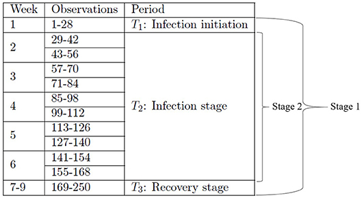
Figure 2. Time segments for the first- and second-stage analyses.

The second-stage analysis focuses on the T₂ period, i.e., weeks 2–6. We group the observations of each output variable in this period into 10 shorter segments, i.e., observations #29–42, #43–56, #57–70, #71–84, #85–98, #99–112, #113–126, #127–140, #141–154, and #155–168; see Figure 2 for details. The sampling design we use for constructing the second-stage metamodel for a given output variable is obtained by crossing the original orthogonal array ${D}$ with the time-segment index set ${{T}}_2=\left\{1,2,\dots ,10\right\}$. The resulting design therefore includes 128 × 10 distinct design points, with its ith point given by ${\text{w}}_i^{(2)}={({\text{X}}_i^{\top },t_i^{(2)})}^{\top }\in {D}\times {{T}}_2$, for i = 1, 2, …, 1, 280. As in the first stage, we obtain the corresponding point estimate of a given output variable at design point w_i, $\stackrel{-}{{Y}}(w_i^{(2)})$, by averaging the observations collected at all time steps included in the time segment indicated by $t_i^{(2)}$.

With the resulting dataset obtained by regrouping observations according to the aforementioned first-stage (respectively, second-stage) sampling design, we can construct a first-stage (resp., second-stage) metamodel following section 2.1 for each of the three output variables of interest (i.e., M1_LP, M2_LP and M0_LP). As values of the outputs are in unit of cell counts, which range from zero to a few thousand, to facilitate the use of GPR modeling, we transformed the values of the outputs from $\stackrel{-}{{Y}}(w_i^{(1)})$ into $log(\stackrel{-}{{Y}}(w_i^{(1)})+1)$ prior to constructing the first-stage metamodel; a similar practice is adopted in the second-stage metamodel construction as well. The metamodel fitting was carried out using the R package mlegp [68].

The goodness of fit of the resulting first- and second-stage metamodels can be assessed via the normal quantile plots shown in Figure 3; see more details from Figures S1, S2 in the Supplementary Material. We note that all plots shown in this paper involve cross-validated predictions and/or cross-validated standardized residuals. Using cross-validation means that for predictions made at a design point w, all observations at w are removed from the training set. In brief, we remark that the first-stage metamodels constructed for outputs M1_LP and M2_LP are more adequate as compared to those constructed for the other cases; a more detailed discussion on the metamodel fitting is provided in section 5. It is worth noting, however, that the simulated dataset we used were obtained according to the experimental design intended for an earlier study [1]; hence, though the metamodel fitting using this existing dataset does not appear ideal, we expect that the fit could be further improved by expanding the dataset using a more dedicated experimental design.

FIGURE 3

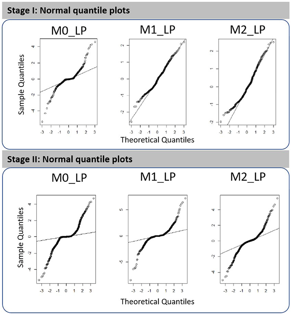
Figure 3. Normal quantile plots obtained for the fitted metamodels with respect to outputs M0_LP, M1_LP, and M2_LP in the first stage analysis (three time periods, i.e., T₁, T₂, and T₃) and in the second stage high-resolution analysis (10 time segments in T₂).

It is worthwhile explaining the rationale behind constructing the aforementioned two-stage metamodels and performing the subsequent sensitivity analysis. A more direct route may appear as to construct a single metamodel without binning the 250 time steps at all; yet this choice amounts to constructing a GP model using k = 128 × 250 = 32, 000 design points, a computationally intensive task itself as the computational time for training and prediction scales in ${O}(k^3)$, without taking into account the computational load due to sensitivity analysis yet. In contrast, with the first-stage analysis performed using the dataset in terms of three segments, we can construct a much more computationally efficient metamodel which facilitates sensitivity analysis to learn a rough trend of importance exhibited by the input parameters. This enables us to focus on the period to the domain experts' interest most and perform a more refined second-stage metamodel-based sensitivity analysis accordingly. We emphasize that our interest is in reusing an existing dataset to verify some conjectures and/or propose new hypotheses for the next rounds of experiments to test, hence the key is to develop an adaptive approach to exploit the dataset as much as possible, while striking a good balance between statistical and computational efficiency achieved.

3.2. Metamodel-Based Spatio-Temporal Sensitivity Analysis

Upon obtaining the first- and second-stage GPR models, we apply the Monte Carlo estimators of the first-order and total Sobol' indices proposed in Saltelli et al. [38] for metamodel-based sensitivity analysis. A summary of the notation used in this section is presented in Table 4.

TABLE 4

Table 4. Notation used for estimating Sobol' indices.

Following [38], we first generate three independent N × 25 sampling matrices A, B, and C from the 25-dimensional input parameter space via Latin hypercube sampling, each of which contains N distinct input combinations specified by their respective row; in our implementation N = 10, 000 is used. Then the predicted values were obtained using the input combinations specified by the rows of A and B and the GPR models fitted. We then estimate the total variance of a given output variable by the following estimator:

$\begin{array}{ll}\widehat{\text{Var}}(\hat{\text{Y}}(\text{C},t))=\frac{1}{N}{\displaystyle \sum _{w=1}^N}(\hat{\text{Y}}{({\text{C}}_w,t)}^2)-{\left(\frac{1}{N}{\displaystyle \sum _{w=1}^N}\hat{\text{Y}}({\text{C}}_w,t)\right)}^2,& (10)\end{array}$

where $\hat{\text{Y}}({\text{C}}_w,t)$ denotes the predicted value at the prediction point (C_w, t) using the first-stage (respectively, second-stage) GPR model following (4), with C_w representing the input combination specified by the wth row of matrix C and t ∈ {1, 2, 3} denoting the three time periods (resp., t ∈ {1, 2, …, 10} denoting the ten time segments in the second period).

The estimated variance-based first-order effect for the ith input parameter for i = 1, 2, …, 25 can be given as

$\begin{array}{l}{\widehat{V}}_i\left({\text{E}}_{~i}\left(\widehat{\text{Y}}(\text{C},t)|X_i\right)\right)=\widehat{\text{Var}}(\widehat{\text{Y}}(\text{C},t))\\ -\frac{1}{2N}{\displaystyle \sum _{w=1}^N{\left(\widehat{\text{Y}}({\text{B}}_w,t)-\widehat{\text{Y}}({({\text{A}}_{\text{B}}^{(i)})}_w,t)\right)}^2},& (11)\end{array}$

where $\hat{\text{Y}}({\text{B}}_w,t)$ and $\hat{\text{Y}}({({\text{A}}_{\text{B}}^{(i)})}_w,t)$ are as similarly defined as $\hat{\text{Y}}({\text{C}}_w,t)$, with ${\text{A}}_{\text{B}}^{(i)}$ denoting the N × 25 matrix whose ith column comes from matrix B and all the remaining columns are the same as matrix A's; and B_w and ${({\text{A}}_{\text{B}}^{(i)})}_w$ are as similarly defined as C_w. In fact, transforming from (B)_w into ${({\text{A}}_{\text{B}}^{(i)})}_w$ can be seen as a step in the direction along all the input parameters except for the ith one; see Figure 4 for an illustration.

FIGURE 4

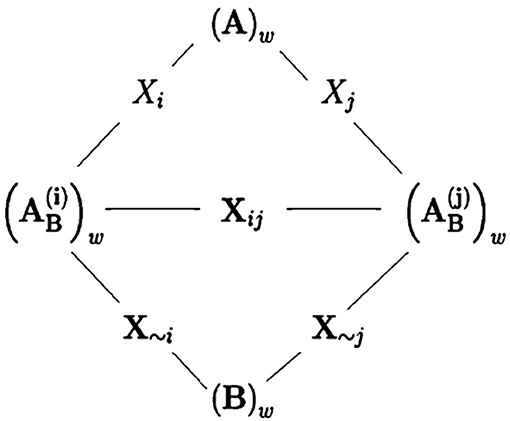
Figure 4. A figure by courtesy of Saltelli et al. [38] showing the relationships between sampling matrices. The wth row of matrix A and the wth row of of matrix $A_B^{(i)}$ are considered being separated by a step in the direction of X_i. Similarly, the wth row of matrix $A_B^{(i)}$ and the wth row of matrix B are considered separated by a step along the direction of X_~i. Finally, the wth row of matrix $A_B^{(i)}$ and the wth row of matrix $A_B^{(j)}$ are separated by a step along the direction of X_ij, i.e., the directions of both inputs X_i and X_j.

Finally, the estimated first-order Sobol' index for the ith input parameter in tth time period with t ∈ {1, 2, 3} (respectively, in the tth time segment of the second period with t ∈ {1, 2, …, 10}) can be obtained using the first-stage (resp., second-stage) GPR model as

$\begin{array}{ll}{\hat{S}}_i(X_i,t)=\frac{{\hat{V}}_i\left({\text{E}}_{~i}(\hat{\text{Y}}(\text{C},t)|X_i)\right)}{\widehat{\text{Var}}(\hat{\text{Y}}(\text{C},t))},i=1,2,\dots ,25.& (12)\end{array}$

In addition, we can obtain the estimated total sensitivity index for the ith input parameter in tth time period with t ∈ {1, 2, 3} (respectively, in the tth time segment of the second period with t ∈ {1, 2, …, 10}) using the first-stage (resp., second-stage) GPR model as

$\begin{array}{ll}{\hat{S}}_T(X_i,t)=\frac{{\hat{\text{E}}}_{~i}\left({\hat{V}}_i(\hat{\text{Y}}(\text{C},t)|X_{~i})\right)}{\widehat{\text{Var}}(\hat{\text{Y}}(\text{C},t))},i=1,2,\dots ,25,& (13)\end{array}$

where

$\begin{array}{ll}{\widehat{\text{E}}}_{~i}\left({\widehat{V}}_i(\widehat{\text{Y}}(\text{C},t)|X_{~i})\right)=\frac{1}{2N}{\displaystyle \sum _{w=1}^N{\left(\widehat{\text{Y}}({\text{A}}_w,t)-\widehat{\text{Y}}({({\text{A}}_{\text{B}}^{(i)})}_w,t)\right)}^2}.& (14)\end{array}$

4. Results

We first provide a detailed discussion on the multi-resolution sensitivity analysis results obtained by the two-stage metamodel-based procedure in section 4.1, then we compare these results with those obtained by the PRCC method in section 4.2.

4.1. Results Obtained by the Two-Stage Metamodel-Based Procedure

The resulting estimates of the Sobol' total indices for the 25 input parameters with respect to each output in periods 1 to 3 (T₁, T₂ with ten time segments, and T₃) are shown in Figure 5. We summarize the observations as follows.

FIGURE 5

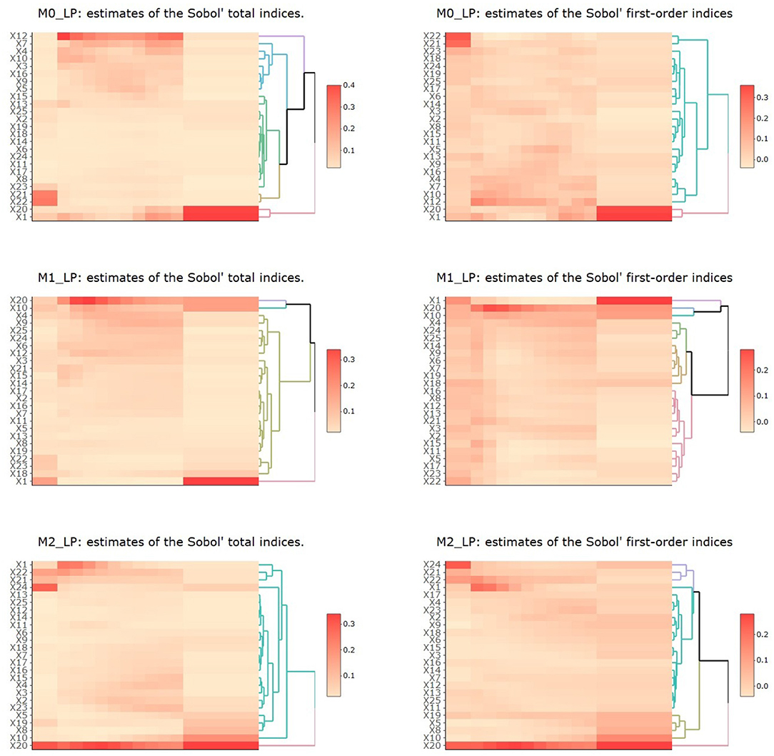
Figure 5. Heatmaps of estimates of Sobol' total and first-order indices for the 25 input parameters with respect to outputs M0_LP, M1_LP, and M2_LP. In each plot, the vertical axis denotes the 25 inputs and the horizontal axis denotes the three time periods T₁ to T₃, with T₂ being further divided into 10 time segments.

First, for M0_LP, the precursor of M1 and M2 macrophages in the LP, we observe that in the T₁ period, only X₂₁, X₂₂, which are related to the initiation of infection, had the most impact on M0_LP. As time progressed, X₁ and X₂₀ gradually became the most important input parameters (these parameters are related to the response to infection), whereas X₂₁, X₂₂ became less and less important. In the T₂ period with ten time segments, X₁₂ had the most impact, and the importance of X₇, X₄, X₂₀, and X₁ largely increased as time proceeded. During the early T₂ period, we observe the first wave of activities, including an increase in activated inflammatory macrophages M2 → M1, through parameter X₁₀ which diminishes as the time progresses during the peak of infection. During the same T₂ period, we also observe a second phase of activities, which were low and steadily increased over this period, including a shift from M1 to M2 (through parameters X₇, X₅, and X₉), and an increase in iTreg from Th17 (through parameter X₁₆). During the T₃ period, we observe an increase in pEcell and resting T cells simulations during the recovery stage, which started during the second half of the T₂ period. These observations are aligned with our understanding of the model dynamics and interacting entities in the model.

Second, for M1_LP, classically activated macrophages that are prone to promote inflammation, we observe that X₁ had the most impact in all three time periods, which indicates the importance of resting T cells. The parameter X₁₀ seemed to be higher during the peak of infection (around week 3), followed by the recovery stage, which indicates a higher probability of M1 → M2, a transition that is aligned with recovery and increase in immune regulation. X₂₀ (v_EC) was observed at its highest level around week 3. We note that the importance of this specific parameter was observed in our earlier study [1] and it is interesting to observe this trend using a different approach to SA. In fact, the importance of this parameter increases over time during the second stage (infection stage) and peaks at third week post infection and stabilizes afterwards. In our previous work [1], we had observed that the importance of parameter v_EC peaks at third week as well which further corroborates our previous observation. Using metamodeling approach, we observe that the importance of parameter 20 peaks towards the end of week 2 and slowly decrease over time reaching a stable level towards the recovery stage. The peak of importance and stabilizing of the impact of v_EC is smoother when analyzing the results using total indices as compared to first order indices that is when accounting for possible interaction influence of input parameters. This further highlights the robustness of this observation and further corroborates on the findings indicating that a regulator of gastric epithelial cell differentiation and function which is increased after H. pylori infection can be critical for macrophage recruitment to the stomach LP early after H. pylori infection [1, 58, 67, 69].

Third, for M2_LP, an alternatively activated macrophage with regulatory and pro-resolutory functions, we observe that X₂₀ had the most impact for this cell type throughout the different stages. The parameter X₂₀ (v_EC) is generally important for both M1 and M2 cell types. In three independent studies, using metamodeling, ANOVA based SA [1] as well as using PRCC method, we see very similar trends in terms of the importance of the parameter v_EC (parameter 20, the probability that an epithelial cell transitions into a proinflammatory state) with respect to M2 macrophages. In all three cases, we observe that v_EC is a highly important parameter in the model. In our previous reported study we noted that the peak of importance is after week 2, using PRCC we find that the peak of importance is toward the end of week 2 (second time segment at week 2) while using metamodeling approach, we note that the peak of importance ranges from end of week 2 to week 3, slowly decreasing after week 3. These results suggest that PRCC and ANOVA based techniques are better aligned as we would expect, given their underlying assumption and their implementation. The metamodeling provides a more computationally expensive alternative that could have higher resolution with respect to interaction influence of other parameters. However, overall these SA approaches are reproducible with slight variation in observation. Further experimental validation will be needed to corroborate the temporal prediction of these models. The parameter X₂₂ captured the ability of commensal or inflammatory bacteria to induce chemoattractant expression in epithelial cells and its importance for the M2 macrophages was higher during the first phase of the infection (until week 3) and it slowly decreased as time progressed. There were also a number of parameters (X₁₅, X₄, X₃, X₂ and X₂₃) that became more significant during the second half of the T₂ period. For example, X₃ captured the stimulation of resting nTreg and it is expected to be more important during the initiation of the recovery stage. Overall, these findings capture the dynamics of the system and highlight the importance of model parameters during the various stages of immune response to H. pylori infection. This is highly valuable, as the importance of a given input parameter over time can help us identify key elements that are time sensitive and also facilitate the identification of key input parameters for complex dynamic systems, such as the time to recovery or the recovery duration among others.

4.2. Comparison With Results Obtained by the PRCC Method

In this subsection, by focusing on the second-stage dataset, we compare the SA results obtained by the PRCC and Sobol' index methods for the top five most important input parameters identified for M0_LP, M1_LP, and M2_LP. The comparison results are shown in Figure 6, and the full analysis is available in the Github repository.

FIGURE 6

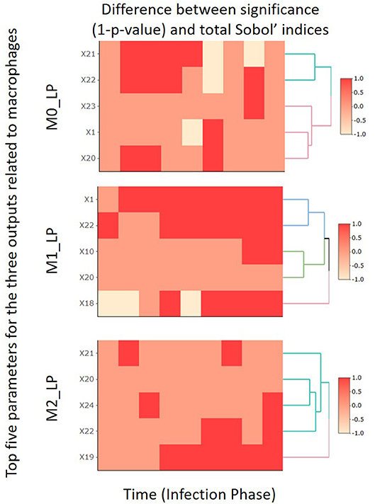
Figure 6. Comparison heatmaps of the PRCC and total indices obtained in the second-stage analysis focusing on the 10 time segments.

Specifically, we compare the change in the value of (1 − p) given by PRCC (p denotes the p-value obtained based on Equation 9) and that in the total Sobol' indices obtained by the Sobol' index method. We use “1” to label those cases where the two methods indicate a consistent trend (either increasing or decreasing) in the importance of a given input parameter, or cases where both methods report an absolute change in the level of importance that is smaller than 0.01. We use “−1” to label the cases where the two methods indicate inconsistent levels of importance, namely, one indicates an increasing trend yet the other indicates the opposite, or vice versa. Finally, the label “0” is used to denote those cases where one method reports an absolute change in the level of importance that is smaller than 0.01 whereas the other method reports an absolute change that is greater than 0.01.

For all three macrophages related outputs, we observe from Figure 6 that only a very small number of cases under consideration are labeled by “−1.” This indicates that the SA results given by the PRCC and Sobol' index methods are consistent in general; and this observation is especially true for the output M1_LP. It is worth noting that there are regions labeled with “0.” A closer examination of the corresponding cases reveals that the PRCC method tends to declare the input parameter under consideration significant while the Sobol' index method does not. This is consistent with the finding of Marino et al. [48] that the Sobol' index method tends to be more conservative as compared to the PRCC method; the Sobol' index method typically returns a smaller subset of input parameters with significant total index estimates when compared to the set of parameters with significant PRCC. We will provide further comments on these two methods in section 5.

5. Discussion

In this paper, we proposed a two-stage metamodel-based SA procedure to analyze the model of immune response to H. pylori infection. The first stage is based on three separate time periods (namely, infection initiation, infection stage and recovery stage), and the second stage focuses on ten time segments of the infection stage. Specifically, we fit the GPR models for each of the three outputs of interest (namely, M0_LP, M1_LP, and M2_LP) using the sampling matrix augmented with appropriate temporal index variables. We then obtain estimates of the Sobol' total and first-order indices for each input parameter using the fitted GPR models. These estimates of Sobol' indices enable us to efficiently quantify the time-varying significance of each parameter on each of the three system outputs of interest.

5.1. Pros and Cons of the PRCC and Sobol' Index Methods

In general, the PRCC method is a computationally efficient and reliable SA method in that it gives similar results as the Sobol' index method for a majority of the cases investigated. However, PRCC stipulates the restrictive assumption that a monotonic relationship exists between the output and each input parameter of interest, which is often violated by the underlying input-output relationship exhibited by the stochastic system of interest. Furthermore, as PRCC tends to return a larger set of input parameters identified as significant, it can lead to difficulty in identifying those few important input parameters from a large set [48]. The Sobol' index method, on the other hand, does not stipulate any restrictive assumption on the input-output relationship. Based on functional analysis of variance decomposition, it is able to apportion the variance of the output and quantify the effect of high-order interactions between input parameters. The Sobol' index method tends to produce relatively conservative SA results by returning a smaller set of important input paramters. In addition, the Sobol' index method is computationally more expensive than the PRCC method.

5.2. Strengths and Limitations

This study highlights the robustness and flexibility of our novel approach, as it was efficiently used in an experimental design and the resulting dataset that were created for an earlier SA study [1]. The fitting of the GPR models could be further improved with a larger training dataset dedicated to the proposed approach. The plots of observed vs. standardized residuals obtained for the fitted metamodels shown in Figure S2 indicate that the metamodel's fitting is better for M1_LP and M2_LP in the first-stage analysis as compared to the remaining cases. In particular, we observe some outliers in cross-validated predictions for M0_LP using the first- and second-stage GPR models constructed, and for M1_LP and M2_LP using the second-stage metamodels constructed. These findings again suggest that the original dataset may be too sparse to be used for building robust metamodels here. It is important to point out that given an existing dataset containing a fixed number of observations, the higher temporal resolution we look into, the less accurate the point estimates of an output variable we get; subsequently, the resulting higher-resolution spatio-temporal metamodel constructed based on these point estimates becomes less accurate.

It is valuable to emphasize that despite the lack of accuracy of some of the metamodels constructed, the SA results obtained using the proposed approach are aligned with those previously reported [1]. For instance, the trend of an important parameter X₂₀ (v_EC) observed here echoes the previously reported observations via a more traditional SA approach [1]; this provides a further support to the conclusion reached. Hence, given that the experimental design and the simulated dataset used here are not specifically intended for the metamodel-based SA approach, we argue that the SA results obtained seem reasonable and relevant, making the proposed approach adaptable to existing datasets. In brief, given an existing dataset to use, choosing an appropriate level of temporal resolution to perform a metamodel-based sensitivity analysis is a delicate issue. The two-stage procedure is proposed to proceed adaptively and has successfully confirmed the results by our earlier study [1].

5.3. Future Direction

For future research directions, we will explore the effect of time resolution for a given dataset and study the impact on the model outputs. This systematic analysis will help us better understand the limitations of our approach for sparser datasets, including situations where one is not able to generate more data (simulated or experimental). In addition, given customized designs and resulting datasets, we will conduct an in-depth study of interaction effects and higher-order effects associated with each input parameter under consideration. In particular, alternative SA methods will be considered, e.g., the sensitivity index maps method that examines the model behavior at each point of a spatio-temporal output domain, the block sensitivity indices method that summarizes the influence of the input parameters on the average value of the system output over a subset of the domain [70], and the generalized sensitivity analysis method that analyzes the influence of each input parameter over the entire output domain [45]. However, the aforementioned methods require collecting more data during each time period of interest. To the best of our knowledge, even with an adequate dataset available, the GPR modeling approach adopted in this paper can become too computationally expensive to apply for obtaining more refined spatio-temporal SA results. One potential way to address this challenge is to conduct functional principal component analysis (fPC) or proper orthogonal decomposition [71]. Each time-dependent output can be expanded in an appropriate functional coordinate system, and the metamodel-based generalized SA can be applied to the vector of fPC coefficients, such that the impact of each input parameter on the generation of different dynamic features exhibited by each system output of interest can be quantified efficiently. This research is currently underway.

5.4. Potential Applications

The metamodel-based SA approach can be applied to analyze other simulated stochastic systems, such as geologic computer models, as well as rich longitudinal datasets obtained from different fields, including financial, medical, literature, and social data sources. Examples of such sources include (1) social networks; (2) preclinical and clinical laboratory measures, to study health outcome and predict disease onset; (3) in silico clinical trials [72]; (4) electronic health records at large, which could link health information to socioeconomic status and physical activity as well as food environment; (5) wearable electronics (for monitoring health conditions or physical activities); and finally (6) unstructured text data from various sources including scientific literature. In all these cases, it is important to quantify the time-varying significance of a large number of parameters on the system outputs in a statistically and computationally efficient fashion.

Data Availability Statement

The datasets and the R code for this study can be found in the GitHub repository via the following link: https://github.com/wwvt/bioSA.

Author Contributions

All authors provided critical feedback and helped shape the research, analysis and manuscript. XC, VA, JB-R, and RH conceived the idea. VA and XC designed the experiments. XC, WW, and GX contributed to the code implementation and generating the results. VA, XC, AL, and MV analyzed and interpreted the results. XC, VA, WW, and GX prepared the figures and wrote the manuscript.

Funding

This work was supported by funds to XC from ICTAS Junior Faculty Award (No. 176371), the Nutritional Immunology and Molecular Medicine Laboratory (www.nimml.org), Geisinger Health System, as well as funds from the Defense Threat Reduction Agency (DTRA) to JB-R and RH (Virginia Tech, HDTRA1-18-1-0008), and to VA (Sub-PI, Geisinger, Subaward No. 450557-19D03). The funders had no role in study design, data collection, and interpretation, or the decision to submit the work for publication. The authors thank Virginia Tech Open Access Subvention Fund for supporting the publication of this work.

Conflict of Interest Statement

The authors declare that the research was conducted in the absence of any commercial or financial relationships that could be construed as a potential conflict of interest.

Supplementary Material

The Supplementary Material for this article can be found online at: https://www.frontiersin.org/articles/10.3389/fams.2019.00004/full#supplementary-material

References

1. Alam M, Deng X, Philipson C, Bassaganya-Riera J, Bisset K, Carbo A, et al. Sensitivity analysis of an ENteric Immunity SImulator (ENISI)-based model of immune responses to Helicobacter pylori infection. PLoS ONE (2015) 10:e0136139. doi: 10.1371/journal.pone.0136139

PubMed Abstract | CrossRef Full Text | Google Scholar

2. Yaesoubi R, Roberts SD. Important factors in screening for colorectal cancer. In: Henderson SG, Biller B, Hsieh MH, Shortle J, Tew JD, Barton RR, editors. Proceedings of the 2007 Winter Simulation Conference. Institute of Electrical and Electronics Engineers, Inc. (2007). p. 1475–82.

Google Scholar

3. Wan H, Ankenman BE, Nelson BL. Controlled sequential bifurcation: a new factor-screening method for discrete-event simulation. Operat Res. (2006) 54:743–55. doi: 10.1287/opre.1060.0311

CrossRef Full Text | Google Scholar

4. Baroni G, Tarantola S. A General Probabilistic Framework for uncertainty and global sensitivity analysis of deterministic models: a hydrological case study. Environ Modell Softw. (2014) 51:26–34. doi: 10.1016/j.envsoft.2013.09.022

CrossRef Full Text | Google Scholar

5. Pianosi F, Beven K, Freer J, Hall JW, Rougier J, Stephenson DB, et al. Sensitivity analysis of environmental models: a systematic review with practical workflow. Environ Modell Softw. (2016) 79:214–32. doi: 10.1016/j.envsoft.2016.02.008

CrossRef Full Text | Google Scholar

6. Meedeniya I, Buhnova B, Aleti A, Grunske L. Reliability-driven deployment optimization for embedded systems. J Syst Softw. (2011) 84:835–46. doi: 10.1016/j.jss.2011.01.004

CrossRef Full Text | Google Scholar

7. Meedeniya I, Moser I, Aleti A, Grunske L. Architecture-based reliability evaluation under uncertainty. In: Proceedings of the Joint ACM SIGSOFT Conference–QoSA and ACM SIGSOFT Symposium–ISARCS on Quality of Software Architectures–QoSA and Architecting Critical Systems–ISARCS. Boulder, CO: ACM (2011). p. 85–94.

Google Scholar

8. Sanchez SM, Lucas TW, Sanchez PJ, Nannini CJ, Wan H. Designs for large-scale simulation experiments, with applications to defense and homeland security. In: Hinkelmann K, editor. Design and Analysis of Experiments: Special Designs and Applications, Vol. 3, Hoboken, NJ: John Wiley & Sons, Inc. (2012). p. 413–41.

9. Rasmussen CE, Williams CKI. Gaussian Processes for Machine Learning. Cambridge, MA: The MIT Press (2006).

Google Scholar

10. Cao N, Low KH, Dolan JM. Multi-robot informative path planning for active sensing of environmental phenomena: a tale of two algorithms. In: Proceedings of the 2013 International Conference on Autonomous Agents and Multi-Agent Systems. International Foundation for Autonomous Agents and Multiagent Systems. Saint Paul, MN: (2013). p. 7–14.

Google Scholar

11. Chen J, Low KH, Yao Y, Jaillet P. Gaussian process decentralized data fusion and active sensing for spatiotemporal traffic modeling and prediction in mobility-on-demand systems. IEEE Trans Automat Sci Eng. (2015) 12:901–21. doi: 10.1109/TASE.2015.2422852

CrossRef Full Text | Google Scholar

12. Nychka D, Bandyopadhyay S, Hammerling D, Lindgren F, Sain S. A multiresolution Gaussian process model for the analysis of large spatial datasets. J Computat Graph Stat. (2015) 24:579–99. doi: 10.1080/10618600.2014.914946

CrossRef Full Text | Google Scholar

13. Datta A, Banerjee S, Finley AO, Gelfand AE. Hierarchical nearest-neighbor Gaussian process models for large geostatistical datasets. J Am Stat Assoc. (2016) 111:800–12. doi: 10.1080/01621459.2015.1044091

PubMed Abstract | CrossRef Full Text | Google Scholar

14. Ankenman BE, Nelson BL, Staum J. Stochastic kriging for simulation metamodeling. Operat Res. (2010) 58:371–82. doi: 10.1287/opre.1090.0754

CrossRef Full Text | Google Scholar

15. Santner TJ, Williams BJ, Notz WI. The Design and Analysis of Computer Experiments. New York, NY: Springer (2003).

Google Scholar

16. Kleijnen JPC. Design and Analysis of Simulation Experiments. 2nd ed. New York, NY: Springer (2015).

Google Scholar

17. Chen X, Ankenman BE, Nelson BL. The effects of common random numbers on stochastic kriging metamodels. ACM Trans Model Comput Simul. (2012) 22:1–20. doi: 10.1145/2331140.2331142

CrossRef Full Text | Google Scholar

18. Chen X, Kim KK. Stochastic kriging with biased sample estimates. ACM Trans Model Comput Simul. (2014) 24:1–23. doi: 10.1145/2567893

CrossRef Full Text | Google Scholar

19. Borgonovo E, Plischke E. Sensitivity analysis: a review of recent advances. Eur J Operat Res. (2016) 248:869–87. doi: 10.1016/j.ejor.2015.06.032

CrossRef Full Text | Google Scholar

20. Fang KT, Li R, Sudjianto A. Design and Modeling for Computer Experiments. Boca Raton, FL: Chapman & Hall/CRC (2006).

Google Scholar

21. Helton JC, Johnson JD, Sallaberry CJ, Storlie CB. Survey of sampling-based methods for uncertainty and sensitivity analysis. Reliabil Eng Syst Saf. (2006) 91:1175–209. doi: 10.1016/j.ress.2005.11.017

CrossRef Full Text | Google Scholar

22. Iooss B, Lemaître P. A review on global sensitivity analysis methods. In: Dellino G, Meloni C, editors. Uncertainty Management in Simulation-Optimization of Complex Systems. Vol. 59. New York, NY: Springer (2015). p. 101–22.

Google Scholar

23. Saltelli A, Chan K, Scott EM. Sensitivity Analysis. New York NY: Wiley (2009).

Google Scholar

24. Makowski D, Naud C, Jeuffroy M, Barbottin A, Monod H. Global sensitivity analysis for calculating the contribution of genetic parameters to the variance of crop model prediction. Reliabil Eng Syst Saf. (2006) 91:1142–7. doi: 10.1016/j.ress.2005.11.015

CrossRef Full Text | Google Scholar

25. Lefebvre S, Roblin A, Varet S, Durand G. A methodological approach for statistical evaluation of aircraft infrared signature. Reliabil Eng Syst Saf. (2010) 95:484–93. doi: 10.1016/j.ress.2009.12.002

CrossRef Full Text | Google Scholar

26. Auder B, De Crecy A, Iooss B, Marques M. Screening and metamodeling of computer experiments with functional outputs. Application to thermal–hydraulic computations. Reliabil Eng Syst Saf. (2012) 107:122–31. doi: 10.1016/j.ress.2011.10.017

CrossRef Full Text | Google Scholar

27. Iooss B, Van Dorpe F, Devictor N. Response surfaces and sensitivity analyses for an environmental model of dose calculations. Reliabil Eng Syst Saf. (2006) 91:1241–51. doi: 10.1016/j.ress.2005.11.021

CrossRef Full Text | Google Scholar

28. Volkova E, Iooss B, Van Dorpe F. Global sensitivity analysis for a numerical model of radionuclide migration from the RRC “Kurchatov Institute” radwaste disposal site. Stochast Environ Res Risk Assess. (2008) 22:17–31. doi: 10.1007/s00477-006-0093-y

CrossRef Full Text | Google Scholar

29. Marrel A, Iooss B, Jullien M, Laurent B, Volkova E. Global sensitivity analysis for models with spatially dependent outputs. Environmetrics (2011) 22:383–97. doi: 10.1002/env.1071

CrossRef Full Text | Google Scholar

30. Homma T, Saltelli A. Importance measures in global sensitivity analysis of nonlinear models. Reliabil Eng Syst Saf. (1996) 52:1–17. doi: 10.1016/0951-8320(96)00002-6

CrossRef Full Text | Google Scholar

31. Sobol IM. Global sensitivity indices for nonlinear mathematical models and their Monte Carlo estimates. Math Comput Simul. (2001) 55:271–80. doi: 10.1016/S0378-4754(00)00270-6

CrossRef Full Text | Google Scholar

32. Sudret B. Global sensitivity analysis using polynomial chaos expansions. Reliabil Eng Syst Saf. (2008) 93:964–79. doi: 10.1016/j.ress.2007.04.002

CrossRef Full Text | Google Scholar

33. Cukier RI, Levine HB, Schuler KE. Nonlinear sensitivity analysis of multiparameter model systems. J Comput Phys. (1978) 26:1–42. doi: 10.1016/0021-9991(78)90097-9

CrossRef Full Text | Google Scholar

34. Reedijk CI. Sensitivity Analysis of Model Output: Performance of Various Local and Global Sensitivity Measures on Reliability Problems. Delft University of Technology (2000).

35. Jansen MJW. Analysis of variance designs for model output. Comput Phys Commun. (1999) 117:35–43. doi: 10.1016/S0010-4655(98)00154-4

CrossRef Full Text | Google Scholar

36. Morris MD, Moore LM, McKay MD. Using orthogonal arrays in the sensitivity analysis of computer models. Technometrics (2008) 50:205–15. doi: 10.1198/004017008000000208

CrossRef Full Text | Google Scholar

37. Saltelli A. Making best use of model evaluations to compute sensitivity indices. Comput Phys Commun. (2002) 145:280–97. doi: 10.1016/S0010-4655(02)00280-1

CrossRef Full Text | Google Scholar

38. Saltelli A, Annoni P, Azzini I, Campolongo F, Ratto M, Tarantola S. Variance based sensitivity analysis of model output. Design and estimator for the total sensitivity index. Comput Phys Commun. (2010) 181:259–70. doi: 10.1016/j.cpc.2009.09.018

CrossRef Full Text | Google Scholar

39. Veiga SD, Gamboa F. Efficient estimation of sensitivity indices. J Nonparametric Stat. (2013) 25:573–95. doi: 10.1080/10485252.2013.784762

CrossRef Full Text | Google Scholar

40. Marrel A, Bertrand I, Laurent B, Roustant O. Calculations of Sobol indices for the Gaussian process metamodel. Reliabil Eng Syst Saf. (2009) 94:742–51. doi: 10.1016/j.ress.2008.07.008

CrossRef Full Text | Google Scholar

41. Oakley JE, O'Hagan A. Probabilistic sensitivity analyis of complex models: a Bayesian approach. J R Stat Soc Ser B. (2004) 66:751–69. doi: 10.1111/j.1467-9868.2004.05304.x

CrossRef Full Text | Google Scholar

42. Storlie CB, Swiler LP, Helton JC, Sallaberry CJ. Implementation and evaluation of nonparametric regression procedures for sensitivity analysis of computationally demanding models. Comput Phys Commun. (2009) 94:1735–63. doi: 10.1016/j.ress.2009.05.007

CrossRef Full Text | Google Scholar

43. Campbell K, McKay MD, Williams BJ. Sensitivity analysis when model outputs are functions. Reliabil Eng Syst Saf. (2006) 91:1468–72. doi: 10.1016/j.ress.2005.11.049

CrossRef Full Text | Google Scholar

44. Lamboni M, Monod H, Makowski D. Multivariate sensitivity analysis to measure global contribution of input factors in dynamic models. Reliabil Eng Syst Saf. (2011) 96:450–9. doi: 10.1016/j.ress.2010.12.002

CrossRef Full Text | Google Scholar

45. Gamboa F, Janon A, Klein T, Lagnoux A Sensitivity analysis for multidimensional and functional outputs. Electron J Stat. (2014) 8:575–603. doi: 10.1214/14-EJS895

CrossRef Full Text | Google Scholar

46. Saltelli A, Marivoet J. Non-parametric statistics in sensitivity analysis for model output: a comparison of selected techniques. Reliabil Eng Syst Saf. (1990) 28:229–53. doi: 10.1016/0951-8320(90)90065-U

CrossRef Full Text | Google Scholar

47. Blower SM, Dowlatabadi H. Sensitivity and uncertainty analysis of complex models of disease transmission: an HIV model, as an example. Int Stat Rev. (1994) 62:229–43. doi: 10.2307/1403510

CrossRef Full Text | Google Scholar

48. Marino S, Hogue IB, Ray CJ, Kirschner DE. A methodology for performing global uncertainty and sensitivity analysis in systems biology. J Theor Biol. (2008) 254:178–96. doi: 10.1016/j.jtbi.2008.04.011

PubMed Abstract | CrossRef Full Text | Google Scholar

49. Bisset K, Alam M, Bassaganya-Riera J, Carbo A, Eubank S, Hontecillas R, et al. High-performance interaction-based simulation of gut immunopathologies with enteric immunity simulator (ENISI). In: IEEE 26th International Parallel & Distributed Processing Symposium (IPDPS). Shanghai: IEEE (2012). p. 48–59.

Google Scholar

50. Wendelsdorf KV, Alam M, Bassaganya-Riera J, Bisset K, Eubank S, Hontecillas R, et al. ENteric Immunity SImulator: a tool for in silico study of gastroenteric infections. IEEE Trans Nanobiosci. (2012) 11:273–88. doi: 10.1109/TNB.2012.2211891

PubMed Abstract | CrossRef Full Text | Google Scholar

51. Stolte M. Helicobacter pylori gastritis and gastric MALT-lymphoma. Lancet (1992) 339:745–6. doi: 10.1016/0140-6736(92)90645-

PubMed Abstract | CrossRef Full Text | Google Scholar

52. Sharma CM, Pernitzsch SR. Transcriptome complexity and riboregulation in the human pathogen Helicobacter pylori. Front Cell Infect Microbiol. (2012) 2:14. doi: 10.3389/fcimb.2012.00014

PubMed Abstract | CrossRef Full Text | Google Scholar

53. Suerbaum S, Michetti P. Helicobacter pylori infection. N Engl J Med. (2002) 347:1175–86. doi: 10.1056/NEJMra020542

PubMed Abstract | CrossRef Full Text | Google Scholar

54. Amieva MR, El-Omar EM. Host-bacterial interactions in Helicobacter pylori infection. Gastroenterology (2008) 134:306–23. doi: 10.1053/j.gastro.2007.11.009

PubMed Abstract | CrossRef Full Text | Google Scholar

55. Pacifico L, Anania C, Osborn JF, Ferraro F, Chiesa C. Consequences of Helicobacter pylori infection in children. World J Gastroenterol. (2010) 16:5181. doi: 10.3748/wjg.v16.i41.5181

PubMed Abstract | CrossRef Full Text | Google Scholar

56. Arnold IC, Dehzad N, Reuter S, Martin H, Becher B, Taube C, et al. Helicobacter pylori infection prevents allergic asthma in mouse models through the induction of regulatory T cells. J Clin. Invest. (2011) 121:3088–93. doi: 10.1172/JCI45041

PubMed Abstract | CrossRef Full Text | Google Scholar

57. Selgrad M, Bornschein J, Kandulski A, Hille C, Weigt J, Roessner A, et al. Helicobacter pylori but not gastrin is associated with the development of colonic neoplasms. Int J Cancer (2014) 135:1127–31. doi: 10.1002/ijc.28758

CrossRef Full Text | Google Scholar

58. Bassaganya-Riera J, Dominguez-Bello MG, Kronsteiner B, Carbo A, Lu P, Viladomiu M, et al. Helicobacter pylori colonization ameliorates glucose homeostasis in mice through a PPAR γ-dependent mechanism. PLoS ONE (2012) 7:e50069. doi: 10.1371/journal.pone.0050069

PubMed Abstract | CrossRef Full Text | Google Scholar

59. Cook KW, Crooks J, Hussain K, O'Brien K, Braitch M, Kareem H, et al. Helicobacter pylori infection reduces disease severity in an experimental model of multiple sclerosis. Front Microbiol. (2015) 6:52. doi: 10.3389/fmicb.2015.00052

PubMed Abstract | CrossRef Full Text | Google Scholar

60. Engler DB, Reuter S, van Wijck Y, Urban S, Kyburz A, Maxeiner J, et al. Effective treatment of allergic airway inflammation with Helicobacter pylori immunomodulators requires BATF3-dependent dendritic cells and IL-10. Proc Natl Acad Sci USA. (2014) 111:11810–15. doi: 10.1073/pnas.1410579111

PubMed Abstract | CrossRef Full Text | Google Scholar

61. Kronsteiner B, Bassaganya-Riera J, Philipson C, Viladomiu M, Carbo A, Abedi V, et al. Systems-wide analyses of mucosal immune responses to Helicobacter pylori at the interface between pathogenicity and symbiosis. Gut Microbes (2016) 7:3–21. doi: 10.1080/19490976.2015.1116673

PubMed Abstract | CrossRef Full Text | Google Scholar

62. Abedi V, Hontecillas R, Hoops S, Liles N, Carbo A, Lu P, et al. ENISI multiscale modeling of mucosal immune responses driven by high performance computing. In: 2015 IEEE International Conference on Bioinformatics and Biomedicine (BIBM). Washington, DC: IEEE (2015). p. 680–4.

Google Scholar

63. Mei Y, Carbo A, Hontecillas R, Hoops S, Liles N, Lu P, et al. ENISI MSM: a novel multi-scale modeling platform for computational immunology. In: 2014 IEEE International Conference on Bioinformatics and Biomedicine (BIBM). Belfast: IEEE (2014). p. 391–96.

Google Scholar

64. Mei Y, Abedi V, Carbo A, Zhang X, Lu P, Philipson C, et al. Multiscale modeling of mucosal immune responses. BMC Bioinform. (2015) 16:S2. doi: 10.1186/1471-2105-16-S12-S2

PubMed Abstract | CrossRef Full Text | Google Scholar

65. Mei Y, Carbo A, Hoops S, Hontecillas R, Bassaganya-Riera J. ENISI SDE: a new web-based tool for modeling stochastic processes. IEEE/ACM Trans Comput Biol Bioinform. (2015) 12:289–97. doi: 10.1109/TCBB.2014.2351823

PubMed Abstract | CrossRef Full Text | Google Scholar

66. Wendeldorf KV, Bassaganya-Riera J, Bisset K, Eubank S, Hontecillas R, Marathe M. Enteric immunity simulator: a tool for in silico study of gut immunopathologies. In: 2011 IEEE International Conference on Bioinformatics and Biomedicine (BIBM). IEEE (2011). p. 462–9.

Google Scholar

67. Viladomiu M, Bassaganya-Riera J, Tubau-Juni N, Kronsteiner B, Leber A, Philipson CW, et al. Cooperation of gastric mononuclear phagocytes with Helicobacter pylori during colonization. J Immunol. (2017) 198:3195–204. doi: 10.4049/jimmunol.1601902

PubMed Abstract | CrossRef Full Text | Google Scholar

68. Dancik GM. mlegp: Maximum Likelihood Estimates of Gaussian Processes; 2018. R package version 3.1.6. Available online at: https://CRAN.R-project.org/package=mlegp

69. Schumacher MA, Donnelly JM, Engevik AC, Xiao C, Yang L, Kenny S, et al. Gastric Sonic Hedgehog acts as a macrophage chemoattractant during the immune response to Helicobacter pylori. Gastroenterology (2012) 142:1150–9. doi: 10.1053/j.gastro.2012.01.029

PubMed Abstract | CrossRef Full Text | Google Scholar

70. Marrel A, Saint-Geours N, Lozzo MD. Sensitivity analysis of spatial and/or temporal phenomena. In: Ghanem R, Higdon D, Owhadi H, editors. Handbook of Uncertainty Quantification. Springer International Publishing (2016). p. 1–31.

Google Scholar

71. Marrel A, Perot N, Mottet C. Development of a surrogate model and sensitivity analysis for spatio-temporal numerical simulators. Stochast Environ Res Risk Assess. (2015) 29:959–74. doi: 10.1007/s00477-014-0927-y

CrossRef Full Text | Google Scholar

72. Zand R, Abedi V, Hontecillas R, Lu P, Noorbakhsh-Sabet N, Verma M, et al. Development of synthetic patient populations and in silico clinical trials. In: Bassaganya-Riera J, editor. Accelerated Path to Cures. Cham: Springer International Publishing (2018). p. 57–77.

Google Scholar