Phase Coherence Induced by Additive Gaussian and Non-gaussian Noise in Excitable Networks With Application to Burst Suppression-Like Brain Signals

1. Introduction

Noise is omnipresent in nature [1] playing a synergetic role in numerous organic and inorganic processes [2]. Random spatial and/or temporal fluctuations in neural systems are essential for brain function: noise is a key component of numerous neural processes, allowing brain networks to enrich their dynamical repertoire [3], enhancing sensory processing and detection in animals [4], improving signal-to-noise ratio [5], and even by sustaining cognitive brain functions [6].

Much insight about how noise shapes neural processes can be gained by studying how noise impacts non-linear dynamical systems, especially their oscillatory properties. In contrast to multiplicative noise, which reflect parametric fluctuations that are known to transform the stability of numerous systems [7, 8], additive noise describes fluctuations originating from unknown sources or external fluctuations from outside of the system. Previous studies of large-scale systems have provided multiple examples of additive noise-induced phase transitions [9–12]. Recent studies on the impact of additive noise on networks of simplified delayed non-linear oscillators have demonstrated that noise shapes non-linear network interactions, hence tuning its spectral features [13, 14]. However, most of these studies have focused on dynamics close to instability [15] or on dynamics in weakly coupled networks [16]. It remains poorly understood how strong noise impacts natural systems that are strongly connected and far from the stability threshold [8, 17, 18].

To extend these results and explore how strong additive noise impacts a more realistic network and its oscillatory properties, the present work considers a generic non-linear activation-inhibition network model built of excitable systems. In addition to neural systems [19], such networks have also been observed in enzymatic systems [20] and autocatalytic patterns in sand dunes and other inorganic patterns [21]. In contrast to previous studies, here the isolated excitable populations do not oscillate on their own, and oscillatory behavior results from collective interactions tuned by additive noise. We show how additive (independent identically distributed or iid) Gaussian and (independent non-identically distributed or non-iid) non-Gaussian network noise shape non-linear interactions in the model, specifically how it impacts its oscillatory dynamics. Both iid and non-iid noise induce transitions from non-coherent non-rhythmic states to coherent oscillating states. To describe the observed phase transitions, we derive analytically a deterministic order parameter equation [17] where additive noise transforms the dynamics through a novel noise-dependent non-linear response function. Using these results, we demonstrate and fully characterize coherence resonance-like behavior for varying iid noise and varying heterogeneity of non-iid noise. In order to gain the analytical results, we assume homogeneity of the networks, ergodicity in groups of neurons and statistical independence of connectivity weights and system dynamics. Taken together, our work provides convincing support for burst suppression [22] dynamics observed in the mammalian brain under anesthesia gathered through electroencephalography. Indeed, our model and analysis shows that a decrease in additive noise triggers a phase transition whose spectral signature provides a physiological support of phenomena seen experimentally.

2. Methods

The subsequent sections show the derivation of mean-field dynamics and random fluctuations about the mean fields. The mean-field dynamics is determined by additive noise properties.

2.1. The Model

The present work considers a system of two networks with non-linear activation-inhibition interactions. The networks under study exhibit random connections motivated by network models for associative memory in the brain [23, 24].

We consider two coupled homogeneous networks ${V}$ and ${W}$ of number N whose nodes obey

$\begin{array}{ll}\begin{array}{c}\widehat{L}{V}_n={\displaystyle \sum _{m=1}^N}{F}_{nm}{h}_1\left[V_m\right]-{\displaystyle \sum _{m=1}^N}{M}_{nm}{h}_2\left[W_m\right]\\ +I_0^{(1)}+{{\xi }_n}^{(1)}(t)\hfill \\ \widehat{L}{W}_n=-{\displaystyle \sum _{m=1}^N}{F}_{nm}{h}_2\left[W_m\right]+{\displaystyle \sum _{m=1}^N}{M}_{nm}{h}_1\left[V_m\right]\\ +I_0^{(2)}+{{\xi }_n}^{(2)}(t)\hfill \end{array}& (1)\end{array}$

for n = 1, …, N, $V_n\in {V},W_n\in {W}$ and the temporal operator $\widehat{L}=d/dt+\widehat{I}$, where $\widehat{I}$ is the unity operator. This model resembles the basic microscopic network model that yields the famous population model of Wilson and Cowan [25] and that can show oscillatory dynamics [26]. The network connectivity matrices F ∈ ℜ^N×N and M ∈ ℜ^N×N are random with matrix elements F_nm, M_nm ≥ 0. Since the network ${V}$ excites other cells and ${W}$ inhibits other cells, the network ${V}$ and ${W}$ is excitatory and inhibitory, respectively. Each network is homogeneous with

$\begin{array}{ll}{\displaystyle \sum _{m=1}^N}{F}_{nm}=F^0,{\displaystyle \sum _{m=1}^N}{M}_{nm}=M^0& (2)\end{array}$

for all n ∈ [1;N] and constants F⁰, M⁰ > 0. This is a realistic assumption that has been affirmed experimentally [27]. In the following examples, without contraining generality we choose Erdös-Rényi networks [28] for simplicity with connection probability c, mean degree Nc, and connection weights $F_{nm}=F^0/cN,M_{nm}=M^0/cN$. This means the network is not fully connected.

Local node dynamics is linear and the non-linear transfer functions h_1,2[U] mediate non-local interactions with h₁[U] = H₀H[U], H₀ > 0, h₂[U] = H[U], and the Heaviside function H[V] = 0 ∀V < 0, H[V] = 1 ∀V > 0, and H[0] = 1/2. The constant H₀ denotes the ratio of maximum firing rates between activation and inhibitory populations. The external inputs $I_0^{(1,2)}$ are constant in time and over the networks.

2.2. Additive Noise

Both populations in Equation (1) are subjected to additive noise ${{\xi }_n}^{(1,2)}$. However, we allow one population to be driven by iid noise (${W}$), while the other (${V}$) can be driven by either iid- or non-iid noise. Specifically, according to this, and given that the noise processes are independent in time and between nodes we have

$\begin{array}{ll}\begin{array}{c}\langle {\xi }_n^{(1)}(t)\rangle ={\bar{\xi }}_n^{(1)},\langle {\xi }_n^{(2)}(t)\rangle =0,\\ \langle {\xi }_n^{(1)}(t){\xi }_m^{(1)}(\tau )\rangle =D_n^{(1)}{\delta }_{nm}\delta (t-\tau ),\\ \langle {\xi }_n^{(2)}(t){\xi }_m^{(2)}(\tau )\rangle =D^{(2)}{\delta }_{nm}\delta (t-\tau ),\\ \langle {\xi }_n^{(1)}(t){\xi }_m^{(2)}(\tau )\rangle =0\hfill \end{array}& (3)\end{array}$

for all n,m = 1, …, N with mean values ${\bar{\xi }}_n^{(1)}$, noise intensities $D_n^{(1)},D^{(2)}$ and 〈·〉 denotes the ensemble average. We point out that all stochastic processes in network ${W}$ have zero mean and identical variance D⁽²⁾ and thus are independent and identically distributed (iid). In contrast, additive noise in network ${V}$ may be inhomogeneous over nodes with node-dependent mean and variance. This case involves a superposition of different Gaussian distributions in the network and the network noise is non-identically distributed and thus non-iid.

Specifically, each noise process in network ${V}$ belongs to a certain class ${{G}}_m,m=1,\dots ,M$ of M classes. Noise processes ${\xi }_n^{(1)}$ in a class ${{G}}_m$, i.e., $n\in {{G}}_m$, share their means ${\bar{\xi }}_m$ and variances D_m

$\begin{array}{ll}\begin{array}{c}{\bar{\xi }}_m={\bar{\xi }}_n^{(1)},n\in {{G}}_m,\\ D_m=D_n^{(1)},n\in {{G}}_m,\end{array}& (4)\end{array}$

while different classes may exhibit different means and variances.

To derive the probability density function $p_{{V}}(\xi )$ of the noise process over the network ${V}$ at a certain time instance we assume that the noise processes in each class ${{G}}_m$ are ergodic, i.e., all noise processes in each class are stationary and hence the ensemble average equals the average over nodes. Then the mean and variance of class ${{G}}_m$ is

$\begin{array}{ll}\begin{array}{c}\frac{1}{N_m}{\displaystyle \sum _{n\in {{G}}_m}}{\xi }_n^{(1)}={\bar{\xi }}_m\\ \frac{1}{N_m}{\displaystyle \sum _{n\in {{G}}_m}}{\left({\xi }_n^{(1)}-{\bar{\xi }}_m\right)}^2=D_m\end{array}& (5)\end{array}$

where N_m is the number of nodes in class ${{G}}_m$. For the network mean

$\begin{array}{l}\bar{\epsilon }=\frac{1}{N}{\displaystyle \sum _{n=1}^N}{\xi }_n^{(1)}\\ =\frac{1}{N}\left({\displaystyle \sum _{n\in {{G}}_1}}{\xi }^{(1)}+{\displaystyle \sum _{n\in {{G}}_2}}{\xi }^{(1)}+\cdots +{\displaystyle \sum _{n\in {{G}}_M}}{\xi }^{(1)}\right)\hfill \\ =\frac{1}{N_1}\frac{N_1}{N}{\displaystyle \sum _{n\in {{G}}_1}}{\xi }^{(1)}+\cdots +\frac{1}{N_M}\frac{N_M}{N}{\displaystyle \sum _{n\in {{G}}_M}}{\xi }^{(1)}\hfill \\ ={\displaystyle \sum _{m=1}^M}{p}_m\frac{1}{N_m}{\displaystyle \sum _{n\in {{G}}_m}}{\xi }_n^{(1)}\hfill \\ ={\displaystyle \sum _{m=1}^M}{p}_m{\bar{\xi }}_m\hfill & (6)\end{array}$

with the constant weights p_m = N_m/N. Similarly

$\begin{array}{l}\bar{D}=\frac{1}{N}{\displaystyle \sum _{n=1}^N}{\left({\xi }_n^{(1)}-\bar{\epsilon }\right)}^2\\ ={\displaystyle \sum _{m=1}^M}{p}_m(D_m+{\bar{\xi }}_m^2)-{\bar{\epsilon }}^2& (7)\end{array}$

utilizing (5) and (6). These expressions for network mean and network variance show sums over the mean and variances of the noise classes $\left\{{{G}}_m\right\}$. This indicates that the probability function of the network noise $p_{{V}}(\xi )$ is a function of the probability density functions of the single classes as well. Indeed, we find

$\begin{array}{ll}{p}_{{V}}(\xi )={\displaystyle \sum _{m=1}^M}{p}_m{N}({\bar{\xi }}_m,D_m)& (8)\end{array}$

with

$\begin{array}{c}{\displaystyle {\int }_{-\infty }^{\infty }}\xi p_{{V}}(\xi )d\xi =\bar{\epsilon }\\ {\displaystyle {\int }_{-\infty }^{\infty }}{(\xi -\bar{\epsilon })}^2{p}_{{V}}(\xi )d\xi =\bar{D}.\end{array}$

For completeness, we define the average of additive noise in network ${W}$ to $\sum _{n=1}^N{\xi }_n^{(2)}(t)/N={\bar{\epsilon }}_2$.

2.3. Mean-Field Dynamics

By virtue of the random network connectivity, no finite spatial scale is prominent and the system converges to the mean field solution. In addition the noiseless case $D_n^{(1,2)}=0$ stipulates a single constant stationary solution $V_n^0=I_0^{(1)}+F_0{H}_0-M_0,W_n^0=I_0^{(2)}-F_0-M_0{H}_0$. Consequently, we expect that a solution, that is constant over the network, describes the network dynamics. A mathematical proof of this assumption would exceed the current work and we refer the reader to forthcoming work. However, as will be seen in later sections, this assumption holds true in the network under study and permits to describe the network dynamics very well.

We choose the ansatz

$\begin{array}{ll}\begin{array}{c}{V}_n(t)=\bar{V}(t)+{\upsilon }_n(t)\\ W_n(t)=\bar{W}(t)+{\pi }_n(t),\end{array}& (9)\end{array}$

where $\bar{V},\bar{W}$ are the averages over the respective network activity and υ_n, π_n denote the deviations from the average activity,

$\begin{array}{l}\frac{1}{N}{\displaystyle \sum _{n=1}^N}{\upsilon }_n=\bar{\upsilon },\frac{1}{N}{\displaystyle \sum _{n=1}^N}{\pi }_n=\bar{\pi }\end{array}$

with the mean deviations $\bar{\upsilon },\bar{\pi }$. Taking the sum ${\sum }_{n=1}^N/N$ on both sides of Equation (1) we find

$\begin{array}{ll}\begin{array}{c}\widehat{L}\bar{V}=\frac{1}{N}{\displaystyle \sum _{n,m=1}^N}{F}_{nm}{H}_{0}H\left[\bar{V}+{\upsilon }_m\right]\\ -\frac{1}{N}{\displaystyle \sum _{n,m=1}^N}{M}_{nm}H\left[\bar{W}+{\pi }_m\right]\hfill \\ +I_0^{(1)}+e_1(t)\hfill \\ \widehat{L}\bar{W}=-\frac{1}{N}{\displaystyle \sum _{n,m=1}^N}{F}_{nm}H\left[\bar{W}+{\pi }_m\right]\\ +\frac{1}{N}{\displaystyle \sum _{n,m=1}^N}{M}_{nm}{H}_{0}H\left[\bar{V}+{\upsilon }_m\right]\hfill \\ +I_0^{(2)}+e_2(t).\hfill \end{array}& (10)\end{array}$

where $e_1(t)=\bar{\epsilon }(t)-\bar{\upsilon }(t)-d\bar{\upsilon }(t)/dt,e_2(t)={\bar{\epsilon }}_2(t)-\bar{\pi }(t)-d\bar{\pi }(t)/dt$. We point out that $\bar{\epsilon },{\bar{\epsilon }}_2,\bar{\upsilon }$, and $\bar{\pi }$ do vanish for N → ∞ due the statistical law of large numbers and do not vanish for finite-size networks. These values vary randomly in time and hence e_1,2(t) are random as well. In the following, we assume large networks with $\left|e_1(t)\right|\ll \left|I_0^{(1)}\right|,\left|e_2(t)\right|\ll \left|I_0^{(2)}\right|$, and hence e_1,2 are considered as small stochastic forces that do not affect the dynamics of the mean-fields.

Since F_nm and υ_m are independent random numbers

$\begin{array}{l}{\displaystyle \sum _{m=1}^N}{F}_{nm}H\left[\bar{V}(t)+{\upsilon }_m\right]\\ =N\left(\frac{1}{N}{\displaystyle \sum _{m=1}^N}{F}_{nm}H\left[\bar{V}(t)+{\upsilon }_m\right]\right)\\ \approx N\left(\frac{1}{N}{\displaystyle \sum _{m=1}^N}{F}_{nm}\right)\left(\frac{1}{N}{\displaystyle \sum _{m=1}^N}H\left[\bar{V}(t)+{\upsilon }_m\right]\right)& (11)\end{array}$

utilizing the statistical independence between connectivity and stochastic process

$\begin{array}{l}{E}_m\left[F_{nm}H(\bar{V}+{\upsilon }_m)\right]\\ =E_m\left[F_{nm}\right]E_m\left[H(\bar{V}+{\upsilon }_m)\right]& (12)\end{array}$

with the expectation value $E_m\left[X_m\right]\approx \sum _{m=1}^N{X}_m/N$. We point out that condition (12) holds for a large enough number of connected nodes, i.e., for large enough mean degree cN ruling out sparse networks.

Then condition (12) leads to

$\begin{array}{ll}{H}_0{\displaystyle \sum _{m=1}^N}{F}_{nm}H\left[\bar{V}(t)+{\upsilon }_m(t)\right]=F^0{S}_1(\bar{V}(t))& (13)\end{array}$

and

$\begin{array}{l}{S}_1(\bar{V}(t))=\frac{H_0}{N}{\displaystyle \sum _{m=1}^N}H\left[\bar{V}(t)+{\upsilon }_m\right]\\ =H_0{\displaystyle {\int }_{-\infty }^{\infty }}H\left[\bar{V}(t)+\upsilon \right]p_{{V}}(\upsilon ,t)d\upsilon \hfill \\ +\epsilon (\bar{V},t).\hfill & (14)\end{array}$

with the probability density function $p_{{V}}(\upsilon ,t)$ of the deviations υ at time t. The term ε represents the finite-size error of the integral. Equivalently

$\begin{array}{ll}{M}^0{S}_2(\bar{W}(t))={\displaystyle \sum _{m=1}^N}{M}_{nm}H\left[\bar{W}(t)+{\pi }_m(t)\right]& (15)\end{array}$

$\begin{array}{l}{S}_2(\bar{W}(t))={\displaystyle {\int }_{-\infty }^{\infty }}H\left[\bar{W}(t)+\pi \right]p_{{W}}(\pi ,t)d\pi \\ +\eta (\bar{W},t).& (16)\end{array}$

with the estimation error η and the probability density function $p_{{W}}(\pi ,t)$ of deviations π. This yields the evolution equations for the average activity

$\begin{array}{ll}\begin{array}{c}\widehat{L}\bar{V}=F{S}_1(\bar{V})-M{S}_2(\bar{W})+I_1\\ \widehat{L}\bar{W}=-F{S}_2(\bar{W})+M{S}_1(\bar{V})+I_2\end{array}& (17)\end{array}$

with $F={\sum }_{n=1}^N{F}^0/N=F^0,M={\sum }_{n=1}^N{M}^0/N=M^0$, and $I_{1,2}=I_0^{1,2}+e_{1,2}$.

Finally inserting Equations (17) and (9) into (1), one obtains

$\begin{array}{ll}\begin{array}{c}\widehat{L}{\upsilon }_n=H_0{\displaystyle \sum _{m=1}^N}{F}_{nm}H\left[\bar{V}+{\upsilon }_m\right]-F{S}_1(\bar{V})\\ -{\displaystyle \sum _{m=1}^N}{M}_{nm}H\left[\bar{W}+{\pi }_m\right]+M{S}_2(\bar{W})\hfill \\ +e_1(t)+{{\xi }_n}^{(1)}\hfill \\ \widehat{L}{\pi }_n=-{\displaystyle \sum _{m=1}^N}{F}_{nm}H\left[\bar{W}+{\pi }_m\right]+F{S}_2(\bar{W})\\ +H_0{\displaystyle \sum _{m=1}^N}{M}_{nm}H\left[\bar{V}+{\upsilon }_m\right]-M{S}_1(\bar{V})\hfill \\ +e_2(t)+{{\xi }_n}^{(2)}.\hfill \end{array}& (18)\end{array}$

Utilizing Equations (13) and (15) yields the expressions in (18)

$\begin{array}{l}\begin{array}{c}{H}_0{\displaystyle \sum _{m=1}^N}{F}_{nm}H\left[\bar{V}+{\upsilon }_m\right]-F{S}_1(\bar{V})\\ =\left(F^0-\frac{1}{N}{\displaystyle \sum _{n=1}^N}{F}^0\right)S_1(\bar{V})\hfill \\ =0\hfill \\ {\displaystyle \sum _{m=1}^N}{M}_{nm}H\left[\bar{W}+{\pi }_m\right]-M{S}_2(\bar{W})\\ =\left(M^0-\frac{1}{N}{\displaystyle \sum _{n=1}^N}{M}^0\right)S_2(\bar{W})\hfill \\ =0\hfill \end{array}\end{array}$

Then the equivalent calculus for the remaining terms in Equations (18) yield for large networks (e_1,2(t) → 0)

$\begin{array}{ll}\begin{array}{c}\widehat{L}{\upsilon }_n={{\xi }_n}^{(1)}(t)\\ \widehat{L}{\pi }_n={{\xi }_n}^{(2)}(t).\end{array}& (19)\end{array}$

These equations describe Ornstein-Uhlenbeck processes and determine the probability density functions $p_{{V}}(\upsilon ,t)$ and $p_{{W}}(\pi ,t)$ [29].

Here, it is important to mention that the deviations υ_n, π_n decouple from the averages $\bar{V},\bar{W}$ and Equation (17) fully describe the non-linear dynamics of the system. This holds true only since the random variables {F_nm} and $\left\{H\left[\bar{V}+{\upsilon }_m\right]\right\}$ are statistically independent what is used in Equations (11) and (18). If this does not hold true, υ_n and π_n depend on $\bar{V},\bar{W}$ and Equation (17) are not sufficient to describe the system dynamics.

The evolution equations (17) depend on the probability density functions $p_{{V}}(\upsilon ,t),p_{{W}}(\pi ,t)$. For large times, the solutions of (19) are [29]

$\begin{array}{ll}{\upsilon }_n(t)={\displaystyle {\int }_{-\infty }^t}{e}^{-(t-\tau )}{\xi }_n^{(1)}(\tau )d\tau .& (20)\end{array}$

Utilizing the noise properties (3) we gain

$\begin{array}{c}\frac{1}{N_m}{\displaystyle \sum _{k\in {{G}}_m}}{\upsilon }_k(t)={\bar{\xi }}_m\\ \frac{1}{N_m}{\displaystyle \sum _{k\in {{G}}_m}}{({\upsilon }_k(t)-{\bar{\xi }}_m)}^2=D_m\end{array}$

and

$\begin{array}{lll}\frac{1}{N}{\displaystyle \sum _{k=1}^N}{\upsilon }_k(t)=\bar{\epsilon }& ,& \frac{1}{N}{\displaystyle \sum _{k=1}^N}{({\upsilon }_k(t)-\bar{\epsilon })}^2=\bar{D}\end{array}$

where ${\bar{\xi }}_m,D_m,\bar{\epsilon }$ and $\bar{D}$ are taken from Equations (5)–(7). Then the probability density function of network ${V}$ is

$\begin{array}{ll}{p}_{{V}}(\upsilon )={\displaystyle \sum _{m=1}^M}{p}_m{N}({\bar{\xi }}_m,D_m).& (21)\end{array}$

Additive noise in network ${W}$ is iid and hence $p_{{W}}(\pi )={N}(0,D^{(2)})$.

2.4. Power Spectrum

Power spectra of the average activities provide evidence on phase coherence in the interacting networks. To this end, we have computed numerically the power spectra of simulated activity $\bar{V}(t)$ by the Bartlett-Welch method with time window 100 s and overlap rate 0.995.

This numerical power spectrum involves the full non-linear dynamics of the system. To compute analytically the power spectrum of the average activity, we can approximate the non-linear dynamics by considering the stochastic system evolution about an equilibrium. To this end, we can write Equation (17) as

$\begin{array}{l}\frac{d\text{Z}}{dt}=\text{N}\left[\text{Z}\right]+\text{e}\end{array}$

with the state vector $\text{Z}=(\bar{V},\bar{W})$, the non-linear vector function N ∈ ℝ² and the noise term e = (e₁, e₂). Neglecting the noise, the equilibrium ${\text{Z}}_0=({\bar{V}}_0,{\bar{W}}_0)$ is defined by

$\begin{array}{l}{\bar{V}}_0=F{S}_1({\bar{V}}_0)-M{S}_2({\bar{W}}_0)+I_0^1\\ {\bar{W}}_0=-F{S}_2({\bar{W}}_0)+M{S}_1({\bar{V}}_0)+I_0^2.\end{array}$

Then small deviations from the equilibrium u = Z − Z₀ obeys du/dt = Lu + e with the linear matrix

$\begin{array}{ll}\text{L}=\left(\begin{array}{cc}-1+F{S}_1^{\prime }({\bar{V}}_0)& -M{S}_2^{\prime }({\bar{W}}_0)\\ M{S}_1^{\prime }({\bar{V}}_0)& -1-F{S}_2^{\prime }({\bar{W}}_0)\end{array}\right)& (22)\end{array}$

and the linear power spectrum of $\bar{V}(t)$ reads [30]

$\begin{array}{ll}R(\nu )=\frac{D_0(L_{22}^2+L_{12}^2+4{\pi }^2{\nu }^2)}{4{\pi }^2{(L_{11}+L_{22})}^2{\nu }^2+{(det\text{L}-4{\pi }^2{\nu }^2)}^2}& (23)\end{array}$

with frequency ν, the determinant detL and the matrix elements L_mn of L in (22). The terms $S_{1,2}^{\prime }(x)=d{S}_{1,2}/dx$ are the non-linear gains computed at the corresponding equilibrium. Since the noise e(t) results primarily from finite-size effects, its properties are hard to model. In Equation (23), we have assumed 〈e_1,2〉 = 0, 〈e_k(t)e_l(τ)〉 = D₀δ_klδ(t − τ) for simplicity. Consequently, the linear analytical power spectrum (23) does not include all non-linear stochastic effects and does not capture the correct noise strength, but it conveys a good approximation of the numerical power spectra while involving the additive noise-induced shaping of the non-linear interactions.

2.5. Phase Coherence and Bandpass Filter

The Phase Locking Value (PLV) has been developed by Lachaux et al. [31] and estimates the phase coherence between two signals s_1,2(t). The major idea is to compute the time-dependent phase, e.g., by wavelet transform, of each signal ϕ₁(f, t) and ϕ₂(f, t) in the frequency band about center frequency f at time t. This approach follows the idea of an instantaneous amplitude and phase of a signal (see e.g., [32–35] for more details). The implementation is based on the general idea of a linear filter

$\begin{array}{l}\tilde{s}(f,t)={\displaystyle {\int }_{-\infty }^{\infty }}s(\tau )w(f,t-\tau )d\tau ,\end{array}$

where a signal s(t) is filtered by a sliding window function w. This window exhibits an amplitude-modulated complex-valued oscillatory function with intrinsic frequency f. Heuristically, the phase of the filtered signal $\tilde{s}$ at time t and frequency f is the mean phase of the signal at time t with respect to the phase of the window function w.

Then one computes the circular variance (or PLV) in a time window of width w about each time instance t_n

$\begin{array}{l}{R}_{1,2}(f,t_n)=\frac{1}{w}{\displaystyle \sum _{s=-w/2}^{w/2}}|{cos}^2(\Delta \varphi (f,t_{n+s}))\\ +{sin}^2(\Delta \varphi (f,t_{n+s})){|}^2\end{array}$

with Δϕ(f, t_n) = ϕ₁(f, t_n) − ϕ₂(f, t_n). If R_1,2(f, t) = 1 both signals are maximum coherent in the frequency band about f at time t, R_1,2(f, t) = 0 indicates no phase coherence.

This is the classical bi-signal phase coherence. To obtain a measure for global phase coherence as considered in the present work, one may average the PLV of two signals s_n, s_m over a set of phase pairs ${M}$ of mass M [35] and gain the global Phase Locking Value

$\begin{array}{l}\text{gPLV}(f,t)=\frac{1}{M}{\displaystyle \sum _{n,m\in {M}}}{R}_{nm}(f,t),\end{array}$

that represents the degree of phase coherence in the system. Similar to the two-phase PLV, gPLV(f, t) = 1 reflects maximum phase coherence, i.e., all nodes in the system have identical phases, and gPLV(f, t) = 0 indicates that all nodes are out of phase.

In this context, it is important to note that instantaneous phase values are defined properly only in a certain time-frequency uncertainty interval for non-vanishing instantaneous amplitude in the same interval. To avoid spurious phase coherent values, we consider those phase pairs only, whose instantaneous spectral power exceeds 50% of the maximum spectral power at the corresponding time instance [36].

In the present work we determine phases by a Morlet wavelet transform [31] with center frequency f_c = 5, choose ${M}=\left\{n,m|n\in (1,250),m\in \left\{1,3,5,\dots ,499\right\}\right\}$, i.e., M = 498 pairs for phase pair averaging. Temporal averaging has been performed in the center of the time window with time points of number w = 3, 900.

Typical experimental electroencephalographic data (EEG) is bandpass filtered to remove artifacts and focus on certain frequency bands under study. To compare model solutions to experimental data, we apply a Butterworth-bandpass filter of 6th order with lower and higher cut-off frequency 1.25 and 50 Hz, respectively.

3. Results

This section presents the model topology for certain parameter sets and its dynamics for weak and strong noise, where the noise processes in the networks may be distributed uniformly (iid) or non-uniformly as a superposition of noise processes with different mean values (non-iid). The final application to brain activity indicates the possible importance of the stochastic analysis presented.

3.1. Additive iid-Noise

At first, we clarify the topology of Equation (17) providing first insight into the dynamics of the network dynamics. The subsequent numerical simulation of the full model (1) reveals a noise-induced phase transition from a non-coherent state to a phase-coherent state. The complementary analytical description explains this transition.

3.1.1. Equilibria and Linear Stability

The model system (1) exhibits diverse dynamics dependent of the matrices and the external input. From (17), we observe that the means of the network F⁰, M⁰, the maximum firing rate H₀, and the statistical properties of the external input fully determines the dynamics of the system. To achieve oscillatory activity, we have chosen parameters $F^0,M^0,I_2$ in such a way that bi-stable states may exist for some values of I₁, D₁, and D₂.

Since the additive noise processes $\left\{{\xi }_n^{(1)}\right\}$ are normally distributed, the probability density of υ_n at each node n in Equation (19) converges over time to the stationary normal distribution $p({\upsilon }_n)~{N}({\bar{\xi }}_n,D_1)$. For ${\bar{\xi }}_n=0$ all stationary fluctuations υ_n are iid and they obey the same probability density function leading to $p_{{V}}(\upsilon )~{N}(0,D_1)$ in Equation (14). This yields the transfer function (14)

$\begin{array}{l}{S}_1(\bar{V})={\displaystyle \underset{=S_0(\bar{V})}{{\displaystyle \underbrace{\frac{1}{2}\left[1-erf\left(-\frac{\bar{V}}{\sqrt{2D_1}}\right)\right]}}}}\\ +\epsilon (\bar{V}).& (24)\end{array}$

Figure 1 compares the theoretical transfer function and the numerical estimation in Equation (24) demonstrating very good accordance. In addition, one observes that larger additive noise level flattens the transfer function and hence affects the non-linear interactions in the system [37].

FIGURE 1

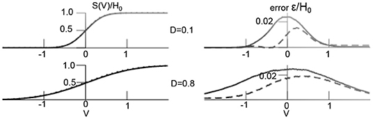
Figure 1. Additive noise shapes non-linear transfer function. (Left) Theoretical transfer function [integral in (24)] (dashed line) and numerical estimation of (24) averaged over 1,000 time points in simulation shown in Figure 4. (Right) distributions of difference between theoretical and numerical estimation ε (dashed line denotes temporal mean, solid line is temporal variance). Other parameters are D₂ = 0.5, H₀ = 1.7, results for the transfer function S₂ are equivalent.

The networks ${V}$ and ${W}$ excite and inhibit themselves (E − E and I − I interactions) described by the connectivity matrix F with strength F⁰. Their cross-interactions E − I and I − E are given by the matrix M with strength M⁰. In neuroscience, the balance between excitation and inhibition is supposed to play an important role in neural information processing [30, 38, 39]. In spatially extended biological systems, the balance between excitation and inhibition determines the type of emerging spatio-temporal patterns [40]. To obtain a first insight into the possible dynamics of the system (1), we define the ratio of excitation and inhibition γ = F⁰/M⁰.

Then the equilibrium $({\bar{V}}_0,{\bar{W}}_0)$ of Equation (17) with e_1,2 = 0 is gained by $d\bar{V}/dt=0,d\bar{W}/dt=0$. Utilizing Equation (24) and the equivalent formulation for transfer function S₂ and linearization of Equation (17) about the equilibrium the ansatz $(\bar{V}(t),\bar{W}(t))=\text{z}{e}^{\lambda t}$ with the eigenvector z allows to compute the Lyapunov exponents ${\lambda }_{1,2}\in {C}$. For complex-valued Lyapunov exponents, i.e., oscillation about the equilibrium, the imaginary part reads

$\begin{array}{ll}\text{Im}(\lambda )=\frac{\sqrt{4{\left(M^0\right)}^2{s}_1{s}_2-{\left(F^0\right)}^2{\left(s_1+s_2\right)}^2}}{2}& (25)\end{array}$

where s_1,2 = dS_1,2(x)/dx are the non-linear gains evaluated at the corresponding equilibrium. Then the eigenfrequency of the oscillation is f = Im(λ)/2π.

Figure 2 shows the equilibrium $({\bar{V}}_0,{\bar{W}}_0)$ as a function of the excitation–inhibition ratio γ. The linear stability of the equilibrium is read off the maximum real part of the Lyapunov exponent λ_max = max(Re(λ₁), Re(λ₂)). Increasing γ, the system exhibits a single stable focus at low values followed by bistability with top stable node, bottom stable focus, and a center saddle node. For larger γ, the lower stable focus loses stability and transitions to an unstable focus. This transition yields two unstable equilibria and a single top stable node. Further increase of γ causes center and bottom equilibrium to vanish while retaining the top stable node that does not change its stability for larger γ. The frequency of the bottom focus decreases monotonously with increasing γ.

FIGURE 2

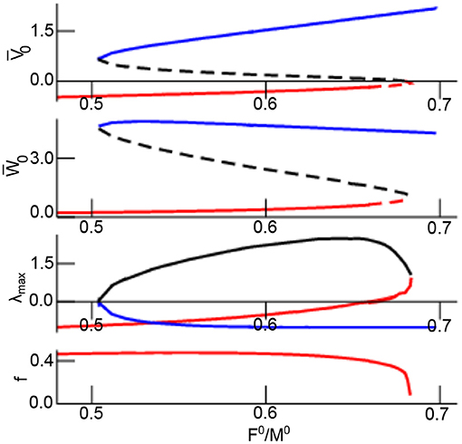
Figure 2. Equilibria ${\bar{V}}_0,{\bar{W}}_0$ and their stability as a function of γ = F⁰/M⁰. The top equilibrium is coded in blue line color, the center and bottom equilibrium is coded as black and red line in all panels. The lower panel shows the eigenfrequency of the bottom focus. The two top panels present stable equilibria by solid line and unstable equilibrium by dashed line. Further parameters are $M^0=3.87,H_0=1.7,I_1=1.45,I_2=0.4$ assuming iid-noise in both networks with $D_n^{(1)}=0.2,D^{(2)}=0.5$.

Decreasing the cross-network interaction strength M⁰ retains the bi-stability (Figure 3) and M⁰ → 0 but makes the lower focus and center node vanish yielding the single equilibrium ${\bar{V}}_0\to I_1,{\bar{W}}_0\to I_2$ (horizontal line in Figure 3). For large values ${\bar{V}}_0,{\bar{W}}_0$ the top stable node converges to

$\begin{array}{l}{\bar{V}}_0(\gamma )=M^0{H}_0\gamma -M^0+I_1\\ {\bar{W}}_0(\gamma )=-M^0\gamma +M^0{H}_0+I_2,\end{array}$

see dotted line in Figure 3. Then M⁰ → ∞ leads to a single equilibrium at γ = 1/H₀ (vertical dotted line in Figure 3). For M⁰ → ∞ but small values ${\bar{V}}_0,{\bar{W}}_0$, we obtain γ → 1 and $S_1({\bar{V}}_0)\to S_2({\bar{W}}_0)$, i.e., ${\bar{V}}_0\approx {\bar{W}}_0\approx 0$. Both latter cases for M⁰ → ∞ are illustrated in Figure 3: the larger the cross-interaction strength M⁰ the steeper the function ${\bar{V}}_0(\gamma )$ for large ${\bar{V}}_0,{\bar{W}}_0$ and the more the right-hand side bistability border stretches to the right. This analysis shows that, for the chosen constant external input and the given noise levels, the bistability between top stable node and bottom oscillatory node is present for γ ≤ 1, i.e., F⁰ ≤ M⁰. We point out that different external input may yield bistability for γ > 1 and refer to future work.

FIGURE 3

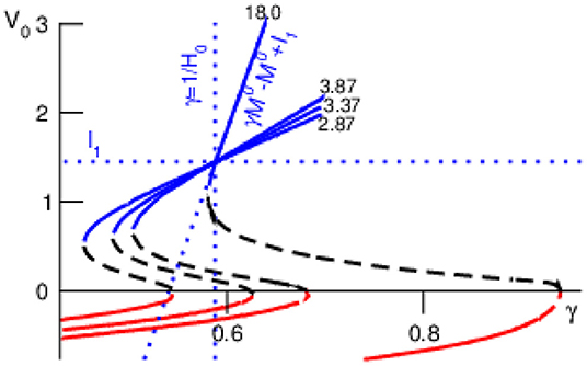
Figure 3. Equilibria of ${\bar{V}}_0$ and their stability for various values of M⁰ (numbers in plot). Other parameter values are taken from Figure 2.

3.1.2. Numerical Results and Analytical Explanation

Figure 4A (left hand side) shows solutions of Equation (1) for low noise levels fluctuating about the stationary solution V₀, cf. the time series of $\bar{V}(t)$ seen in Figure 4B (left hand side), and equivalently about W₀ (not shown). The stochastic stability of V₀, W₀ for low noise intensity agrees with the deterministic stability for $D_1,D^{(2)}=0$.

FIGURE 4

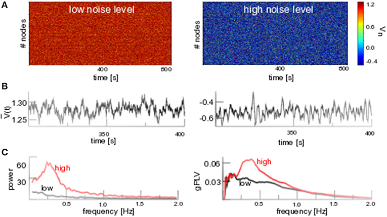
Figure 4. Additive noise induces phase coherent oscillations. (A) D₁ = 0.1 (low noise level) and D₁ = 0.8 (high noise level). (B) Temporal snapshot of spatial average $\bar{V}(t)=\sum _{n=1}^N{V}_n(t)/N$ for both noise levels. (C, left) Power spectrum of $\bar{V}$ for both noise levels. (C, right) Global phase coherence gPLV for both noise levels. Other parameters are $D_2=0.5,F^0=2.18,M^0=3.87,H_0=1.7,I_1=1.45,I_2=0.4,c=0.95,N=500,$ integration time step Δt = 0.1s with application of the Euler-Maryuama integration technique [41]. Results for W_n are equivalent.

In contrast, strong noise (D₁ = 0.8) yields a new lower equilibrium at $V_n^0<0,n=1,\dots ,N$ (cf. Figures 4A,B). New additive noise-induced states have been studied already close to stability thresholds [9, 11, 42] for small noise intensities, however not for large additive noise intensities far from stability thresholds that we address here. The new lower state exhibits an augmented spatio-temporal coherence that is observed both as a prominent spectral peak at f ≈ 0.3 Hz in the power spectrum of the spatial average $\bar{V}(t)$ and the prominent temporally averaged spatial coherence gPLV (cf. Figure 4C). Similar results are gained for networks with medium mean degree cN but not for low mean degrees (cf. the Appendix).

Additive noise triggers multistability in the network. Indeed, the analysis of equilibria of Equation (17) with e_1,2 = 0 reveals three states for low noise levels D₁ and a single state for large D₁ (cf. Figure 5). Linear stability analysis of the equilibria (cf. section 3.1.1), further reveals bistability with a stable node in the top branch, an unstable center node and a stable focus at the bottom equilibrium.

FIGURE 5

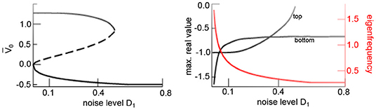
Figure 5. Additive noise induces bistability. Equilibria of (17) as a function to the noise level D₁ showing noise-induced hysteresis. (Left) Asymptotically stable (solid) and unstable states (dashed). (Right) Maximum real eigenvalues of stable states (black) and eigenfrequency of bottom equilibrium (red). Other parameters are taken from Figure 4. Results for W_n(t) are equivalent.

The eigenfrequency of the stable focus f diminishes with increasing noise level since the transfer function flattens and hence decreases s₁ (cf. Equation 25). The eigenfrequency approaches f ~ 0.3Hz for D₁ = 0.8 (cf. Figure 5) and agrees with the oscillation frequency of the spatial mean, shown in Figure 4. Summarizing, this analysis reveals that the transition from a top activity state to a bottom activity state with increasing noise level observed in Figure 4 is a phase transition from a stable node to a stable focus.

Figure 4B shows stochastically evolving spatial averages $\bar{V}$. The stochastic force originates from the error of the transfer function ε seen in Figure 1 (cf. Equation 24), and the finite-size correction terms e_1,2. Since ε and e_1,2 are random and vary over time, their sum represents a stochastic force in Equation (17).

3.2. Extension to Additive Non-iid Noise

We have seen above that the iid additive noise force shapes the non-linear interactions. Now we relax the condition of a vanishing noise average at each node and consider non-iid noise, i.e., a non-Gaussian probability density function $p_{{V}}(\upsilon )$. Equation (21) allows to describe heterogeneous non-iid noise, i.e., Gaussian processes with diverse means ${\bar{\xi }}_n^1$ and variances $D_n^{(1)}$. To demonstrate the effect of non-iid additive noise on our system, we consider M = 2 classes of Gaussian processes with identical variance and ${\bar{\xi }}_1=-{\bar{\xi }}_2=\Delta \mu ,p_{1,2}=0.5$ and distribute the additive noise processes of both classes uniformly over the network. Here Δμ is the noise mean shift and quantifies the degree of noise heterogeneity. Figure 6A presents the field activity V(t) where Δμ increases linearly in time. We observe a transition from an upper state to a lower state at Δμ ≈ 0.68. Similar to Figure 5, this phase transition involves a jump from a non-oscillatory non-coherent state to an oscillatory phase-coherent state (cf. Figures 6B,C). To understand this transition, we consider again the averages $\bar{V},\bar{W}$ and their temporal evolution according to Equation (17). Figures 6D,E show the corresponding equilibria and their linear stability subject to the noise mean shift. For weak noise heterogeneity, i.e., small Δμ, the system is bistable. Large heterogeneity transforms it to a monostable system with an oscillating state via a saddle-node bifurcation. The eigenfrequency of the oscillation state of f = 0.5Hz is close to the maximum power and phase coherence peak frequency of f ≈ 0.25 Hz in Figures 6B,C. This difference originates from the approximation error of the transfer functions S (cf. Figure 1), resulting to an effective increase in additive noise. For instance, increasing the additive noise variance to $D_1+0.02·H_0{F}^0$ (cf. Figure 1) decreases the eigen frequency at Δμ = 0.8 in Figure 6 to f = 0.3Hz, i.e., much closer to the observed value. Figure 6F (top panel) compares the analytical (Equation 8) and numerical solution of the probability density $p_{{V}}(\upsilon )$ for homogeneous and heterogeneous additive noise and confirms good agreement between the analysis and numerics. The corresponding transfer functions show good agreement as well (cf. Figure 6F, bottom panel).

FIGURE 6

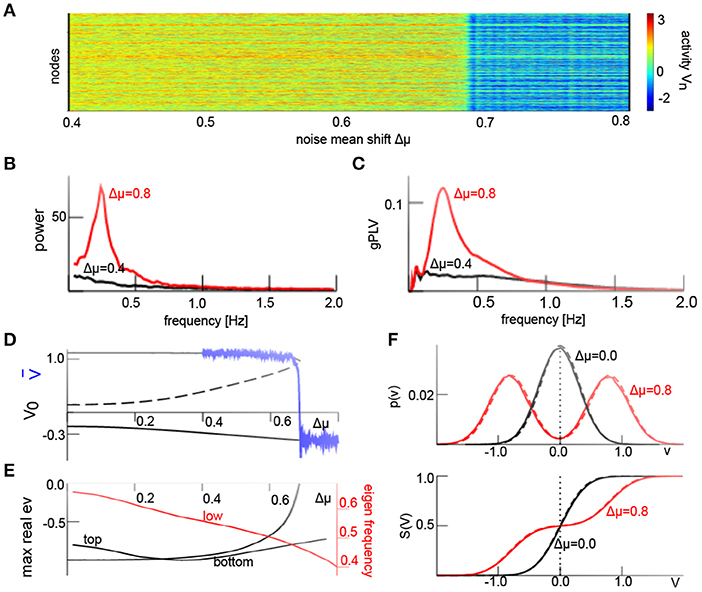
Figure 6. Additive non-iid noise induces phase coherent oscillations. (A) Spatio-temporal activity V(t) and jump from non-oscillatory high-activity to oscillatory low-activity state for increasing noise mean shift Δμ in the interval Δμ ∈ [0.4; 0.8] over 200s. (B) Power spectral density of spatial mean $\bar{V}(t)$ computed in a time window of 800s. (C) Global phase coherence gPLV in a time window of 400s. (D) Equilibria ${\bar{V}}_0$ (black) and simulated spatial average $\bar{V}(t)$, solid (dashed) lines denote stable (unstable) states. (E) Maximum Lyapunov exponents of respective stable equilibria (black) and eigenfrequency of the bottom state (red). (F) probability density function p(υ) (8) and resulting transfer functions (24) from analysis (solid line) and numerical solution (dashed line). D₁ = 0.1 and other parameters are taken from Figure 4; results for W_n(t) are equivalent. We have applied the Euler-Maryuama integration technique [41] with time step Δt = 0.1.

3.3. Link to Coherence Resonance

Coherence resonance is present when applied noise induces regular rhythms in a system, although the noise-free system does not [43–45]. We have investigated whether the noise-induced transition from non-rhythmic non-coherent system dynamics to rhythmic coherent dynamics shows this phenomenon over a larger range of noise intensities as well. Figure 7 (left) shows the power spectrum of $\bar{V}(t)$ subjected to additive iid-noise (cf. Figure 4). We observe no rhythmic activity for small noise intensity (the system evolves on the top branch seen in Figure 4), whereas coherent network activity is present for large noise D₁ ≥ 0.5. In comparison to the analysis shown in Figures 4–7 (left) shows a spectral peak that moves to lower frequencies for larger noise intensities while diminishing in power. Finally, for very large noise intensities D₁ > 10.5, the spectral peak vanishes. This means that coherent network activity is present for intermediate noise levels and the system does not exhibit coherent activity for very small and very large noise intensities. Qualitatively, this resembles coherence resonance.

FIGURE 7

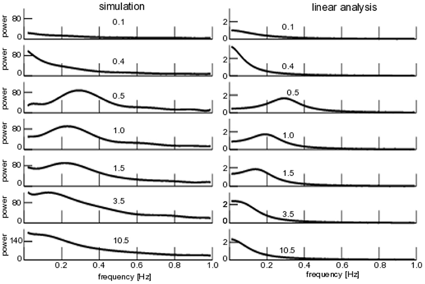
Figure 7. Power spectra of $\bar{V}(t)$ for additive iid noise. (Left) Numerical power spectra. (Right) Analytical power spectra according to Equation (23). The numbers give the noise intensity D₁, parameters are taken from Figure 4.

To evaluate our analytical description, Figure 7 (right) shows the linear power spectrum about the corresponding equilibrium and we observe a qualitatively similar power spectrum subject to the noise intensity, i.e., no phase coherence rhythmic state for very small and very large noise intensities but a spectral peak for intermediate levels. We point out that the analytical power spectrum reproduces quantitatively well the spectral peak frequency at low noise intensities, while the spectral peak already vanishes for noise intensities smaller than the ones observed in the numerical study.

To complete the study, Figure 8 compares the numerical and analytical power spectra similar to Figure 7, but now varying the degree of noise heterogeneity Δμ. We observe a coherence resonance-like behavior with a maximum coherence at intermediate levels of heterogeneity and vanishing coherence at very low and very high degrees of heterogeneity. Both numerical and analytical spectra are similar qualitatively, but differ in the frequency of maximum coherence. This results from the linear approximation of the analytical power spectrum and the finite-size effect observed and discussed already in the context of Figure 6.

FIGURE 8

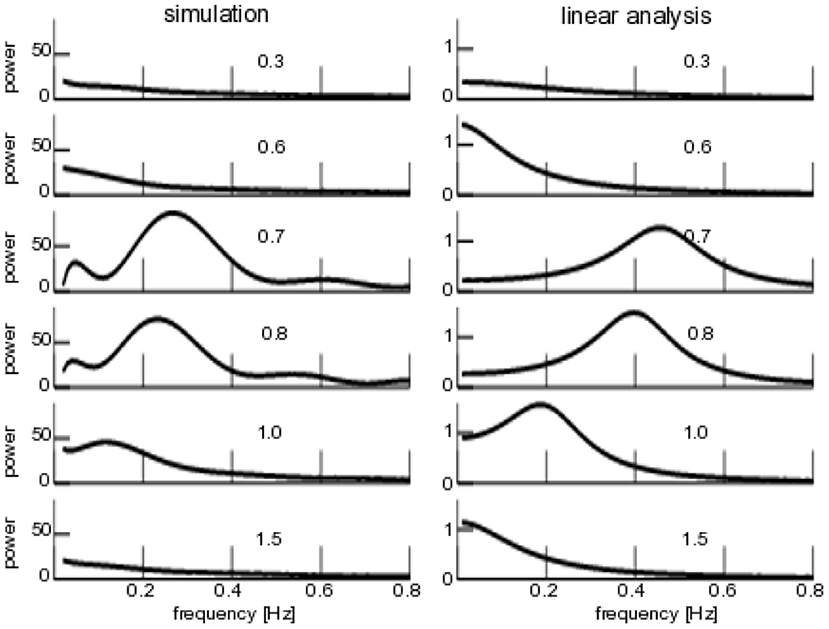
Figure 8. Power spectra of $\bar{V}(t)$ for additive non-iid noise. (Left) Numerical power spectra. (Right) Analytical power spectra according to Equation (23). The numbers give the degree of noise heterogeneity Δμ, noise intensity is D₁ = 0.1, other parameters are taken from Figure 6.

3.4. Experimental Results

Finally, to illustrate the importance of the demonstrated results, we consider experimental human brain data. An electroencephalogram (EEG) was recorded during isoflurane induced cardiac anesthesia from a polar FP1 to mastoid derivation at 125 Hz sampling rate using a Narcotrend (R) monitor (MT MonitorTechnik, Hannover, Germany). The EEG was recorded as part of the EPOCAS study (National Clinical Trials number 02976584). A bandpass filter from 0.5 to 45 Hz was applied and cardiac artifacts minimized by subtracting an artificial artifact reference signal from the EEG.

In Figure 9A the upper panel shows an episode with burst suppression, i.e., an intermittent suppression of high-amplitude to small-amplitude activity. Here, burst EEG shows a broad frequency band and the suppressed EEG exhibits oscillations in a narrow frequency band at about 8 Hz (lower panel). This burst suppression was caused experimentally by a rapid increase in isoflurane concentration from 0.8 to 1.8% (not shown). This jump from a broad frequency range activity to a coherent oscillation in a narrow frequency band resembles the additive noise effect described in the paragraphs above. The electromagnetic source of EEG lies in the cortex and the reticular activation system (RAS) in the brain sets the excitation level of the cortex [46]. We assume that model (1) describes cortical activity and the additive input is supposed to originate directly or indirectly from the RAS. Under anesthesia, RAS activity varies [47] and hence burst suppression may result from reduced RAS input induced by increased isoflurane concentration. Moreover, synaptic inhibition in local cortical structures may also decrease the intrinsic noise level [36, 48]. Hence D₁ reduces for larger isoflurane concentration. Figure 9B (upper panel) shows corresponding simulation results resembling well the experimental EEG. Band-pass filtered simulated activity exhibits a frequency at about 7 Hz during the burst suppression phase and a broad-band activity before and after (cf. Figure 9B, bottom right panel). The underlying model considers global Gaussian spectral-white input ${\text{I}}_0^1(t)=\text{e}(I_0+\eta (t)),\langle \eta \rangle =0,\langle \eta (t)\eta (\tau )\rangle =A\delta (t-\tau )$ and A is the global noise intensity. For large input the system evolves with a high-amplitude broad band activity about the upper stationary solution and jumps to a small-amplitude narrow band activity about the lower equilibrium (Figure 9B, lower left panel) for small additive input. We observe that the system is bistable for the large input and monostable for low input. This finding indicates that suddenly decreased and increased input directly or indirectly from the RAS may induce burst suppression in the cortex.

FIGURE 9

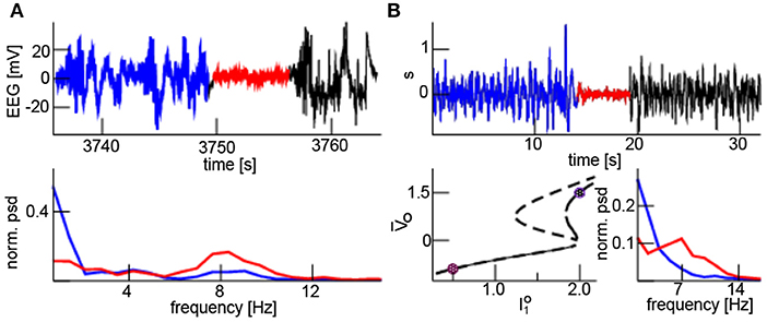
Figure 9. Neural burst suppression. (A) Experimental EEG with burst broad-band high-amplitude activity (blue and black) and the low-amplitude narrow band suppression (red) phase (top panel); the power spectral density of the burst (blue) and suppression (red) phase (bottom panel). (B, top) simulated EEG $s(t)={F}(\bar{V}(t))$ where ${F}$ represents a band pass filter (upper panel); high input has I₀ = 2.0, A = 0.04, D₁ = 1.2 for t ∈ [0s; 12.8s] and t ∈ [19.2s; 32.0s], low input I₀ = 0.5, A = 0.0, D₁ = 0.3 for t ∈ [12.8s; 19.2s]. (B, bottom) The dashed and solid line represents the equilibria for low (D₁ = 0.3) and high (D₁ = 1.2) additive noise levels, respectively; circles mark the high and low input with corresponding equilibrium (left). The normalized power spectral density of the burst (blue) and suppression (red) phase shows broad-band and phase-coherent states, respectively (right). In the model simulations, other parameters are taken from Figure 4 and time is re-scaled by t → 0.04t.

4. Discussion

In the present work, we have shown that both additive iid noise and non-iid noise, either through the form of fluctuations or heterogeneity, shape the dynamics of our two population model. This occurs because of an effective transformation of the non-linear interaction function: from a step function for vanishing noise over a symmetric sigmoid for non-vanishing homogeneous noise to a double-sigmoid function for heterogeneous noise. We present a fully analytical description of this system behavior in the context of oscillatory activity, and demonstrate that the system exhibits coherence resonance-like behavior. This enabled us to connect the dynamics to experimental observations, specifically the occurrence of burst suppression in human electroencephalographic data during general anesthesia.

The stochastic analysis implies several major assumptions:

• Homogeneity in Equation (2),

• Independent and identically distributed stationary stochastic processes in each noise class ${{G}}_m$ in Equation (4) reflecting ergodicity in each noise class and

• Statistical independence of connectivity matrix elements and stochastic process in Equation (12).

These assumptions are major conditions for the mean-field approach considered in the present work and they rule out the application to other network models, such as sparsely connected networks.

The network model in the present work is deliberately simple in order to allow the identification of major elements of the novel stochastic analysis. The model assumption of excitation-inhibition interaction is motivated by the well-known fact, that such interactions allows oscillatory activity. For instance, the balance between excitation and inhibition is an important mechanism in oscillatory biological neural networks [30, 38, 39]. Typical cortical neural networks have four times more excitatory than inhibitory synapses. Conversely, the networks ${V}$ and ${W}$ have identical number of nodes. This number relation has been chosen for simplicity reasons since the major stochastic effect is independent of the node number. Moreover, balanced networks exhibit an identical level of excitation and inhibition, i.e., γ = 1 in Figures 2, 3. Conversely, parameters in the model, e.g., the constant external inputs and the noise level, have been chosen for simplicity in order to demonstrate and visualize well the stochastic transitions by iid and non-iid noise. These parameters imply γ < 1, i.e., smaller excitation than inhibition, whereas different external input may allow γ > 1 as well. Since a corresponding detailed parameter study would well exceed the major aim of the present work, we refer the reader to forthcoming work.

We point out that the gained results are expected in other network topologies as well, just retaining the homogeneity condition (2) and the statistical independence of connectivity and external noise (12). For instance, previous studies have proposed different network topologies to model the brain that fulfill these conditions [3, 49]. However, these conditions may not hold for other models, such as sparsely connected networks [23], clustered networks [38], or scale-free networks [50]. Moreover, we point out that the present model describes the microscopic dynamics of two single interacting populations similar to the Wilson-Cowan model [25] and the homogeneity assumption is reasonable. This means the resulting model describes the dynamics on a larger, mesoscopic, scale. Conversely, previous studies using connectivity data from the brain connectome [3, 26] target the global brain dynamics, where each node may obey a Wilson-Cowan population dynamics. In such studies, the underlying connectivity matrices are macroscopic and non-homogeneous.

Our work adds to previous work [13, 36, 49] highlighting the importance of noise in shaping mesoscopic-scale brain activity. The considered network model may represent a single mesoscopic node in a larger macroscopic network model of the brain. In such macroscopic networks, the noise considered in our model may originate from other mesoscopic populations. Since such distant populations may oscillate and fluctuate randomly, future work will investigate a superposition of oscillatory and noisy external input.

Data Availability Statement

The datasets generated for this study are available on request to the corresponding author.

Ethics Statement

This study was approved by the Canton of Bern Ethics Committee. The patients/participants provided their written informed consent to participate in this study.

Author Contributions

AH and JL conceived the study and performed all calculations. DH and HK have provided the data and expertise in anesthesia and EEG. All authors have written the manuscript.

Conflict of Interest

The authors declare that the research was conducted in the absence of any commercial or financial relationships that could be construed as a potential conflict of interest.

Supplementary Material

The Supplementary Material for this article can be found online at: https://www.frontiersin.org/articles/10.3389/fams.2019.00069/full#supplementary-material

References

1. Sagues F, Sancho J, Garcia-Ojalvo J. Spatiotemporal order out of noise. Rev Mod Phys. (2007) 79:829–82. doi: 10.1103/RevModPhys.79.829

CrossRef Full Text | Google Scholar

2. Bratsun D, Volfson D, Tsimring L, Hasty J. Delay-induced stochastic oscillations in gene regulation. Proc Natl Acad Sci USA. (2013) 102:14593–8. doi: 10.1073/pnas.0503858102

PubMed Abstract | CrossRef Full Text | Google Scholar

3. Deco G, Jirsa V, McIntosh A, Sporns O, Kötter R. Key role of coupling, delay, and noise in resting brain fluctuations. Proc Natl Acad Sci USA. (2009) 106:10302–7. doi: 10.1073/pnas.0901831106

PubMed Abstract | CrossRef Full Text | Google Scholar

4. Doiron B, Lindner B, Longtin A, LMaler, Bastian J. Oscillatory activity in electrosensory neurons increases with the spatial correlation of the stochastic input stimulus. Phys Rev Lett. (2004) 93:048101. doi: 10.1103/PhysRevLett.93.048101

PubMed Abstract | CrossRef Full Text | Google Scholar

5. Wiesenfeld K, Moss F. Stochastic resonance and the benefits of noise: from ice ages to crayfish and squids. Nature. (1995) 373:33–6. doi: 10.1038/373033a0

PubMed Abstract | CrossRef Full Text | Google Scholar

6. Faisal A, Selen L, Wolpert D. Noise in the nervous system. Nat Rev Neurosci. (2008) 9:292–303. doi: 10.1038/nrn2258

PubMed Abstract | CrossRef Full Text | Google Scholar

7. Garcia-Ojalvo J, Sancho J. Noise in Spatially Extended Systems. New York, NY: Springer (1999).

PubMed Abstract | Google Scholar

8. Nicolis G, Prigogine I. Self-Organization in Non-Equilibrium Systems: From Dissipative Structures to Order Through Fluctuations. New York, NY: J. Wiley and Sons (1977).

Google Scholar

9. Pradas M, Tseluiko D, Kalliadasis S, Papageorgiou D, Pavliotis G. Noise induced state transitions, intermittency and universality in the noisy Kuramoto-Sivashinsky equation. Phys Rev Lett. (2011) 106:060602. doi: 10.1103/PhysRevLett.106.060602

CrossRef Full Text | Google Scholar

10. Bianchi L, Bloemker D, Yang M. Additive noise destroys the random attractor close to bifurcations. Nonlinearity. (2016) 29:3934. doi: 10.1088/0951-7715/29/12/3934

CrossRef Full Text | Google Scholar

11. Hutt A, Longtin A, Schimansky-Geier L. Additive noise-induced turing transitions in spatial systems with application to neural fields and the Swift-Hohenberg equation. Phys D. (2008) 237:755–73. doi: 10.1016/j.physd.2007.10.013

CrossRef Full Text | Google Scholar

12. Lefebvre J, Hutt A. Additive noise quenches delay-induced oscillations. Europhys Lett. (2013) 102:60003. doi: 10.1209/0295-5075/102/60003

CrossRef Full Text | Google Scholar

13. Lefebvre J, Hutt A, Knebel J, Whittingstall K, Murray M. Stimulus statistics shape oscillations in nonlinear recurrent neural networks. J Neurosci. (2015) 35:2895–903. doi: 10.1523/JNEUROSCI.3609-14.2015

PubMed Abstract | CrossRef Full Text | Google Scholar

14. Hutt A, Mierau A, Lefebvre J. Dynamic control of synchronous activity in networks of spiking neurons. PLoS ONE. (2016) 11:e0161488. doi: 10.1371/journal.pone.0161488

PubMed Abstract | CrossRef Full Text | Google Scholar

15. Lee KE, Lopes MA, Mendes FFF, Goltsev AV. Critical phenomena and noise-induced phase transitions in neuronal networks. Phys Rev E (2014) 89:012701. doi: 10.1103/PhysRevE.89.012701

PubMed Abstract | CrossRef Full Text | Google Scholar

16. Brunel N. Dynamics of networks of randomly connected excitatory and inhibitory spiking neurons. J Physiol. (2000) 94:445–63. doi: 10.1016/S0928-4257(00)01084-6

PubMed Abstract | CrossRef Full Text | Google Scholar

17. Haken H. Synergetics. Berlin: Springer (2004).

Google Scholar

18. Kelso J. Dynamic Patterns: The Self-Organization of Brain and Behavior. Cambridge: MIT Press (1995).

Google Scholar

19. Deghani N, Peyrache A, Telenczuk B, Le Van Quyen MEH, Cash S, Hatsopoulos N, et al. Dynamic balance of excitation and inhibition in human and monkey neocortex. Sci Rep. (2016) 6:23176. doi: 10.1038/srep23176

CrossRef Full Text | Google Scholar

20. Mahler H, Cordes E. Biological Chemistry. New York, NY: Harper and Row (1966).

Google Scholar

21. Ball P. The Self-made Tapestry–Pattern Formation in Nature. Oxford: Oxford University Press (1999).

Google Scholar

22. Niedermayer E. The burst-suppression electroencephalogram. Am J Electroneurodiagn Technol. (2009) 49:333–41. doi: 10.1080/1086508X.2009.11079736

CrossRef Full Text | Google Scholar

23. Amari S. Characteristics of sparsely encoded associative memory. Neural Netw. (1989) 2:451–7. doi: 10.1016/0893-6080(89)90043-9

CrossRef Full Text | Google Scholar

24. Hopfield J, Tank D. Computing with neural circuits: a model. Science. (1986) 233:625–33. doi: 10.1126/science.3755256

PubMed Abstract | CrossRef Full Text | Google Scholar

25. Wilson H, Cowan J. Excitatory and inhibitory interactions in localized populations of model neurons. Biophys J. (1972) 12:1–24. doi: 10.1016/S0006-3495(72)86068-5

PubMed Abstract | CrossRef Full Text | Google Scholar

26. Daffertshofer A, Ton R, Pietras B, Kringelbach ML, Deco G. Scale-freeness or partial synchronization in neural phase oscillator networks: pick one or two? Neuroimage. (2018) 180:428–41. doi: 10.1016/j.neuroimage.2018.03.070

CrossRef Full Text | Google Scholar

27. Hellwig B. A quantitative analysis of the local connectivity between pyramidal neurons in layers 2/3 of the rat visual cortex. Biol Cybern. (2000) 82:111–21. doi: 10.1007/PL00007964

PubMed Abstract | CrossRef Full Text | Google Scholar

28. Erdös P, Rényi A. On random graphs. I. Publ Math. (1959) 6:209–97.

Google Scholar

29. Risken H. The Fokker-Planck Equation|Methods of Solution and Applications. Berlin: Springer (1989).

Google Scholar

30. Hutt A. The anaesthetic propofol shifts the frequency of maximum spectral power in EEG during general anaesthesia: analytical insights from a linear model. Front Comp Neurosci. (2013) 7:2. doi: 10.3389/fncom.2013.00002

CrossRef Full Text | Google Scholar

31. Lachaux JP, Lutz A, Rudrauf D, Cosmelli D, Le Van Quyen M, Martinerie J, et al. Estimating the time course of coherence between single-trial signals: an introduction to wavelet coherence. Neurophysiol Clin. (2002) 32:157–74. doi: 10.1016/S0987-7053(02)00301-5

PubMed Abstract | CrossRef Full Text | Google Scholar

32. Boashash B. Estimating and interpreting the instantaneous frequency of a signal–part 1: fundamentals. Proc IEEE. (1992) 80:520–38. doi: 10.1109/5.135376

CrossRef Full Text | Google Scholar

33. Le Van Quyen M, Foucher J, Lachaux J, Rodriguez E, Lutz A, Martinerie J, et al. Comparison of hilbert transform and wavelet methods for the analysis of neuronal synchrony. J Neurosci Methods. (2001) 111:83–98. doi: 10.1016/S0165-0270(01)00372-7

PubMed Abstract | CrossRef Full Text | Google Scholar

34. Rosenblum M, Pikovsky A, Schafer C, Tass P, Kurths J. Phase synchronization: from theory to data analysis. Handb Biol Phys. (2000) 4:279–321. doi: 10.1016/S1383-8121(01)80012-9

CrossRef Full Text | Google Scholar

35. Hutt A, Munk M. Mutual phase synchronization in single trial data. Chaos Complex Lett. (2006) 2:6.

Google Scholar

36. Hutt A, Lefebvre J, Hight D, Sleigh J. Suppression of underlying neuronal fluctuations mediates EEG slowing during general anaesthesia. Neuroimage. (2018) 179:414–28. doi: 10.1016/j.neuroimage.2018.06.043

PubMed Abstract | CrossRef Full Text | Google Scholar

37. Herrmann CS, Murray MM, Ionta S, Hutt A, Lefebvre J. Shaping intrinsic neural oscillations with periodic stimulation. J Neurosci. (2016) 36:5328–39. doi: 10.1523/JNEUROSCI.0236-16.2016

PubMed Abstract | CrossRef Full Text | Google Scholar

38. Litwin-Kumar A, Doiron B. Slow dynamics and high variability in balanced cortical networks with clustered connections. Nat Neurosci. (2012) 15:1498. doi: 10.1038/nn.3220

PubMed Abstract | CrossRef Full Text | Google Scholar

39. Deneve S, Machens CK. Efficient codes and balanced networks. Nat Neurosci. (2006) 19:375. doi: 10.1038/nn.4243

PubMed Abstract | CrossRef Full Text | Google Scholar

40. Murray J. Mathematical Biology. Berlin: Springer (1989).

PubMed Abstract | Google Scholar

41. Klöden PE, Platen E. Numerical Solution of Stochastic Differential Equations. Heidelberg: Springer-Verlag (1992).

Google Scholar

42. Bloemker D. Amplitude equations for locally cubic non-autonomous nonlinearities. SIAM J Appl Dyn Syst. (2003) 2:464–86. doi: 10.1137/S1111111103421355

CrossRef Full Text | Google Scholar

43. Pikovsky A, Kurths J. Coherence resonance in a noise-driven excitable system. Phys Rev Lett. (1997) 78:775–8. doi: 10.1103/PhysRevLett.78.775

CrossRef Full Text | Google Scholar

44. Beato V, Sendina-Nadal I, Gerdes I, Engel H. Coherence resonance in a chemical excitable system driven by coloured noise. Philos Trans A Math Phys Eng Sci. (2008) 366:381–95. doi: 10.1098/rsta.2007.2096

PubMed Abstract | CrossRef Full Text | Google Scholar

45. Yu Y, Liu F, Wang W. Synchronized rhythmic oscillation in a noisy neural network. J Phys Soc. (2003) 72:3291–6. doi: 10.1143/JPSJ.72.3291

CrossRef Full Text | Google Scholar

46. Steriade M. Arousal–revisiting the reticular activating system. Science. (1996) 272:225. doi: 10.1126/science.272.5259.225

PubMed Abstract | CrossRef Full Text | Google Scholar

47. Carstens E, Antognini J. Anesthetic effects on the thalamus, reticular formation and related systems. Thal Rel Syst. (2005) 3:1–7. doi: 10.1017/S1472928805000014

CrossRef Full Text | Google Scholar

48. Glackin C, Maguire L, McDaid L, Wade J. Lateral inhibitory networks: synchrony edge enhancement and noise reduction. In: Proceedings on IEEE International Joint Conference on Neural Networks. San Jose, CA (2011). p. 1003–9.

Google Scholar

49. Lefebvre J, Hutt A, Frohlich F. Stochastic resonance mediates the state-dependent effect of periodic stimulation on cortical alpha oscillations. eLife. (2017) 6:e32054. doi: 10.7554/eLife.32054

PubMed Abstract | CrossRef Full Text | Google Scholar

50. Di Santo S, Villegas P, Burioni R, Munoz MA. Landau-Ginzburg theory of cortex dynamics: scale-free avalanches emerge at the edge of synchronization. Proc Natl Acad Sci USA. (2018) 115:E1356–65. doi: 10.1073/pnas.1712989115

PubMed Abstract | CrossRef Full Text | Google Scholar