A Reaction–Diffusion–Advection Model for the Establishment and Maintenance of Transport-Mediated Polarity and Symmetry Breaking

1 Introduction

The development and maintenance of cell polarity is essential for many biological processes like cell growth, cell morphogenesis, cell migration, cell differentiation, proliferation, and signal transmission. Also known as symmetry breaking, it describes the process by which cells generate an internal, functional, structural, and molecular axis. This asymmetric arrangement often arises due to intrinsic or extrinsic cues which are amplified by transport processes or pathways of diffusing and interacting molecules. The budding yeast (Saccharomyces cerevisiae) is an exemplary model system to study the underlying mechanisms of cell polarization. Whereas in these cells, the small family GTPase Cdc42 is a key regulator of cell polarity, GTPases in general are exemplary for a complex system with symmetry breaking in many eukaryotic cells [8, 13, 28].

GTPase molecules are able to change between three forms: an active (GTP-bound) membrane-bound state, an inactive (GDP-bound) membrane-bound state, and an inactive (GDI-bound) cytosolic state. The regulation of this cycle is controlled by certain exchange factors, GEFs (GTPase-activating proteins), GAPs (guanine nucleotide exchange factors), and GDIs (GTPase dissociation inhibitors), leading to shuttling between the cytosol and the plasma membrane [8, 16, 29]. Thus, the GTPase cycle is characterized by a coupled bulk (cytosol) and surface (plasma membrane) reaction–diffusion system.

Since coupled bulk-surface reaction–diffusion systems naturally arise in many biological processes, a huge number of studies concerning such systems, like, for example, Refs. 18, 21, and 23, has recently been published. All these models were always based on reaction–diffusion equations posed on the bulk and surface coupled by Robin-type boundary conditions which generate symmetry breaking by Turing-type instabilities. But many cells exhibit a transport machinery characterized by actin filaments or microtubules (see, e.g., Refs. 9, 19, 24, and 31), which further influence spatial patterns. For example, the budding yeast generates polarity by the coupling of reaction–diffusion to transport systems. Actin cables which are aligned along the plasma membrane transport vesicles containing key proteins required for cell polarization from the interior of the cell to the polarized site (exocytosis) [32]. Simultaneously, molecules are internalized from the plasma membrane to the interior of the cell (endocytosis). To simulate vesicular mediated transport, stochastic equations were commonly used, see e.g. [14, 17]. It is observed that transport-mediated recycling of molecules plays a key role in polarity establishment and maintenance as well [33]. For that reason, here, we consider a coupled bulk-surface reaction–diffusion–advection system to investigate the contribution of transport to cell polarity. Following the approach proposed in Ref. 23, we perform a linear stability analysis and derive conditions for a transport-mediated instability, which are confirmed numerically.

Contribution of This Paper

Our main contribution is a continuous model for vesicle transport based on active transport, together with an analysis of its contribution to symmetry breaking. Previous models of actin-mediated polarization were solely based on stochastic simulations [9]. Our continuous PDE model allows for a better characterization of the conditions for polarization.

In Section 2, we introduce the model in its nondimensional form. For details on the model reduction and nondimensionalization, we refer to the Supplementary Material. In Section 3, we analyze in detail under which conditions the model can induce pattern formation and complement these results by numerical experiments in Section 4. The stability results confirm that actin-mediated Cdc42 recruitment can increase the robustness of the system. And, we show the ability of the system to polarize via two independent pathways, as it was observed in experiments for budding yeast cells [27, 33].

We further investigate numerically the interplay of active transport and geometrical features like organelles, where our experiments indicate that the presence an actin-mediated pathway accelerates polarization and can even induce different patterns.

We conclude with a discussion on the biological implications of our numerical findings.

2 Model Description

We consider a generic reaction–diffusion–transport system that is based on a complex model for cell polarization proposed in [6]. This model was motivated by the influence of vesicle transport along actin cables on the cell polarization, as described in Refs. 9 and 33 (see Supplementary Material for model reduction and nondimensionalization). This system differentiates among one active membrane-bound, one inactive membrane-bound, and a cytosolic state. This model includes the distribution of actin cables on the membrane as an additional component. Its dynamics are described by an inhomogeneous diffusion proportional to the membrane-bound component modeling the described transport-mediated feedback loop.

In the following, we consider a stationary bulk domain $\text{Ω}$ and its compact hypersurface $\text{Γ}:=\partial \text{Ω}$. We denote by $\overrightarrow{n}$ the outer normal on the smooth, closed surface $\text{Γ}$, by ${\nabla }_{\text{Γ}}$ the tangential gradient on $\text{Γ}$ and the Laplace–Beltrami operator ${\text{Δ}}_{\text{Γ}}$.

Let $u,v:\text{Γ}\times I\to \mathrm{ℝ}$ be smooth functions denoting the chemical concentrations or species that react and diffuse on $\text{Γ}$ in a fixed time interval $I:=[0,T]\subset \mathrm{ℝ}$. For substances that diffuse or move by advection in the volume $\text{Ω}\subset {\mathrm{ℝ}}^n$, we consider smooth functions $U,V:\text{Ω}\times I\to \mathrm{ℝ}$. To proceed, we denote by $w:\text{Γ}\times I\to \mathrm{ℝ}$, a smooth function representing a transport control factor, in our case, the density of actin cable ends on the surface $\text{Γ}$. Furthermore, $c\left(u\right)>0$ describes a capacity function controlling w and hence impacts actin cable assembly. This model follows the observation that actin is essential for cell polarization [1], and vesicle transport (in yeast cells) happens along actin cables. We further include the fact that actin has a reduced dissociation rate, where Cdc42 concentration is high [33], which leads to a u-dependent actin density in the membrane. We model this by an inhomogeneous diffusion and the nonlinear capacity function $c\left(u\right)$. Where c is large, the likelihood for actin to bind is high, whereas a small c increases the probability that the actin cable moves away. Further details can be found in the Supplementary Material.

This leads to the following nondimensional coupled reaction–diffusion–advection system

${\partial }_{t}u={\text{Δ}}_{\text{Γ}}u+\gamma \left(f\left(u,v\right)+h\left(u,w,U\right)\right)\text{on Γ}\times I,(\mathrm{1a})$

${\partial }_{t}v=d_v{\text{Δ}}_{\text{Γ}}v+\gamma \left(-f\left(u,v\right)+g\left(u,v,V\right)\right)\text{on Γ}\times I,(\mathrm{1b})$

${\partial }_{t}w=d_w{\text{Δ}}_{\text{Γ}}\left(w\cdot c{\left(u\right)}^{-1}\right)\text{on Γ}\times I,(\mathrm{1c})$

${\partial }_{t}U=D_u\text{Δ}U-\nabla \cdot \left(\overrightarrow{v}U\right)\text{in Ω}\times I,(\mathrm{1d})$

${\partial }_{t}V=D_v\text{Δ}V\text{in Ω}\times I,(1e)$

with coupling conditions

$-D_u\nabla U\cdot \overrightarrow{n}=\gamma h\left(u,w,U\right)\text{on Γ}\times I,(\mathrm{1f})$

$-D_v\nabla V\cdot \overrightarrow{n}=\gamma g\left(u,v,V\right)\text{on Γ}\times I,(\mathrm{1g})$

and initial conditions at time $t=0$

$\begin{array}{l}U(\cdot ,0)=U_0>0, V(\cdot ,0)=V_0>0\text{in }\Omega \\ \text{and}u(\cdot ,0)=u_0>0, v(\cdot ,0)=v_0>0, w(\cdot ,0)=w_0>0\text{on }\Gamma .\end{array}(2)$

Here, the nonlinear functions f and g, respectively, represent activation and inactivation of the species, h describes adsorption and desorption of molecules, and $\overrightarrow{v}$ is the divergence-free bulk velocity field. The parameters $D_U$ and $D_V$ denote the nondimensional bulk diffusion coefficients and $d_v,d_w>0$ the surface diffusion coefficients, which are assumed to be constant. The nondimensional parameter $\gamma >0$ relates to the spatial scale of the cell.

REMARK 2.1 (mass conservation). Note that this formulation implies conservation of mass. This means that with dσ denoting the integration with respect to the surface area measure and M the total mass, the system satisfies the condition

$\frac{d}{dt}M=\frac{d}{dt}\left[\underset{\text{Ω}}{{\displaystyle \int }}\left[U\left(x,t\right)+V\left(x,t\right)\right]dx+\underset{\text{Γ}}{{\displaystyle \int }}\left[u\left(x,t\right)+v\left(x,t\right)+w\left(x,t\right)\right]d\sigma \left(x\right)\right]=0.$

REMARK 2.2 (velocity field). As vesicles only release their content when being integrated into the membrane, the velocity field $\overrightarrow{v}$ is conservative, that is, divergence free.

The outflow rate on the membrane depends (potentially nonlinear) on the concentration w of actin cable ends on the membrane. Given an outflow function $j\left(w\right)$, we construct a divergence-free velocity field $\overrightarrow{v}=\nabla \varphi$ as the gradient of a scalar function ϕ. This potential flow from the internal to the external membrane is caused by constructing a divergence-free velocity field and is computed by solving.

$0=\text{Δ}\varphi -\alpha \varphi in \text{Ω}\times I,$

$\nabla \varphi \cdot \overrightarrow{n}=j\left(w\right)on \partial \text{Ω}=\text{Γ},$

where α describes a potential flow control rate, which limits the transport capacity.

3 Linear Stability Analysis

Here, we present a stability analysis of the generic system which mainly follows the analysis shown in Ref. 23, to determine conditions required for pattern formation. We restrict ourselves to the spherical case, that is, $\text{Ω}:=B_1\left(0\right)$, $\text{Γ}:=\partial B=S^2$.

We assume that the internal pool is sufficiently large and that $D_u\gg 1$. This ensures a well-mixed internal pool, similar to the assumptions in Ref. 23, so that the feedback loop between the component u (active form) and w (actin) is dominating. This simplification has clear limits; in particular, it cannot handle any transport-limited cases. The validity of this assumption will be backed by the numerical simulations in Section 4.2, comparing the full model with the simplified coupling used in the following analysis.

As the rate of transport indirectly depends on the amount of w on $\text{Γ}$, the actin concentration on the membrane is now only governed by an inhomogeneous diffusion controlled by the capacity function $c\left(u\right)$, and we can substitute $\tilde{w}:=w\cdot c{\left(u\right)}^{-1}$ in Eq. 1c.

The system Eq. 1 then reads

${\partial }_{t}u={\text{Δ}}_{\text{Γ}}u+\gamma \left(f\left(u,v\right)+h\left(u,c\left(u\right)\cdot \tilde{w},U\right)\right)\text{on Γ}\times I,(\mathrm{3a})$

${\partial }_{t}v=d_v{\text{Δ}}_{\text{Γ}}v+\gamma \left(-f\left(u,v\right)+g\left(u,v,V\right)\right)\text{on Γ}\times I,(\mathrm{3b})$

$c\left(u\right)\cdot {\partial }_t\tilde{w}=d_w{\text{Δ}}_{\gamma }\tilde{w}\text{on Γ}\times I,(\mathrm{3c})$

${\partial }_{t}U=D_u\text{Δ}U\text{in Ω}\times I,(\mathrm{3d})$

${\partial }_{t}V=D_v\text{Δ}V\text{in Ω}\times I,(3e)$

with Robin-type coupling conditions.

$-D_u\nabla U\cdot \overrightarrow{n}=\gamma h\left(u,c\left(u\right)\cdot \tilde{w},U\right)\text{on Γ}\times I,(\mathrm{3f})$

$-D_v\nabla V\cdot \overrightarrow{n}=\gamma g\left(u,v,V\right)\text{on Γ}\times I,(\mathrm{3g})$

and the initial conditions (2). In the following, we will denote by $x:={\left(u,v,w,U,V\right)}^T$ the vector of concentrations and by $x_{\text{*}}:=\left(u_{\text{*}},v_{\text{*}},w_{\text{*}},U_{\text{*}},V_{\text{*}}\right)\in {\mathrm{ℝ}}_{+}^5$ the spatially homogeneous steady state, such that

$f\left(u_{\text{*}},v_{\text{*}}\right)=0,g\left(u_{\text{*}},v_{\text{*}},V_{\text{*}}\right)=0,\text{and}h\left(u_{\text{*}},w_{\text{*}},V_{\text{*}}\right)=0.$

Following the approach of Ref. 23, we analyze the stability of system Eq. 1 at its stationary states. Focusing on the GTPase cycle, we can interpret f as an activation rate and g as the flux describing membrane attachment and detachment of the GTPase. The function h describes the flux induced by exocytosis and endocytosis. This interpretation corresponds to the following conditions on $f,g,$ and h

${\partial }_{v}f\ge 0,{\partial }_{v}g\le 0,{\partial }_{v}g\le {\partial }_{u}g,\text{and}{\partial }_{U}h\ge 0.$

For brevity, we introduce the notation

$f_u:={\partial }_{u}f(u_{\text{*}},v_{\text{*}}),f_v:={\partial }_{v}f(u_{\text{*}},v_{\text{*}}),$

$g_u:={\partial }_{u}g(u_{\text{*}},v_{\text{*}},V_{\text{*}}),g_v:={\partial }_{v}g(u_{\text{*}},v_{\text{*}},V_{\text{*}}),g_V:={\partial }_{V}g(u_{\text{*}},v_{\text{*}},V_{\text{*}}),$

$h_u:={\partial }_{u}h(u_{\text{*}},w_{\text{*}},U_{\text{*}}),h_w:={\partial }_{w}h(u_{\text{*}},w_{\text{*}},U_{\text{*}}),h_U:={\partial }_{U}h(u_{\text{*}},w_{\text{*}},U_{\text{*}}),$

assuming that at $s_{\text{*}}=\left(u_{\text{*}},v_{\text{*}},w_{\text{*}},U_{\text{*}},V_{\text{*}}\right)$, the functions satisfy the strict inequalities

$f_v>0,g_v<0,g_V>0,\text{and }{h}_U>0.(4)$

As in Ref. 23, to determine stability conditions for the system Eq. 3, we use an expansion in spherical harmonics:

$\left(\begin{array}{c}u\\ v\\ \tilde{w}\\ U\\ V\end{array}\right)\left(p,t\right)={\displaystyle \sum }_{l\in {\mathrm{\mathbb{N}}}_0,m\in \mathrm{\mathbb{Z}},\left|m\right|\le l}\left(\begin{array}{c}{u}_{lm}\left(t\right)\\ v_{lm}\left(t\right)\\ {\tilde{w}}_{lm}\left(t\right)\\ U_{lm}\left(t\right){\psi }_{lm}\left(r\right)\\ V_{lm}\left(t\right){\chi }_{lm}\left(r\right)\end{array}\right){\phi }_{lm}\left(p\right),$

with scalar functions ${\psi }_{lm},{\chi }_{lm}:\left[\mathrm{0,1}\right]\to \mathrm{ℝ}$, and the orthonormal basis ${\left\{{\phi }_{lm}\right\}}_{l\in {\mathrm{\mathbb{N}}}_0,m\in \mathrm{\mathbb{Z}},\left|m\right|\le l}$ of $L^2\left(\text{Γ}\right)$. Then, the Laplace operator can be represented as

$-{\text{Δ}}_{\text{Γ}}{\phi }_{lm}=l\left(l+1\right){\phi }_{lm}\text{on}\text{Γ}.$

As a result, the $L^2\left(\text{Γ}\right)$ scalar product with ${\phi }_{lm}$ leads to the linearized system

$\begin{array}{c}{u}_{lm}^{\text{′}}=-\left(l+1\right)u_{lm}+\gamma \left(\left(f_u+h_u+c_u\widetilde{w_{\text{*}}}{h}_w\right)u_{lm}+f_v{v}_{lm}\right)\\ +\gamma \left(c\left(u_{\text{*}}\right)h_w{\tilde{w}}_{lm}+h_U{\psi }_{lm}\left(1\right)U_{lm}\right),\end{array}(\mathrm{5a})$

$\begin{array}{c}{v}_{lm}^{\text{′}}=-d_v(l+1)v_{lm}+\gamma (-f_u+g_u)u_{lm}+(-f_v+g_v)v_{lm})\\ +\gamma g_V{\psi }_{lm}\left(1\right)V_{lm},\end{array}(\mathrm{5b})$

$c\left(u\right){\tilde{w}}_{lm}^{\text{′}}=d_{w}l\left(l+1\right){\tilde{w}}_{lm},(\mathrm{5c})$

$U_{lm}^{\text{′}}\left(t\right)\psi \left(r\right)=D_u{U}_{lm}\left(t\right)\left({\psi }_{lm}^{″}\left(r\right)+\frac{2}{r}{\psi }_{lm}^{\text{′}}\left(r\right)-\frac{1}{r^2}l\left(l+1\right){\psi }_{lm}\left(r\right)\right),(\mathrm{5d})$

$V_{lm}^{\prime }\left(t\right)\chi \left(r\right)=D_v{V}_{lm}\left(t\right)\left({\chi }_{lm}^{″}\left(r\right)+\frac{2}{r}{\chi }_{lm}^{\prime }\left(r\right)-\frac{1}{r^2}l\left(l+1\right){\chi }_{lm}\left(r\right)\right),(5e)$

$-D_v{U}_{lm}{\psi }_{lm}\left(1\right)=\gamma \left(\left(h_u+c_u\widetilde{w_{\text{*}}}{h}_w\right)u_{lm}+c\left(u_{\text{*}}\right)h_w{\tilde{w}}_{lm}+h_U{\psi }_{lm}\left(1\right)U_{lm}\right),.(\mathrm{5f})$

$-D_v{V}_{lm}{\chi }_{lm}\left(1\right)=\gamma \left(g_u{u}_{lm}+g_v{v}_{lm}+g_V{\chi }_{lm}\left(1\right)V_{lm}\right),(\mathrm{5g})$

where the last two equations correspond to the coupling conditions. We use the following ansatz:

$U_{lm}\left(t\right)={\overline{B}}_{lm}{e}^{{\lambda }_{lm}t},{\overline{B}}_{lm}\in \mathrm{ℝ},{\lambda }_{lm}\in \mathrm{ℝ},$

$V_{lm}\left(t\right)={\overline{B}}_{lm}{e}^{{\mu }_{lm}t},{\overline{B}}_{lm}\in \mathrm{ℝ},{\mu }_{lm}\in \mathrm{ℝ},$

which also guarantees that either $U_{lm},V_{lm}\ne 0$ in the whole domain or are identical to zero.

We first consider the case $U_{lm},V_{lm}\ne 0$. Then, using $U_{lm}^{\text{′}}={\lambda }_{lm}{U}_{lm}$ and $V_{lm}^{\text{′}}={\mu }_{lm}{V}_{lm}$, we obtain from Eqs. 5d and 5e

$0=r^2{\psi }_{lm}^{\text{′}\text{′}}\left(r\right)+2r{\chi }_{lm}^{\text{′}}\left(r\right)-\left(l\left(l+1\right)+\frac{{\lambda }_{lm}}{D_u}{r}^2\right){\psi }_{lm}\left(r\right),(\mathrm{6a})$

$0=r^2{\chi }_{lm}^{\text{′}\text{′}}\left(r\right)+2r{\chi }_{lm}^{\text{′}}\left(r\right)-\left(l\left(l+1\right)+\frac{{\mu }_{lm}}{D_v}{r}^2\right){\chi }_{lm}\left(r\right).(\mathrm{6b})$

In the case ${\lambda }_{lm},{\mu }_{lm}=0$, it is easy to recalculate that we have

${\psi }_{lm}\left(r\right)={\alpha }_{lm}{r}^l,{\chi }_{lm}\left(r\right)={\beta }_{lm}{r}^l,$

with ${\alpha }_{lm},{\beta }_{lm}\in \mathrm{ℝ}$. By contrast, for ${\lambda }_{lm},{\mu }_{lm}>0$, Eqs. 6a and 6b are modified versions of Bessel differential equations whose solutions are defined by Bessel functions of first kind. Hence, using the respective modified Bessel function $J_{l+\frac{1}{2}}$, we derive

$\psi \left(r\right)={\alpha }_{lm}{\xi }_l\left(\sqrt{\frac{{\lambda }_{lm}}{D_u}}r\right),\alpha \in \mathrm{ℝ},\chi \left(r\right)={\beta }_{lm}{\xi }_l\left(\sqrt{\frac{{\mu }_{lm}}{D_v}}r\right),\beta \in \mathrm{ℝ},$

with ${\xi }_l=\sqrt{\frac{\pi }{2r}}{\text{J}}_{\text{l}+\frac{1}{2}}\left(r\right)$. With this, we finally deduce the ODE system

$u_{lm}^{\text{′}}=\left(-l\left(l+1\right)+\gamma f_u\right)u_{lm}+\gamma f_v{v}_{lm}-D_u{\psi }_{lm}^{\text{′}}\left(1\right)U_{lm},(\mathrm{7a})$

$v_{lm}^{\text{′}}=-\gamma f_u{u}_{lm}-\left(d_{v}l\left(l+1\right)+\gamma f_v\right)v_{lm}-D_v{\chi }_{lm}^{\text{′}}\left(1\right)V_{lm},(\mathrm{7b})$

$c\left(u\right){\tilde{w}}_{lm}^{\text{′}}=-d_{w}l\left(l+1\right){\tilde{w}}_{lm},(\mathrm{7c})$

$U_{lm}^{\text{′}}={\lambda }_{lm}{U}_{lm},(\mathrm{7d})$

$V_{lm}^{\text{′}}={\mu }_{lm}{V}_{lm},(7e)$

coupled to two algebraic equations given by

$0=\gamma \left(\left(h_u+c_u\widetilde{w_{\text{*}}}{h}_w\right)u_{lm}+c\left(u_{\text{*}}\right)h_w{\tilde{w}}_{lm}\right)+\left(\gamma h_U{\psi }_{lm}\left(1\right)+D_u{\psi }_{lm}^{\text{′}}\left(1\right)\right)U_{lm},$

$0=\gamma \left(g_u{u}_{lm}+g_v{v}_{lm}\right)+\left(\gamma g_V{\chi }_{lm}\left(1\right)+D_v{\chi }_{lm}^{\text{′}}\left(1\right)\right)V_{lm}.$

We introduce the notation

$x{\text{'}}_{lm}:=\left(\begin{array}{c}{u}_{lm}^{\text{′}}\\ v_{lm}^{\text{′}}\\ c\left(u\right){\tilde{w}}_{lm}^{\text{′}}\\ U_{lm}^{\text{′}}\\ V_{lm}^{\text{′}}\end{array}\right),x_{lm}:=\left(\begin{array}{c}{u}_{lm}\\ v_{lm}\\ {\tilde{w}}_{lm}\\ U_{lm}\\ V_{lm}\end{array}\right),$

and the jacobian matrix is the system is given as

${\mathbf{J}}_F:=\left(\begin{array}{ccccc}-l\left(l+1\right)+\gamma f_u& \gamma f_v& 0& -D_u{\psi }_{lm}^{\text{′}}\left(1\right)& 0\\ -\gamma f_u& -d_{v}l\left(l+1\right)-\gamma f_v& 0& 0& -D_v{\chi }_{lm}^{\text{′}}\left(1\right)\\ 0& 0& -d_{w}l\left(l+1\right)& 0& 0\\ \gamma \left(h_u+c_u\widetilde{w_{\text{*}}}{h}_w\right)& 0& \gamma c\left(u_{\text{*}}\right)h_w& \xi & 0\\ \gamma g_u& \gamma g_v& 0& 0& \eta \end{array}\right),$

with

$\xi :=\gamma h_U{\psi }_{lm}\left(1\right)+D_u{\chi }_{lm}^{\text{′}}\left(1\right)+{\lambda }_{lm},$

$\eta :=\gamma g_V{\chi }_{lm}\left(1\right)+D_v{\chi }_{lm}^{\text{′}}\left(1\right)+{\mu }_{lm}.$

Writing

$x_{lm}^{\text{′}}={\mathbf{J}}_F{x}_{lm},$

the stability analysis reduces to an analysis of the eigenvalues of the matrix ${\mathbf{J}}_F$. To determine stability conditions, we compute eigenvalues λ of ${\mathbf{J}}_F$via the characteristic polynomial

$\begin{array}{c}{P}_l\left(\lambda \right)=p_{l,1}\left(\lambda \right)[\left(\gamma g_V{\chi }_{lm}\left(1\right)+D_v{\chi }_{lm}^{\text{′}}\left(1\right)+{\mu }_{lm}-\lambda \right)\cdot \left(\gamma h_U{\psi }_{lm}\left(1\right)+D_u{\psi }_{lm}^{\text{′}}\left(1\right)+{\lambda }_{lm}-\lambda \right)]\\ +p_{l,2}\left(\lambda \right)[\left(\gamma h_U{\psi }_{lm}\left(1\right)+D_u{\psi }_{lm}^{\text{′}}\left(1\right)+{\mu }_{lm}-\lambda \right)\cdot D_u{\psi }_{lm}^{\text{′}}\left(1\right)]\\ +p_{l,3}\left(\lambda \right)[\left(\gamma g_V{\chi }_{lm}\left(1\right)+D_v{\chi }_{lm}^{\text{′}}\left(1\right)+{\lambda }_{lm}-\lambda \right)\cdot {\chi }_{lm}^{\text{′}}\left(1\right)]\\ +p_{l,4}\left(\lambda \right)[D_u{\psi }_{lm}^{\text{′}}\left(1\right)\cdot D_v{\chi }_{lm}^{\text{′}}\left(1\right)],\end{array}(8)$

with

$\begin{array}{l}{p}_{l,1}\left(\lambda \right)={\lambda }^2+[\left(d_v+1\right)\left(l+1\right)l+\left(-f_u+f_v\right)\gamma ]\lambda +d_v{l}^2{\left(l+1\right)}^2\\ +\gamma \left(l\left(l+1\right)\right)\left(-d{f}_u+f_v\right),\\ p_{l,2}\left(\lambda \right)=[-l\left(l+1\right)+\gamma f_u-\lambda ]\gamma g_v-{\gamma }^2{f}_v{g}_u\\ p_{l,3}\left(\lambda \right)=[-d_{v}l\left(l+1\right)-\gamma f_v-\lambda ]\gamma \left(h_u+c_u{\tilde{w}}_{\text{*}}{h}_w\right)\\ p_{l,4}\left(\lambda \right)={\gamma }^2{g}_v\left(h_u+c_u{\tilde{w}}_{\text{*}}{h}_u\right).\end{array}$

The eigenvalues are now given by the zeros of polynomial (8). Hence, from Eqs. 7a–7e, as long as $U_{lm},V_{lm}\ne 0$, we acquire that an eigenvalue λ with $\text{Re}\left(\lambda \right)>0$ exists if and only if first $\lambda ={\lambda }_{lm}={\mu }_{lm}\in {\mathrm{ℝ}}_0^{+}$ and additionally with

${\kappa }_{D_u,l}\left(\lambda \right):=\frac{D_u{\psi }_{lm}^{\text{′}}\left(1\right)}{{\psi }_{lm}\left(1\right)}={D_u\left(\frac{r{\xi }_l^{\text{′}}\left(r\right)}{{\xi }_l\left(r\right)}\right)|}_{r=\sqrt{\frac{\lambda }{D_u}}},(\mathrm{9a})$

${\kappa }_{D_v,l}\left(\lambda \right):=\frac{D_v{\chi }_{lm}^{\text{′}}\left(1\right)}{{\chi }_{lm}\left(1\right)}={D_v\left(\frac{r{\xi }_l^{\text{′}}\left(r\right)}{{\xi }_l\left(r\right)}\right)|}_{r=\sqrt{\frac{\lambda }{D_v}}}.(\mathrm{9b})$

${\lambda }_{lm}$ fulfills the condition

$\begin{array}{c}{P}_l\left({\lambda }_{lm}\right):=\left(\gamma g_V+{\kappa }_{D_v,l}\left({\lambda }_{lm}\right)\right)\cdot \left(\gamma h_U+{\kappa }_{D_u,l}\left({\lambda }_{lm}\right)\right)\cdot p_{l,1}\left({\lambda }_{lm}\right)\\ +\left(\gamma h_U+{\kappa }_{D_u,l}\right)\cdot {\kappa }_{D_v,l}\cdot p_{l,2}\left({\lambda }_{lm}\right)\\ +\left(\gamma g_V+{\kappa }_{D_v,l}\right)\cdot {\kappa }_{D_u,l}\cdot p_{l,3}\left({\lambda }_{lm}\right)\\ +{\kappa }_{D_u,l}\cdot {\kappa }_{D_v,l}\cdot p_{l,4}\left({\lambda }_{lm}\right)\stackrel{!}{=}0.\end{array}$

Proposition 3.1. In $\left(u_{\text{*}},v_{\text{*}},w_{\text{*}},U_{\text{*}},V_{\text{*}}\right)$, the system (3) is stable against spatially homogeneous perturbations in the variables $u,v$, and w if the following condition is satisfied:

$\frac{1}{3}\left(f_u{g}_v{h}_U-f_v{g}_u{h}_U-g_V{h}_u{f}_u\right)+g_V{h}_U\left(f_v-f_u\right)>0,(10)$

in which case

$f_v-f_u>h_u>0$

holds.

If either U or $V=0$, we distinguish two cases and conclude that in

Case 1 ($U=0$),

$\frac{1}{3}\left(f_u{g}_v-f_v{g}_u\right)+g_V\left(f_v-f_u\right)>0\Rightarrow f_v>f_u,(11)$

Case 2 ($\text{V}=0$)

$h_U\left(f_v-f_u\right)-\frac{1}{3}{f}_v{h}_u>0\Rightarrow h_u<0,(12)$

holds.

Proof. We first consider the case $l=0$. Furthermore, we assume that $U_{00},V_{00}\ne 0$. Note that in this case, w is always constant and $w=w_0$. This also implies $h_w=0$. Then, the characteristic polynomial Eq. 8 reduces to

$\begin{array}{c}{P}_0\left(\lambda \right)=\left(\gamma g_V+{\kappa }_{D_v,l}\left(\lambda \right)\right)\cdot \left(\gamma h_U+{\kappa }_{D_u,l}\left(\lambda \right)\right)\cdot [{\lambda }^2+\left(-f_u+f_v\right)\gamma \lambda ]\\ +\left(\gamma h_U+{\kappa }_{D_u,l}\left(\lambda \right)\right)\cdot {\kappa }_{D_v,l}\left(\lambda \right)\cdot [{\gamma }^2{f}_u{g}_v-\lambda \gamma g_v-{\gamma }^2{f}_v{g}_u]\\ +\left(\gamma g_V+{\kappa }_{D_v,l}\left(\lambda \right)\right)\cdot {\kappa }_{D_u,l}\left(\lambda \right)\cdot [-{\gamma }^2{f}_v{h}_u-\lambda \gamma h_u]\\ +{\kappa }_{D_u,l}\left(\lambda \right)\cdot {\kappa }_{D_v,l}\left(\lambda \right)\cdot {\gamma }^2{g}_v{h}_u.\end{array}$

For the system to be asymptotically stable in $\left(u_{\text{*}},v_{\text{*}},w_{\text{*}},U_{\text{*}},V_{\text{*}}\right)$, it is necessary that all eigenvalues are negative. This means that $P_0\left(\lambda \right)$ has no zeros in $[0,\infty )$. We rewrite

$\begin{array}{c}{\kappa }_{D_u,0}\left(\lambda \right)=D_u{\left(\frac{r{\xi }_l^{\text{′}}\left(r\right)}{{\xi }_l\left(r\right)}\right)|}_{r=\sqrt{\frac{\lambda }{D_u}}}=\lambda \tilde{\kappa }\left(\sqrt{\frac{\lambda }{D_u}}\right),\\ {\kappa }_{D_v,0}\left(\lambda \right)={D_v\left(\frac{r{\xi }_l^{\text{′}}\left(r\right)}{{\xi }_l\left(r\right)}\right)|}_{r=\sqrt{\frac{\lambda }{D_v}}}=\lambda \tilde{\kappa }\left(\sqrt{\frac{\lambda }{D_v}}\right),\\ \tilde{\kappa }\left(r\right):=\frac{{\xi }_0^{\text{′}}\left(r\right)}{r{\xi }_0\left(r\right)}.\end{array}$

For $\lambda >0$, equation $P_0\left(\lambda \right)=0$ is equivalent to

$\begin{array}{l}0=\left[\gamma g_V+\lambda \tilde{\kappa }\sqrt{\frac{\lambda }{D_v}}\right]\cdot \left[\gamma h_U+\lambda \tilde{\kappa }\sqrt{\frac{\lambda }{D_u}}\right]\cdot \left(\lambda +\left(-f_u+f_v\right)\gamma \right)\\ +\left[\gamma h_U+\lambda \tilde{\kappa }\sqrt{\frac{\lambda }{D_u}}\right]\cdot \tilde{\kappa }\sqrt{\frac{\lambda }{D_v}}\cdot \left({\gamma }^2{f}_u{g}_v-{\gamma }^2{f}_v{g}_u-\lambda \gamma g_v\right)\\ +\left[\gamma g_V+\lambda \tilde{\kappa }\sqrt{\frac{\lambda }{D_v}}\right]\cdot \tilde{\kappa }\sqrt{\frac{\lambda }{D_u}}\cdot \left(-{\gamma }^2{f}_v{h}_u-\gamma \lambda h_u\right)\\ +\lambda \tilde{\kappa }\sqrt{\frac{\lambda }{D_u}}\cdot \tilde{\kappa }\sqrt{\frac{\lambda }{D_v}}\cdot {\gamma }^2{g}_v{h}_u:={\tilde{P}}_0\left(\lambda \right).\end{array}$

For $\lambda =0$, it holds $P_0\left(0\right)=0$. Since w is in this case simply a constant and $w=w_0$, the linearized system reduces to

$0=\left(f_u+h_u\right)u+f_{v}v+h_{U}U,(\mathrm{13a})$

$0=\left(-f_u+g_u\right)u+\left(-f_v+g_v\right)v+g_{V}V,(\mathrm{13b})$

$0=4\pi \left(u+v\right)+\frac{4\pi }{3}\left(U+V\right),(\mathrm{13c})$

where $u,v,U,\text{ and }V$ are constants. Summation of Eqs. 13a and 13b yield

$0=g_{u}u+g_{v}v+g_{V}V+h_{u}u+h_{U}U.(14)$

With the stationary equations for U and V, we obtain

$0=g_{u}u+g_{v}v+g_{V}V,$

$0=h_{u}u+h_{U}U.$

Thus, we get

$h_u=-\frac{h_{U}U}{u},$

and hence, since $u,U$, and $h_U>0$, it holds that $h_u<0$. Furthermore, together with Eq. 14b, we haver

$0=f_{u}u+f_{v}v\iff u=-\frac{f_v}{f_u}v,$

so that

$V=\frac{1}{g_V}\left(\frac{g_u{f}_v}{f_u}-g_v\right)v,U=\left(\frac{3f_v}{f_u}-3-\frac{1}{g_V}\left(\frac{g_u{f}_v}{f_u}-g_v\right)\right)v.$

By substituting these relations into Eq. 14 and straightforward calculations, as the first condition, we obtain that this system has a nontrivial solution if

$0=\frac{1}{3}\left(f_u{g}_v{h}_U-f_v{g}_u{h}_U-g_V{h}_u{f}_v\right)+g_V{h}_U\left(f_v-f_u\right).(15)$

With Eq. 10 and the relation $g_v\le g_u$, we further deduce that

$\begin{array}{c}0<\frac{1}{3}\left(f_u{g}_v{h}_U-f_v{g}_u{h}_U-g_V{h}_u{f}_v\right)+g_V{h}_U\left(f_v-f_u\right)\\ \le \frac{1}{3}\left(f_u{g}_v{h}_U-f_v{g}_v{h}_U-g_V{h}_u{f}_v\right)+g_V{h}_U\left(f_v-f_u\right)\\ =\left(f_v-f_u-h_u\right)\left(g_V{h}_U-\frac{1}{3}{g}_v{h}_U+\frac{1}{3}{f}_v{g}_V\right)+h_u\left(g_V{h}_U-\frac{1}{3}{g}_v{h}_U\right)\\ \le \left(f_v-f_u-h_u\right)\left(g_V{h}_U-\frac{1}{3}{g}_v{h}_U+\frac{1}{3}{f}_v{g}_V\right).\end{array}$

Together with Eq. 4, this yields $f_v-f_u>h_u$.

Let us now consider the case $\lambda \in \left(0,\infty \right)$. From Ref. 23, we know that

$\underset{r\to 0}{\text{lim}}\tilde{\kappa }\left(r\right)=\frac{1}{3}\text{and}\underset{r\to \infty }{\text{lim}}\tilde{\kappa }\left(r\right)=0.(16)$

Since we suppose $g_V,h_U>0$, together with Eq. 16, we obtain that ${\text{lim}}_{\lambda \to \infty }{\tilde{P}}_0\left(\lambda \right)=+\infty$. Furthermore, it holds that

$\underset{\lambda \to 0}{\text{lim}}{\tilde{P}}_0\left(\lambda \right)=g_V{h}_U\left(f_v-f_u\right)+\frac{1}{3}\left(f_u{g}_v{h}_U-f_v{g}_u{h}_U-f_v{g}_V{h}_u\right).(17)$

In other words, (15), (17), and ${\tilde{w}}_{\text{*}}=\frac{w_{\text{*}}}{c\left(u_{\text{*}}\right)}$ imply that for $\lambda >0$, if the conditions from Proposition 3.1 are satisfied, the characteristic polynomial has no change of sign. This inequality is necessary for the stability of the homogeneous steady state.

To investigate if this term is also sufficient to exclude an eigenvalue λ with $\text{Re}\lambda >0$, we recheck

$\begin{array}{c}{\tilde{P}}_0\left(\lambda \right)=\left[\gamma g_V+\lambda \tilde{\kappa }\sqrt{\frac{\lambda }{D_v}}\right]\cdot \left[\gamma h_U+\lambda \tilde{\kappa }\sqrt{\frac{\lambda }{D_u}}\right]\cdot [\lambda +\gamma \left(f_v-f_u\right)]\\ +\left[\gamma h_U+\lambda \tilde{\kappa }\sqrt{\frac{\lambda }{D_u}}\right]\cdot \tilde{\kappa }\sqrt{\frac{\lambda }{D_v}}\cdot \left[{\gamma }^2{g}_v{f}_u-{\gamma }^2{f}_v{h}_u-\lambda \gamma g_v\right]\\ +\left[\gamma g_V+\lambda \tilde{\kappa }\sqrt{\frac{\lambda }{D_v}}\right]\cdot \tilde{\kappa }\sqrt{\frac{\lambda }{D_u}}\cdot [-{\gamma }^2{f}_v{h}_u-\gamma h_u]\\ +\lambda \tilde{\kappa }\sqrt{\frac{\lambda }{D_u}}\cdot \tilde{\kappa }\sqrt{\frac{\lambda }{D_v}}\cdot {\gamma }^2{g}_v{h}_u\\ \ge \left[\gamma g_V+\lambda \tilde{\kappa }\sqrt{\frac{\lambda }{D_v}}\right]\cdot \left[\gamma h_U+\lambda \tilde{\kappa }\sqrt{\frac{\lambda }{D_u}}\right]\cdot \left[\gamma \left(f_v-f_u\right)\right]\\ +\left[\gamma h_U+\lambda \tilde{\kappa }\sqrt{\frac{\lambda }{D_u}}\right]\cdot \tilde{\kappa }\sqrt{\frac{\lambda }{D_v}}\cdot \left[{\gamma }^2{g}_v{f}_u-{\gamma }^2{f}_v{h}_u\right]\\ +\left[\gamma g_V+\lambda \tilde{\kappa }\sqrt{\frac{\lambda }{D_v}}\right]\cdot \tilde{\kappa }\sqrt{\frac{\lambda }{D_u}}\cdot \left[-{\gamma }^2{f}_v{h}_u\right]\end{array}$

for $\lambda >0$, $g_v{h}_u>0$, $g_v<0$, and $h_u<0$. Thus, we have to distinguish two cases. First, consider

$f_u{g}_v-f_v{g}_u<0\text{or}{f}_v-f_u<0.$

Since $\tilde{\kappa }$ is decreasing and $\tilde{\kappa }\le \frac{1}{3}$, on $[0,\infty )$, we have the downward estimation

${\tilde{P}}_0\left(\lambda \right)>{\gamma }^2\left[\frac{1}{3}\left(f_u{g}_v{h}_U-f_v{g}_u{h}_U-f_v{g}_V{h}_u\right)+g_V{h}_U\left(f_v-f_u\right)\right]\ge 0.$

For the case

$f_u{g}_v-f_v{g}_u>0,f_v-f_u>0.$

We directly conclude that ${\tilde{P}}_0\left(\lambda \right)>0$ and prove the assertion for the full system.

In order to investigate the system for stability conditions in the absence of some species, we proceed with the special cases $V_{lm},U_{lm}=0$.

Case 1 ($U_{lm}=0$): The system is overdetermined, and it holds that ${\mu }_{lm}=0$. Furthermore, we obtain

$\begin{array}{c}0=\gamma \left(h_u{u}_{lm}+h_w{w}_{lm}\right)+\left(\gamma h_U{\psi }_{lm}\left(1\right)+D_u{\psi }_{lm}^{\text{′}}\left(1\right)\right)U_{lm}\\ =h_u{u}_{lm}+h_w{w}_{lm}\end{array}$

and hence

$u_{lm}^{\text{′}}=\left(-l\left(l+1\right)+\gamma f_u\right)u_{lm}+\gamma f_v{v}_{lm}.$

Moreover, for $U_{lm}=0$, the characteristic polynomial reduces to

$G_0\left(\lambda \right):=\gamma g_V\left({\lambda }^2+\left(-f_u+f_v\right)\gamma \lambda \right)+{\kappa }_{D_v,0}\left(\lambda \right)\left({\lambda }^2+\left(-f_u+f_v\right)\gamma \lambda \right)$

$-{\kappa }_{D_v,0}\left(\lambda \right)\left(\gamma g_v\lambda -{\gamma }^2\left(f_u{g}_v-f_v{g}_u\right)\right).$

The stability conditions for this case have already been discussed, and the proof can be found in Ref. 23.

Case 1 ($V_{lm}=0$): The system is again overdetermined, and the matrix has an eigenvalue ${\lambda }_{lm}=0$. Moreover, it holds that

$\begin{array}{c}0=\gamma \left(g_u{u}_{lm}+g_v{v}_{lm}\right)+\left(\gamma g_V{\chi }_{lm}\left(1\right)+D_v{\chi }_{lm}^{\text{′}}\left(1\right)\right)V_{lm}\\ =\gamma g_u{u}_{lm}+\gamma g_v{v}_{lm}\end{array}$

so that for (7b), we obtain

$v_{lm}^{\text{′}}=\gamma f_u\frac{g_v}{g_u}{v}_{lm}-\left(d_{v}l\left(l+1\right)+\gamma f_v\right)v_{lm}.$

This implies that any eigenvalue λ corresponding to the linearized system is given by

$\lambda =\gamma \left(\frac{f_u{g}_v}{g_u}-f_v\right)-d_{v}l\left(l+1\right).$

For $l=0$, we require that all eigenvalues have negative real parts. We claim that

$\frac{f_u{g}_v}{g_u}-f_v<0.$

Furthermore, the characteristic polynomial reduces to

$H_0\left(\lambda \right):=-D_u{\psi }_{lm}^{\text{′}}\left(1\right)\cdot [{\gamma }^2{f}_v{h}_u+\lambda \gamma h_u]$

$+\left(\gamma h_U{\psi }_{lm}\left(1\right)+D_u{\psi }_{lm}^{\text{′}}\left(1\right)\right)\cdot \lambda \gamma \left(-f_u+f_v\right).$

Since $h_U>0,f_v>0$, and $h_u<0$, we deduce that ${\text{lim}}_{\lambda \to \infty }{H}_0\left(\lambda \right)=+\infty$. Using Eqs. 9a and 7e, we further calculate

${\tilde{H}}_0\left(\lambda \right)=-\tilde{\kappa }\left(\sqrt{\frac{\lambda }{D_u}}\right)\cdot [{\gamma }^2{f}_v{h}_u+\lambda \gamma h_u]+\left[\gamma h_U+\lambda \tilde{\kappa }\left(\sqrt{\frac{\lambda }{D_u}}\right)\right]\cdot \gamma \left(f_v-f_u\right).$

To prevent that ${\tilde{H}}_0$ has only negative eigenvalues, meaning it does not change its sign for $\lambda \in [0,\infty )$, consider

$\underset{\lambda \to 0}{\text{lim}}{\tilde{H}}_0\left(\lambda \right)={\gamma }^2{h}_U\left(f_v-f_u\right)-\frac{1}{3}{\gamma }^2{f}_v{h}_u.$

This is fulfilled even if

$0<h_U\left(f_v-f_u\right)-\frac{1}{3}{f}_v{h}_u.$

Summarized, the derived conditions ensure that ${\tilde{H}}_0$ has only negative eigenvalues.

We next determine under which conditions small spatial perturbations from the homogeneous steady state $\left(u_{\text{*}},v_{\text{*}},w_{\text{*}},U_{\text{*}},V_{\text{*}}\right)$ induce instabilities.

Theorem 3.2. Assume that the system (3) satisfies the condition (10). If in $\left(u_{\text{*}},v_{\text{*}},w_{\text{*}},U_{\text{*}},V_{\text{*}}\right)$ further holds that

$\begin{array}{l}\left(\gamma g_V+D_{v}l\right)\cdot \left(\gamma h_U+D_{u}l\right)\cdot [d_v{l}^2{\left(l+1\right)}^2+\gamma l\left(l+1\right)\left(-d_v{f}_u+f_v\right)]\\ +\left(\gamma h_U+D_{u}l\right)\cdot D_{u}l[-l\left(l+1\right)\gamma g_v+{\gamma }^2\left(f_u{g}_v-f_v{g}_u\right)]\\ -\left(\gamma g_V+D_{v}l\right)\cdot D_{v}l\left[\left(\gamma h_w\frac{w_{\text{*}}{c}_u}{c\left(u_{\text{*}}\right)}+\gamma h_u\right)\cdot \left(d_{v}l\left(l+1\right)+\gamma f_v\right)\right]\\ +D_u{D}_v{l}^2\left[\left(\gamma h_w\frac{w_{\text{*}}{c}_u}{c\left(u_{\text{*}}\right)}+\gamma h_u\right)\cdot \gamma g_v\right]<0\end{array}$,(18)

then, the system is linearly asymptotically unstable in $x_{\text{*}}=\left(u_{\text{*}},v_{\text{*}},w_{\text{*}},U_{\text{*}},V_{\text{*}}\right)$.

Remark 3.3. In the case of $U_{lm}=0$, the system is asymptotically unstable in $\left(u_{\text{*}},v_{\text{*}},w_{\text{*}},U_{\text{*}},V_{\text{*}}\right)$ if it fulfills the condition (11), and furthermore

$\begin{array}{l}\left(\gamma g_V+D_{v}l\right)\cdot [d_v{l}^2{\left(l+1\right)}^2+\gamma l\left(l+1\right)\left(-d_v{f}_u+f_v\right)]\\ -D_{v}l\cdot [-l\left(l+1\right)\gamma g_v+{\gamma }^2\left(f_u{g}_v-f_v{g}_u\right)]<0.\end{array}(19)$

If $V_{lm}=0$ and (12) is satisfied, then the instability condition is given by

$\begin{array}{l}\left(\gamma h_U+D_{u}l\right)\cdot [d_v{l}^2{\left(l+1\right)}^2+\gamma l\left(l+1\right)\left(-d_v{f}_u+f_v\right)]\\ -D_{u}l\cdot \left[\gamma h_w\left(\frac{w_{\text{*}}{c}_u}{c\left(u_{\text{*}}\right)}+\gamma h_u\right)\cdot \left(d_{v}l\left(l+1\right)+\gamma f_v\right)\right]<0.\end{array}(20)$

Proof. Again, we first consider the case $U_{lm},V_{lm}\ne 0$. Since we claim that the system becomes unstable in the presence of diffusion, we require that the characteristic polynomial has a positive zero ${\lambda }_{lm}$. As already mentioned, from (7a)–(7e), as long as $U_{lm},V_{lm}\ne 0$, we acquire that an eigenvalue λ with $\text{Re}\left(\lambda \right)>0$ exists if and only if first $\lambda ={\lambda }_{lm}={\mu }_{lm}\in {\mathrm{ℝ}}_0^{+}$, and additionally with (9a) and (9b), ${\lambda }_{lm}$ fulfills the condition

$\begin{array}{l}{P}_l\left({\lambda }_{lm}\right)=\left(\gamma g_V+{\kappa }_{D_v,l}\left({\lambda }_{lm}\right)\right)\cdot \left(\gamma h_U+{\kappa }_{D_u,l}\left({\lambda }_{lm}\right)\right)\cdot p_{l,1}\left({\lambda }_{lm}\right)\\ +\left(\gamma h_U+{\kappa }_{D_u,l}\left({\lambda }_{lm}\right)\right)\cdot {\kappa }_{D_v,l}\cdot p_{l,2}\left({\lambda }_{lm}\right)\\ +\left(\gamma g_V+{\kappa }_{D_v,l}\left({\lambda }_{lm}\right)\right)\cdot {\kappa }_{D_u,l}\cdot p_{l,3}\left({\lambda }_{lm}\right)\\ +{\kappa }_{D_u,l}\left({\lambda }_{lm}\right)\cdot {\kappa }_{D_v,l}\left({\lambda }_{lm}\right)\cdot p_{l,4}\left({\lambda }_{lm}\right)=0.\end{array}$

From Ref. 23, we know that

$\begin{array}{c}\underset{\lambda \to 0}{\text{lim}}{\kappa }_{D_u,l}\left(\lambda \right)={D_u\left(\frac{r{\xi }_l^{\text{′}}\left(r\right)}{{\xi }_l\left(r\right)}\right)|}_{r=\sqrt{\frac{\lambda }{D_u}}}=D_{u}l,\\ \underset{\lambda \to 0}{\text{lim}}{\kappa }_{D_v,l}\left(\lambda \right)=D_v{\left(\frac{r{\xi }_l^{\text{′}}\left(r\right)}{{\xi }_l\left(r\right)}\right)|}_{r=\sqrt{\frac{\lambda }{D_v}}}=D_{v}l,\\ \underset{\lambda \to \infty }{\text{lim}}{\kappa }_{D_u,l}\left(\lambda \right)=+\infty ,\\ \underset{\lambda \to \infty }{\text{lim}}{\kappa }_{D_v,l}\left(\lambda \right)=+\infty .\end{array}$

This implies that

$\underset{\lambda \to \infty }{\text{lim}}{P}_l\left(\lambda \right)=+\infty .$

For $P_l\left(\lambda \right)$ in order to change its sign, we finally examine ${\text{lim}}_{\lambda \to 0}{P}_l\left(\lambda \right)$ and get the condition (18), which is sufficient to ensure a positive zero of $P_l\left(\lambda \right)$.

Similarly, consider

$G_l\left({\mu }_{lm}\right):=\left(g_V+{\kappa }_{D_v,l}\left({\mu }_{lm}\right)\right)\cdot p_{l,1}\left({\mu }_{lm}\right)-{\kappa }_{D_v,l}\left({\mu }_{lm}\right)\cdot p_{l,2}\left({\mu }_{lm}\right).$

and

$H_l\left({\lambda }_{lm}\right):=\left(h_U+{\kappa }_{D_u,l}\left({\lambda }_{lm}\right)\right)\cdot p_{l,1}\left({\lambda }_{lm}\right)+{\kappa }_{D_u,l}\left({\lambda }_{lm}\right)\cdot p_{l,3}\left({\lambda }_{lm}\right).$

Then, (19) and (20) follow directly with the same argumentation.

Corollary 3.4. Assume that the system (3) satisfies the condition (10) and either $D_u$ or $D_v$ are chosen sufficiently large. Then, the instability condition (18) is satisfied if the following conditions hold:

Case 1:

$\begin{array}{l}{C}_1:=f_u{g}_v-f_v{g}_u-f_v{h}_u-\left(\frac{c_u{w}_{\text{*}}}{c\left(u_{\text{*}}\right)}\right)f_v{h}_w+g_v{h}_u+\left(\frac{c_u{w}_{\text{*}}}{c\left(u_{\text{*}}\right)}\right)g_v{h}_w\ge 0,\\ C_2:=d_v{f}_u-f_v+g_v+d_v{h}_u+d_v\left(\frac{c_u{w}_{\text{*}}}{c\left(u_{\text{*}}\right)}\right)h_w>0,\\ Q:=C_1^2-4d_v{C}_2>0,\end{array}$

and for $r_{\pm }=\frac{1}{2d_v}\left(C_2\pm \sqrt{Q}\right)$ exists an $l\in \mathrm{\mathbb{N}}$ such that $r_{-}<\frac{l\left(l+1\right)}{\gamma }<r_{+}$.

Case 2:

$C_1:=f_u{g}_v-f_v{g}_u-f_v{h}_u-\left(\frac{c_u{w}_{\text{*}}}{c\left(u_{\text{*}}\right)}\right)f_v{h}_w+g_v{h}_u+\left(\frac{c_u{w}_{\text{*}}}{c\left(u_{\text{*}}\right)}\right)g_v{h}_w<0$

and with $r_{+}$ as defined above exists an $l\in \mathrm{\mathbb{N}}$ with $\frac{l\left(l+1\right)}{\gamma }<r_{+}$.

Remark 3.5. If $U_{lm}=0$ and the system fulfills condition (12), then the instability condition (20) holds for sufficiently large $D_v$, if the following conditions are satisfied:

Case 1:

$\begin{array}{c}{C}_1:=f_u{g}_v-f_v{g}_u\ge 0,\\ C_2:=d_v{f}_u-f_v+g_v>0,\\ Q:=C_1^2-4d_v{C}_2>0,\end{array}$

and for

$r_{\pm }=\frac{1}{2d_v}\left(C_2\pm \sqrt{Q}\right)$

exists an $l\in \mathrm{\mathbb{N}}$ with

$r_{-}<\frac{l\left(l+1\right)}{\gamma }<r_{+}.$

Case 2:

$C_1:=f_u{g}_v-f_v{g}_u<0$

and with $r_{+}$ as defined above exists an $l\in \mathrm{\mathbb{N}}$ with

$\frac{l\left(l+1\right)}{\gamma }<r_{+}.$

Remark 3.6. If $V_{lm}=0$ and the system fulfills condition (12), then the instability condition (20) holds for sufficiently large $D_u$ if the following condition is satisfied.

Case 1:

$\begin{array}{c}{C}_1:=-f_v\left[h_u+\left(\frac{w_{\text{*}}{c}_u}{c\left(u_{\text{*}}\right)}\right)h_w\right]\ge 0,\\ C_2:=d_v{f}_u-f_v+d_v{h}_u+d_v\left(\frac{w_{\text{*}}{c}_u}{c\left(u_{\text{*}}\right)}\right)h_w>0,\\ Q:=C_1^2-4d_v{C}_2>0,\end{array}$

and for

$r_{\pm }=\frac{1}{2d_v}\left(C_2\pm \sqrt{Q}\right)$

exists an $l\in \mathrm{\mathbb{N}}$ with

$r_{-}<\frac{l\left(l+1\right)}{\gamma }<r_{+}.$

Case 2:

$C_1:=-f_v[h_u+\left(\frac{w_{\text{*}}{c}_u}{c\left(u_{\text{*}}\right)}\right)h_w]<0$

and with $r_{+}$ as defined above exists an $l\in \mathrm{\mathbb{N}}$ with

$\frac{l\left(l+1\right)}{\gamma }<r_{+}.$

Proof. We first restrict ourselves to $U_{lm},V_{lm}\ne 0$ and the case $D_u\gg 1$ as well as $D_v\gg 1$. In order to achieve instability, we consider (18) and narrow down to the coefficient of $D_u\cdot D_v$ which is given by

$\begin{array}{c}\mathit{\epsilon }=d_v{l}^2{\left(l+1\right)}^2+\gamma l\left(l+1\right)\left(-d_v{f}_u+f_v\right)+\left(-l\left(l+1\right)\gamma g_v\right)+{\gamma }^2\left(f_u{g}_v-f_v{g}_u\right)\\ -\left[\left(\gamma h_w\left(\frac{w_{\text{*}}{c}_u}{c\left(u_{\text{*}}\right)}\right)+\gamma h_u\right)\cdot \left(d_{v}l\left(l+1\right)+\gamma f_v\right)\right]+\left[\left(\gamma h_w\left(\frac{w_{\text{*}}{c}_u}{c\left(u_{\text{*}}\right)}\right)+\gamma h_u\right)\cdot \gamma g_v\right]\\ =d_v{l}^2{\left(l+1\right)}^2+\gamma l\left(l+1\right)\left(-d_v{f}_u+f_v-g_v-d_v{h}_u-d_v\left(\frac{c_u{w}_{\text{*}}}{c\left(u_{\text{*}}\right)}\right)h_w\right)\\ +{\gamma }^2\left(f_u{g}_v-f_v{g}_u-f_v{h}_u-\left(\frac{c_u{w}_{\text{*}}}{c\left(u_{\text{*}}\right)}\right)f_v{h}_w+g_v{h}_u+\left(\frac{c_u{w}_{\text{*}}}{c\left(u_{\text{*}}\right)}\right)g_v{h}_w\right)\end{array}.$

We define

$\tilde{\mathit{\epsilon }}:=d_v^2{l}^2\left(l+1\right)-d_v\gamma l\left(l+1\right)C_1+{\gamma }^2{d}_v{C}_2,$

whose roots are given by

$r_{\pm }=\frac{C_2}{2d_v}\pm \sqrt{{\left(\frac{C_2}{2d_v}\right)}^2-C_1}.$

In order to satisfy condition (18) and to obtain an instability, we now require $e<0$. First, assume $C_1\ge 0$ and $C_2>0$. Then, e represents a right displaced upward open parabola which intersects the positive axis at points $r_{\pm }$. Thus, with $l\in \mathrm{\mathbb{N}}$ to ensure $e<0$, we have to satisfy the conditions of case 1. By contrast, if $C_1$ is negative, then the parabola is shifted to the left, and we directly prove case 2 to obtain $e<0$.

We further consider $D_u\gg 1$ as well as the case $D_u\approx 1$. Since we suppose that $D_v\gg 1$, as before, we observe that either $D_{u}le$ or $D_{v}le$ becomes dominant in (18). This implies that an instability exists for sufficiently large $D_u$ or $D_v$.

Finally, with the same argumentation as before, the analysis of the coefficient $D_u$ in (19) as well as $D_v$ in (19) deduces Remarks 3.5 and 3.6 (for the case $U=0$, see also Ref. 23).

In contrast to the model of Ref. 23, the conditions in our model depend on $w_{\text{*}}$ as well as the capacity function $c\left(u_{\text{*}}\right)$ at steady state. This is a direct consequence of the actin part which is simulated by an inhomogeneous diffusion controlled by a capacity function which in turn depends on the active membrane bound form. As a consequence, we have shown that the actin feedback can directly contribute to system instability. This actin-mediated feedback was reported in Ref. 33, and it was suggested that it increases robustness of the polarization and even can ensure polarization in the absence of GDI.

4 Numerical Simulations

We follow the methods of line approach to handle time derivatives independent from spatial derivatives.

Throughout this work, we employ a control volume finite element (CVFE) method using first-order trial functions and constant test functions on the dual mesh to discretize in space. These methods are also known as vertex-centered finite volume scheme and can be formulated as a Petrov–Galerkin method. Advective terms are stabilized using upwinding. In particular, the CVFE method has the property to be locally mass conservative and thus our discrete model recovers this feature of the continuous model. For details of the methods, we refer to text books, for example, Ref. 15.

The temporal evolution is discretized using a simple first-order implicit Euler method. We solve the arising fully coupled nonlinear system using a Newton–Krylov solver with an AMG preconditioner.

The implementation is based on the Distributed and Unified Numerics Environment (DUNE) framework [2, 3] and the dune-pdelab package [4]. Coupled bulk-surface problems are solved by the DUNE modules multidomain and multidomaingrid [20].

4.1 Reaction Kinetics and Parameters

The generic formulation described in Section 2 allows us to investigate cell polarization under consideration of distinct protein kinetics.

For a particular choice of the kinetics f and g, we simulate the application to different geometries. It serves as an exemplary model to study transport-mediated polarity in different cell types (see Supplementary Material for the derivation of the reaction kinetics).

The functions are given by

$f\left(u,v\right)=\left(k_1+\left(\frac{a_1+a_{2}u}{1+a_{3}u}\right)\right)v-k_{2}u,(21)$

$g\left(u,v,V\right)=\left(k_3+k_{5}u\right)V-k_{4}v.(22)$

The particular choice of parameters for the numerical simulation of the nondimensionalized system (1) is given in Table 1. The model parameters are estimated from values reported in the literature. We based our choice on published results in Refs. 11–14, 25, and 32. A full list of these parameters is given in the Supplementary Material. The effective parameters were then obtained by rescaling with respect to the membrane diffusion coefficient $D_m$, which relates to the parameter $d_v:=1$ in the nondimensional formulation.

TABLE 1

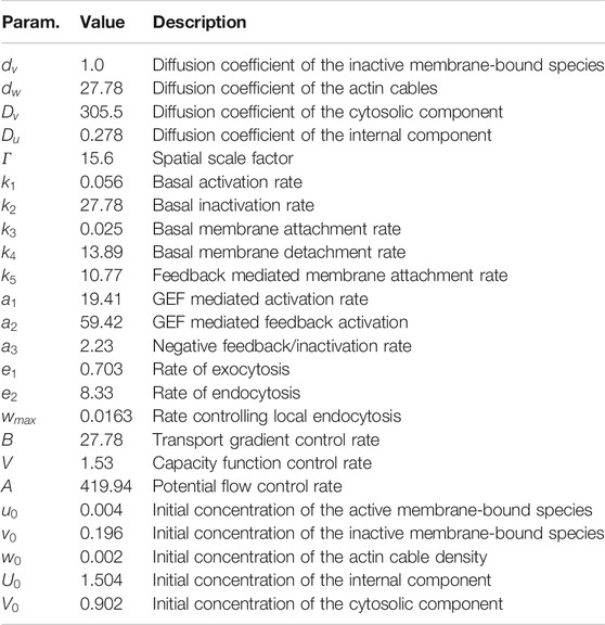
TABLE 1. Parameters used for computations of the generic system. Variables and constants used for numerical simulations of the nondimensionalized system (1) considering reaction kinetics derived in Ref. 6 are shown.

4.2 Actin-Mediated Cell Polarization

In the following, we confirm the results of the linear stability analysis performed in the previous section. In particular, we compare simulations of the full system (1) and the simplified system (3), which was used in the analysis. As we assumed a well-mixed pool, the effect of exocytosis and endocytosis were assumed to dominate over the actual vesicle transport along actin cables. To simulate transport via exocytosis and endocytosis, we define

$h\left(u,w,U\right)=e_{1}wU-e_2\left(1-\delta \left(w\right)\frac{w}{w_{max}}\right)u.$

In the simplified (well-mixed) case, the transport to the membrane is slower, due to the nearly homogeneous distribution of U. Thus, we had to increase $e_1$ and decrease $e_2$ to obtain similar results as for the full system, where molecules are actively transported. These rates are chosen such that we obtain similar ratios between internal and membrane components as before. We set $e_1=84.3$ and $e_2=4.167$.

In all computations, we use functions $f,g$ as given in (22) and (23), respectively. We use initial concentrations and parameters as given in Table 1.

We numerically solve system (3) for the different cases to investigate its behavior.

The most interesting outcome of the stability analysis is the fact that the conditions determining instability are completely independent of the diffusion parameter $d_w$. This implies that the only requirement on $d_w$ is that it must be nonzero. In this case, the capacity function $c\left(u\right)$ determines whether the system is stable against small perturbations or not. We further call this capacity-driven instability.

Figure 1 shows the development of u in time for distinct values of $d_w$. We observe that even for large changes of $d_w$, provided that $d_w\ne 0$, the system is always unstable and tends to form a polarized patch. It becomes clear that the capacity function $c\left(u\right)$ as well as $w^{\text{*}}$ determines the stability behavior. The constant $d_w$ only changes the temporal dynamic of polarization (see Figure 1). For reduced rates, the maximum value of u is reached much later. It can be shown that even for $d_w\ll 1$, the system is still able to form a polarized patch, albeit after a very long time ($t>30$).

FIGURE 1

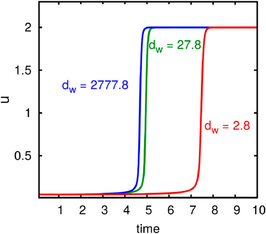
FIGURE 1. Computational results demonstrating the influence of the diffusion constant for actin cable movement on the polarization process. The development of the maximum of u in time is shown. Computations with different rates for $d_w$ are compared.

As mentioned in Remark 2.1, the model is mass conservative. Our numerical model adequately reproduce this behavior due to the use of a locally mass conservative method. The evolution of mass of the different components $u,v,U,V$ as well as the total mass is visualized in Figure 2.

FIGURE 2

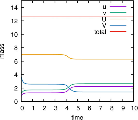
FIGURE 2. Computational validation of mass conservation. Temporal evolution of mass of components $u,v,U,V$, and the total mass. As the numerical scheme is based on a locally mass conservative CVFE method, the conservation of mass property of the model is also fulfilled in the numerical simulations.

Another result of the stability analysis is the fact that we may observe polarization, even if $V=0$ or $U=0$. From Figure 3, we see that the generic system is able to represent these cases. Even in the absence of a cytosolic exchange or a transport mechanism, the system becomes unstable and forms a polarized cluster.

FIGURE 3

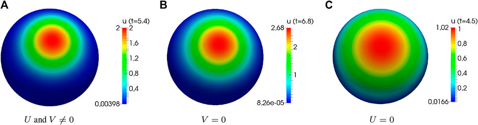
FIGURE 3. Numerical simulations of the generic system showing distinct cases of instability. Computational results of system (3) showing distinct cases of instability ($e_1=84.3$, $e_2=4.167$). (A) The internal as well as cytosolic component is nonzero. A small initial perturbation leads to an instability inducing a polarized patch. (B) Without the cytosolic component, a capacity-driven instability causes peak formation. (C) Even if the internal component is zero, the cell is still able to become unstable.

The requirement $D_u\gg 1$ yields that $D_v$ must not be very large to ensure instability. We have seen that even in the case $D_v\approx 1$, the instability conditions may be satisfied. Our numerical simulations confirm these results. Figure 4 illustrates capacity-driven polarization for the system (3), where $D_v=1$.

FIGURE 4

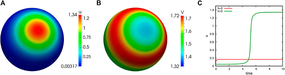
FIGURE 4. Numerical simulations of the generic system showing capacity-driven instability. Computational results of system (3) with $e_1=15$, $e_2=0.2$ are shown The internal as well as cytosolic component is nonzero. Computational results of the system (3) with drastically reduced diffusion constant $D_V=1$. (A) Concentration u after time $t=10$ ($h\ne 0$). (B) Concentration V after time $t=10$ ($h\ne 0$). (C) Temporal development of u. Computational results are shown for the system with and without consideration of transport.

4.3 Cell Shape Influences Transport-Driven Cell Polarization

Active transport of molecules plays a significant role in many cell types. For example, in the fission yeast, neurons and the Caenorhabditis elegans zygote microtubules may mediate the transport of important regulators of cell polarization and in this way ensure its correct location [19, 26, 30]. Therefore, our modeling approach can be used to investigate polarization for a range of different cell types with distinct shapes.

In order to understand the influence of the cell shape on polarization, we simulate the system for different three-dimensional model geometries. We employ a random signal to drive the cell out of its uniform state. The results are shown in Figure 5. In all cases, we obtain an enhanced peak of the nondimensional concentration u.

FIGURE 5

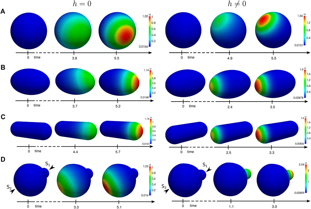
FIGURE 5. Numerical simulations of the generic system applied to different geometries. Simulation results at different time steps with functions (22), without (left) and with (right) the proposed active molecule transport. A spatial noise signal applied to the initial uniform state $u_0$(A–C) results in cluster formation. In (D), we applied an excitation for $\text{Δ}t=0.69$ with two equal stimuli with $s_1=s_2=0.1$. For geometries (A–D), we observe an enhanced peak due to active transport. In the case of two stimuli (D), it can even change the polarization site toward the protrusion.

One observes that transport-mediated polarization is significantly accelerated in nonspherical cells. In this case, the gradient increases or decreases with the length or broadness of the shape, respectively. Regarding the polarity direction, our results show that transport can change the spatial location of the polarized patch. This becomes particularly obvious in Figure 5D which shows polarity in a cell that features a small bud. In this case, we excite the cell from its homogeneous state by a signal comprising of two stimuli $S_1$ and $S_2$ of the same intensity. The signals are imposed on opposite sides of the cell surface, one located at the protrusion. Depending on the presence of transport, different patterns are obtained. In the presence of active transport, a peak forms at the bud, without u clusters at the opposite side. The influence of protrusions on diffusion-driven polarization in a cell has already been studied in Ref. 10. Their results have shown that protrusions locally limit molecule aggregations. Diffusive transport into the protrusion is slightly hindered so that the cytosolic concentration decreases faster in this region. As a result, the cluster emerges at another location. Interestingly, our results demonstrate that for sufficiently high rates of active transport, this kind of “bottle neck” can be compensated, and the cluster forms at the protrusion.

Depending on the particular rates, feedback strength, and the interplay between transport and reaction kinetics, transport can either enhance or disturb polarity. For some choices, it even perturbs the system so strongly that it is no longer capable of polarization.

4.4 Influence of Internal Components on Cell Polarization

Cells contain many different cell components of distinct shape and size like for instance the nucleus, the Golgi, or the endoplasmic reticulum. All these structures serve as a kind of diffusion and transport barrier within the cell. In this way, the spatial position of organelles can influence signaling pathways, including the accumulation of polarization molecules.

How internal barriers control diffusion-driven cell polarization has already been investigated in Ref. 10. The results have demonstrated that the cluster formation close to organelles is very unlikely. Diffusion-driven polarization mostly occurred in the neighborhood of large organelles, but not behind them. The local accumulation of substances at the opposite side of protrusions or in regions with low curvature is more likely [10].

In order to investigate whether active transport alters the results, we perform similar computational experiments. We consider the two-dimensional case, where the cell is characterized by a circle. Organelles are modeled by elliptic or circular shapes placed in the cell interior. The results are shown in Figure 6. Again, we excite the cell from its homogeneous state by a signal comprising two stimuli $S_1$ and $S_2$ of the same intensity. Whereas one signal is located near the organelles, the other is placed at the opposite side.

FIGURE 6

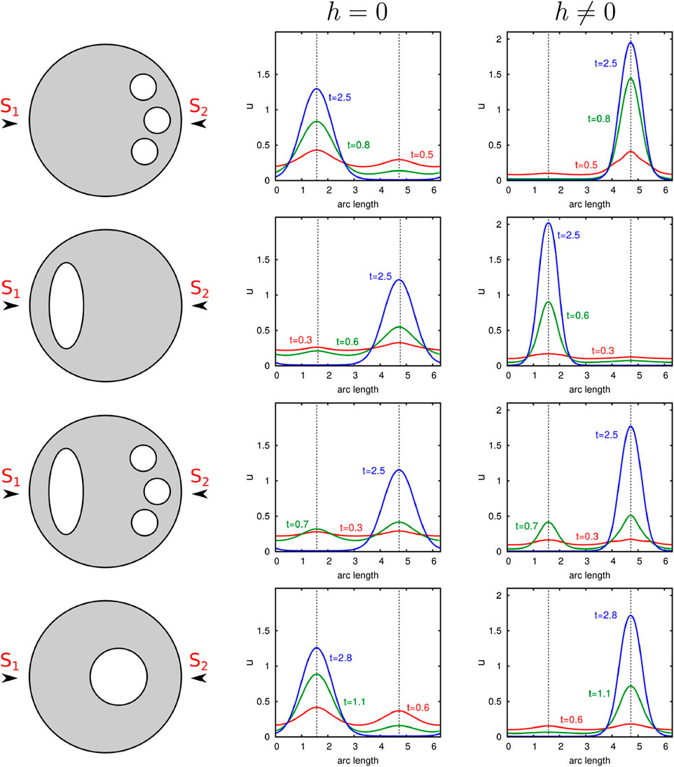
FIGURE 6. Illustration of the influence of internal barriers on cell polarization. Computational results of our nondimensional model with and without transport are presented. Organelles which are represented by circles or ellipses are placed at distinct positions in the cell. Computations with two equal stimuli exciting the initial uniform state $u_0$ with $s_1=s_2=0.2$ for $\text{Δ}t=0.69$ are shown.

Without consideration of transport effects, we obtain similar results as presented in Ref. 10. The organelles near the surface negatively affect cluster formation at this site. Contrarily, we see that under consideration of active molecule transport, the polar cluster forms behind the internal component. In this case, organelles support a nearby spatial location of the polarity patch.

As mentioned before, protrusions positively influence transport-mediated polarization too. This raises the question of how polarity behaves in cells exhibiting both a complex shape and internal barriers. Figure 7 illustrates this interplay. It becomes clear that since protrusions as well as diffusion barriers can promote polarization, the localization of organelles next to protrusions strongly enhances polarity. Conversely, we see that an opposed position leads to a competing situation. As long as the organelle is sufficiently far away from the surface and centrally located, the cluster still forms at the bud. In contrast, when the organelle is placed near the membrane, but opposed to the protrusion, we obtain polarization behind the organelle. Only a very strong stimulus at the protrusion reverses the outcome. This is demonstrated by the last computational experiment illustrated in Figure 7, where the cell is excited at the bud tip with a signal $S_1$ of strength $s_1=0.33$.

FIGURE 7

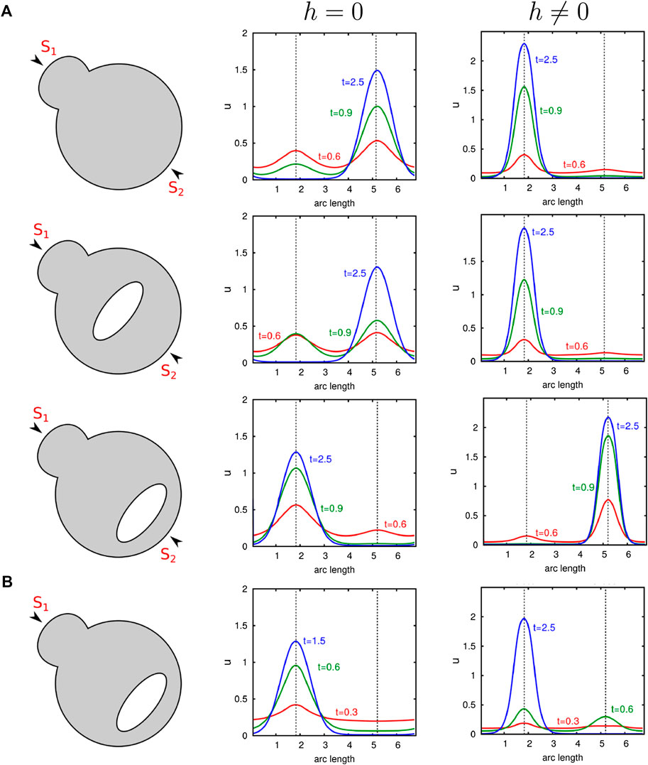
FIGURE 7. Comparison of the influence of organelles as well as the cell shape on diffusion- and transport-mediated polarization. Numerical simulations of our nondimensional model with and without transport are presented. A large organelle which is represented by an ellipse is placed at distinct positions in a cell exhibiting a small protrusion. (A) Simulations with two equal stimuli exciting the initial uniform state u with $s_1=s_2=0.2$ for $\text{Δ}t=0.69$ are illustrated. Cluster formation either occurs behind the organelle or, if the barrier is sufficiently far away from the surface, at the protrusion. (B) Only a strong stimulus $s_1=0.33$ can reverse this feature (bottom computation).

5 Discussion

Based on a complex bulk-surface reaction–diffusion–advection system for cell polarization proposed in Ref. 6, in this work, we have introduced a generic approach for the simulation of transport-mediated cell polarization. We performed numerical simulations with distinct cell geometries and cell types, and compared the results to those found in the literature. Since our main interest was to analyze the conditions leading to cluster formation, we further performed a linear stability analysis considering a spherical cell.

The results have shown that vesicular transport may not only influence the robustness, shape, and intensity of the polar cluster but also its spatial location. Particularly, in cells with complex shapes, we observed different patterns between simulations with and without active molecule transport. Here, protrusions and narrower domains differently affected symmetry breaking. Whereas complex shapes rather inhibit diffusion-driven symmetry breaking, transport-mediated polarization can be enhanced under these circumstances.

However, cells are able to robustly polarize at sites of complex protrusions. For example, the tip of the future axon is strongly polarized during neuronal development. These findings suggest that, especially in nonspherical cells, active transport may be required to ensure the correct location of the polarized patch, which is in line with previous finding in Ref. 7.

Based on a complex bulk-surface system for the simulation of cell polarization, we have presented a reduced generic system of bulk-surface reaction–diffusion–advection equations. Our main interest here was to analyze the conditions leading to pattern formation. Therefore, using a spherical cell, we applied a linear stability analysis to a simplified system composing three surface quantities and two bulk concentrations. Our results have demonstrated that two different main mechanisms lead to symmetry breaking. The first one is related to a classical diffusion-driven instability studied in Refs. 22 and 23. The second mechanism is controlled by a capacity-dependent inhomogeneous diffusion of the transport triggering factor. Such dependence has the capability to induce a positive feedback leading to spatial patterns.

However, we have restricted our analytical and numerical studies to stationary domains. In many cases, biological processes induce the development of cell shapes. Thus, the consideration of surfaces which evolve continuously in time would be of great interest. But this implies a more complicated modeling, analysis, and simulation of the coupled system and could be focus of further studies. The results have shown that vesicular transport may not only influence the robustness, shape, and intensity of the polar cluster but also its spatial location. Particularly, in cells with complex shapes, we observed different patterns between simulations with and without active molecule transport. Here, protrusions and narrower domains differently affected symmetry breaking. Whereas complex shapes rather inhibit diffusion-driven symmetry breaking, transport-mediated polarization can be enhanced under these circumstances.

Another outcome of the computational results is the distinct role of organelles. Whereas internal barriers inhibit diffusion-driven polarization behind them, active transport is able to overcome this negative feedback to facilitate polarity next to organelles. The influence of internal components on the direction of cluster formation has already been shown by biological experiments. To give an example, studies with the fission yeast have demonstrated that the position of the interphase nucleus dictates the future site of cell division [5]. These findings together with our results emphasize that it is of particular importance to consider spatial aspects in the mathematical study of cell polarization. As a consequence, to investigate such biological processes in greater detail, the application of more complex mathematical models, including coupling bulk-surface PDEs, must take on greater significance.

Unfortunately, with growing complexity, the analysis of mathematical models becomes increasingly challenging. To enable a linear stability analysis, we continued with a reduction of the generic approach given by reaction–diffusion–advection equations to a minimal coupled bulk-surface reaction–diffusion–transport system. The stability analysis has shown that the reduced generic system is able to generate spatial patterns under certain conditions. These conditions confirm that the transport process derived in this work can increase the robustness of the system. The reason is that two distinct mechanisms act in parallel to generate symmetry breaking. These can explain polarization in $\text{Δ}rdi1$ and LatA-treated cells. Treating wild-type yeast cells with latrunculin A (LatA) removes the actin-dependent recycling pathway, while $\text{Δ}rdi1$ denotes cells with removed GDI, which both can establish polarization [27].

The first one relates to a classical Turing instability which requires a large difference in the cytosolic and membrane diffusion coefficient. Even if there is no transport of molecules from and to an internal compartment, this mechanism is able to achieve polarization. Since this case has already been analyzed in detail, at this point, we refer the reader to Ref. 23.

The second mechanism is based on a capacity function that regulates the concentration of the component driving transport. Under certain conditions, this mechanism can induce symmetry breaking, even if the cytosolic exchange is blocked. Hence, this case explains symmetry breaking in cells lacking the cytosolic component. In this case, $d_w\ne 0$, the capacity function $c\left(u\right)$ together with the homogeneous state of w entirely determines the stability behavior.

By the performance of numerical simulations, we finally confirmed the results of the stability analysis and demonstrated that our model is able to show the different cases derived. Furthermore, we have shown that this capacity-driven instability also generates pattern when the cytosolic and membrane diffusion rates are equal. For that reason, and since the diffusion constant $d_w$ has no essential impact on the stability of the system, we assert that this instability mechanism distinguishes from the Turing-type instability.

Data Availability Statement

The raw data supporting the conclusions of this article will be made available by the authors, without undue reservation.

Author Contributions

NE contributed to the modeling, analysis, numerical simulations, and preparation of the manuscript. CE contributed to the modeling and numerical simulations, guided the research, and contributed to the preparation of the manuscript.

Funding

The content of this manuscript has been published as part of the thesis of [6]. NE was supported by the Deutsche Forschungsgemeinschaft (DFG, German Research Foundation) under Germany’s Excellence Strategy EXC 1003, Cells in Motion, CiM, Münster. CE was supported by the Deutsche Forschungsgemeinschaft (DFG, German Research Foundation) under Germany’s Excellence Strategy EXC 2044-390685587, Mathematics Münster: Dynamics–Geometry–Structure.

Conflict of Interest

The authors declare that the research was conducted in the absence of any commercial or financial relationships that could be construed as a potential conflict of interest.

Supplementary Material

The Supplementary Material for this article can be found online at: https://www.frontiersin.org/articles/10.3389/fams.2020.570036/full#supplementary-material

References

1. Ayscough, KR, Stryker, J, Pokala, N, Sanders, M, Crews, P, and Drubin, DG. High rates of actin filament turnover in budding yeast and roles for actin in establishment and maintenance of cell polarity revealed using the actin inhibitor latrunculin-A. J Cell Biol (1997). 137:399–416. doi: 10.1083/jcb.137.2.399.

CrossRef Full Text | Google Scholar

2. Bastian, P, Blatt, M, Dedner, A, Engwer, C, Klöfkorn, R, Kornhuber, R, et al. A generic grid interface for parallel and adaptive scientific computing. part II: implementation and tests in DUNE. Computing (2008). 82:121–38. doi: 10.1007/s00607-008-0004-9.

CrossRef Full Text | Google Scholar

3. Bastian, P, Blatt, M, Dedner, A, Engwer, C, Klöfkorn, R, Ohlberger, M, et al. A generic grid interface for parallel and adaptive scientific computing. part I: abstract framework. Computing (2008b). 82:103–19. doi: 10.1007/s00607-008-0003-x

CrossRef Full Text | Google Scholar

4. Bastian, P, Heimann, F, and Marnach, S. Generic implementation of finite element methods in the distributed and unified numerics environment. Kybernetik (2010). 46, 294–315.

Google Scholar

5. Daga, RR, and Chang, F. Dynamic positioning of the fission yeast cell division plane. Proc Natl Acad Sci USA (2005). 102, 8228–32. doi: 10.1073/pnas.0409021102

CrossRef Full Text | Google Scholar

6. Emken, N. A coupled bulk-surface reaction-diffusion-advection model for cell polarization. [PhD thesis]. Münster University of Münster (2016).

Google Scholar

7. Emken, N, Püschel, A, and Burger, M. Mathematical modelling of polarizing gtpases in developing axons. arXiv preprint arXiv:1204.5725 (2012).

Google Scholar

8. Etienne-Manneville, S, and Hall, A. Rho gtpases in cell biology. Nature (2002). 420, 629–35. doi: 10.1038/nature01148.

CrossRef Full Text | Google Scholar

9. Freisinger, T, Klünder, B, Johnson, J, Müller, N, Pichler, G, Beck, G, et al. Establishment of a robust single axis of cell polarity by coupling multiple positive feedback loops. Nat Commun (2013). 4, 1–11. doi: 10.1038/ncomms2795

CrossRef Full Text | Google Scholar

10. Giese, W, Eigel, M, Westerheide, S, Engwer, C, and Klipp, E. Influence of cell shape, inhomogeneities and diffusion barriers in cell polarization models. Phys Biol (2015). 12, 066014. doi: 10.1088/1478-3975/12/6/066014

CrossRef Full Text | Google Scholar

11. Goryachev, AB, and Pokhilko, AV. Dynamics of cdc42 network embodies a turing-type mechanism of yeast cell polarity. FEBS Lett (2008). 582, 1437–43. doi: 10.1016/j.febslet.2008.03.029

CrossRef Full Text | Google Scholar

12. Howell, AS, Savage, NS, Johnson, SA, Bose, I, Wagner, AW, Zyla, TR, et al. Singularity in polarization: rewiring yeast cells to make two buds. Cell (2009). 139, 731–43. doi: 10.1016/j.cell.2009.10.024

CrossRef Full Text | Google Scholar

13. Johnson, JM, Jin, M, and Lew, DJ. Symmetry breaking and the establishment of cell polarity in budding yeast. Curr Opin Genet Dev (2011). 21, 740–6. doi: 10.1016/j.gde.2011.09.007

CrossRef Full Text | Google Scholar

14. Klünder, B, Freisinger, T, Wedlich-Söldner, R, and Frey, E. Gdi-mediated cell polarization in yeast provides precise spatial and temporal control of cdc42 signaling. PLoS Comput Biol (2013). 9:e1003396. doi: 10.1371/journal.pcbi.1003396.

CrossRef Full Text | Google Scholar

15. Knabner, P, and Angerman, L. Numerical methods for elliptic and parabolic partial differential equations. New York, NY: Springer (2003).

Google Scholar

16. Krauss, G, Schönbrunner, N, and Cooper, J. Biochemistry of signal transduction and regulation. (Bayreuth: Wiley Online Library), Vol. 3 (2003).

Google Scholar

17. Layton, AT, Savage, NS, Howell, AS, Carroll, SY, Drubin, DG, and Lew, DJ. Modeling vesicle traffic reveals unexpected consequences for cdc42p-mediated polarity establishment. Curr Biol (2011). 21, 184–94. doi: 10.1016/j.cub.2011.01.012

CrossRef Full Text | Google Scholar

18. Madzvamuse, A, Chung, AHW, and Venkataraman, C. Stability analysis and simulations of coupled bulk-surface reaction-diffusion systems. Proc. R. Soc. A (2015). 471, 20140546. doi: 10.1098/rspa.2014.0546

CrossRef Full Text | Google Scholar

19. Mata, J, and Nurse, P. tea1 and the microtubular cytoskeleton are important for generating global spatial order within the fission yeast cell. Cell (1997). 89, 939–49. doi: 10.1016/s0092-8674(00)80279-2

CrossRef Full Text | Google Scholar

20. Müthing, S. A flexible framework for multi physics and multi domain PDE simulations. [PhD thesis]. Institut für Parallele und Verteilte Systeme der Stuttgart: Universität Stuttgart (2015). doi: 10.18419/opus-3620

CrossRef Full Text | Google Scholar

21. Rätz, A. Turing-type instabilities in bulk-surface reaction-diffusion systems. J Comput Appl Math (2015). 289:142–52. doi: 10.1016/j.cam.2015.02.050

CrossRef Full Text | Google Scholar

22. Rätz, A, and Röger, M. Turing instabilities in a mathematical model for signaling networks. J Math Biol (2012). 65:1215–44. doi: 10.1007/s00285-011-0495-4

CrossRef Full Text | Google Scholar

23. Rätz, A, and Röger, M. Symmetry breaking in a bulk-surface reaction-diffusion model for signalling networks. Nonlinearity (2014). 27:1805–27. doi: 10.1088/0951-7715/27/8/1805

CrossRef Full Text | Google Scholar

24. Sagot, I, Klee, SK, and Pellman, D. Yeast formins regulate cell polarity by controlling the assembly of actin cables. Nat Cell Biol (2002). 4:42–50. doi: 10.1038/ncb719

CrossRef Full Text | Google Scholar

25. Savage, NS, Layton, AT, and Lew, DJ. Mechanistic mathematical model of polarity in yeast. Mol Biol Cell (2012). 23:1998–2013. doi: 10.1091/mbc.e11-10-0837

CrossRef Full Text | Google Scholar

26. Siegrist, SE, and Doe, CQ. Microtubule-induced cortical cell polarity. Genes Dev (2007). 21:483–96. doi: 10.1101/gad.1511207

CrossRef Full Text | Google Scholar

27. Slaughter, BD, Das, A, Schwartz, JW, Rubinstein, B, and Li, R. Dual modes of cdc42 recycling fine-tune polarized morphogenesis. Dev Cell (2009). 17:823–35. doi: 10.1016/j.devcel.2009.10.022

CrossRef Full Text | Google Scholar

28. Slaughter, BD, Smith, SE, and Li, R. Symmetry breaking in the life cycle of the budding yeast. Cold Spring Harb Perspect Biol (2009). 1:a003384. doi: 10.1101/cshperspect.a003384

CrossRef Full Text | Google Scholar

29. Symons, MH. Rho GTPases. Molecular biology intelligence unit. Springer (2004).

Google Scholar

30. Tahirovic, S, and Bradke, F. Neuronal polarity. Cold Spring Harb Perspect Biol (2009). 1:a001644. doi: 10.1101/cshperspect.a001644

CrossRef Full Text | Google Scholar

31. Tanos, B, and Rodriguez-Boulan, E. The epithelial polarity program: machineries involved and their hijacking by cancer. Oncogene (2008). 27:6939–57. doi: 10.1038/onc.2008.345

CrossRef Full Text | Google Scholar

32. Wedlich-Soldner, R, Altschuler, S, Wu, L, and Li, R. Spontaneous cell polarization through actomyosin-based delivery of the cdc42 gtpase. Science (2003). 299:1231–5. doi: 10.1126/science.1080944

CrossRef Full Text | Google Scholar

33. Wedlich-Söldner, R, Wai, SC, Schmidt, T, and Li, R. Robust cell polarity is a dynamic state established by coupling transport and GTPase signaling. J Cell Biol (2004). 166:889–900. doi: 10.1083/jcb.200405061

CrossRef Full Text | Google Scholar