Mathematical modeling and simulation of SEIR model for COVID-19 outbreak: A case study of Trivandrum

M, Aakash; C, Gunasundari; Al-Mdallal, Qasem M.

doi:10.3389/fams.2023.1124897

ORIGINAL RESEARCH article

Front. Appl. Math. Stat., 15 February 2023
Sec. Mathematics of Computation and Data Science
Volume 9 - 2023 | https://doi.org/10.3389/fams.2023.1124897

Mathematical modeling and simulation of SEIR model for COVID-19 outbreak: A case study of Trivandrum

Aakash M¹

Gunasundari C¹

Qasem M. Al-Mdallal²^*

¹Department of Mathematics, Faculty of Engineering and Technology, SRM Institute of Science and Technology, Chengalpattu, India
²Department of Mathematical Sciences, UAE University, Al Ain, United Arab Emirates

In this study, we formulated a mathematical model of COVID-19 with the effects of partially and fully vaccinated individuals. Here, the purpose of this study is to solve the model using some numerical methods. It is complex to solve four equations of the SEIR model, so we introduce the Euler and the fourth-order Runge–Kutta method to solve the model. These two methods are efficient and practically well suited for solving initial value problems. Therefore, we formulated a simple nonlinear SEIR model with the incorporation of partially and fully vaccinated parameters. Then, we try to solve our model by transforming our equations into the Euler and Runge–Kutta methods. Here, we not only study the comparison of these two methods, also found out the differences in solutions between the two methods. Furthermore, to make our model more realistic, we considered the capital of Kerala, Trivandrum city for the simulation. We used MATLAB software for simulation purpose. At last, we discuss the numerical comparison between these two methods with real world data.

1. Introduction

Coronaviruses are a large family of viruses that can infect both animals and humans with humans being seriously affected. Several coronaviruses have been linked to respiratory infections in humans, ranging from the common cold to more serious illnesses including the Middle East respiratory syndrome (MERS) and severe acute respiratory syndrome (SARS). Coronavirus disease 2019 (COVID-19) is caused by the most recent forms of coronavirus. For the past 2 years, people all over the world have been affected by COVID-19, which is the fifth pandemic after the 1918 Spanish flu (H1N1) pandemic, followed by the 1957 Asian flu (H2N2), the 1968 Hong Kong flu (H3N2), and the 2009 Swine flu pandemic (H1N1) pandemics [1]. COVID-19 is an infectious disease caused by various strains of coronavirus. It is the seventh member of the coronavirus family. This pandemic has seen a surge of patients with acute respiratory distress syndrome (ARDS) in intensive care units across the globe [2]. We study the outbreak in the capital of Kerala, Trivandrum city, which is also called Thiruvananthapuram. Till 30 December, 2021, this city has recorded 5,07,748 COVID-19-positive cases, out of which 4,99,009 cases have recovered and 6,257 have deceased. This pandemic not only affects the population but also affects the economics around the world [3]. So, by using the mathematical model, we can find the transmission of disease into the population. This provides us with a better understanding of how to deal with the current circumstance. It plays a powerful component in studying the dynamics of the spread of infectious diseases such as Ebola virus disease [4]. Disease in the ecosystem has become a popular research topic, and communicable disease has become a vital aspect of human population monitoring [5]. It makes us understand the dynamics of the disease and provides prediction about the spread of the disease. Haneen et al. [6] have constructed a simple and effective numerical algorithm that provides approximate solutions to complicated problems, especially the modeling of real-world phenomena [6]. Many authors use the utilized fractional differential problem, which is a modern mathematical formation model [7, 8]. According to Kolokolnikov and Iron [9], the SEIR model is a simple dynamic model that describes the spread of the disease between populations [9]. Similarly, some of the researchers used the same SEIR approach in Xu et al. [10] and Peng et al. [11]. Some SEIR approaches have been done in Hurit et al. [12] and Alsakaji et al. [13]. Here, the author formulated and solved the model using the Euler method, the Runge–Kutta method, and Heun's method. Therefore, these mathematical models give valuable information, ideas, and control measures to the public as well as the government.

In this study, we are going to formulate a nonlinear ordinary differential equation. Here, we are going to solve the proposed model by using numerical methods. Therefore, we approach the Euler and Runge–Kutta methods. In these two methods, the values of y are calculated by short steps ahead of equal interval h of the independent variable x [14].

Now, the general form of the Euler method can be written as follows:

\begin{array}{l} y_{n + 1} = y_{n} + h f (x_{n}, y_{n}), where n varies from 0,1,2,.. . & (1) \end{array}

In the case of the fourth order Runge–Kutta method, we have,

\begin{array}{l} y_{n + 1} = y_{n} + \frac{1}{6} (K_{1} + 2 K_{2} + 2 K_{3} + K 4), where n varies from 0,1,2,.. . & (2) \end{array}

where

\begin{array}{l} K_{1} = h f (t_{n}, y_{n}), \\ K_{2} = h f (t_{n} + \frac{1}{2} h, y_{n} + \frac{1}{2} K_{1}), \\ K_{3} = h f (t_{n} + \frac{1}{2} h, y_{n} + \frac{1}{2} K_{2}), \\ K_{4} = h f (t_{n} + h, y_{n} + K_{3}) . \end{array}

Here, in our proposed study, we formulated a COVID-19 model by incorporating the effects of partially vaccinated and fully vaccinated individuals at Trivandrum city. We tried to solve our model with various numerical techniques by using the Euler and Runge–Kutta methods. We have transformed our whole system into the Euler and fourth order Runge–Kutta equations by using general iterative formulas, and the solution is obtained by using MATLAB software.

Our study is organized as follows. The next section presents the formulation of the COVID-19 model, followed by the transformation of our SEIR model into the Euler and fourth order Runge–Kutta equations. Section 3 deals with the applications and solutions of both proposed methods, and Section 4 is devoted to results and discussion. In that, simulation results and absolute differences between both methods are presented. Furthermore, comparison and curve fitting are done with real-world data. The study ends with a brief conclusion in Section 5.

2. Methodology

2.1. Formulation of the SEIR model

We consider the human population, which we split into four subpopulations, namely, Susceptible individuals S(t), Exposed individuals E(t), Infected individuals I(t), and Recovered individuals R(t). To build our system, the following assumptions have been made: Individuals are recruited in the region at a fixed rate A and join the susceptible compartment. The susceptible population become exposed to the infection when an infected individual comes in contact at the rate α. Furthermore, we assume that the exposed population become infected at a constant rate δ > 0. Here, we have incorporated partially vaccinated population V_p and fully vaccinated population V_f into the model to make it more realistic. Therefore, those who are partially vaccinated may get exposed, and the fully vaccinated individuals directly move to the recovery compartment. Other than vaccinated individuals, the remaining infected individuals recovered due to treatment at the rate γ. By using these assumptions, a model is framed, which is described as follows:

\begin{array}{l} \frac{d S}{d t} = A - α S I - μ S - V_{p} S - V_{f} S, \\ \frac{d E}{d t} = α S I - μ E - δ E + V_{p} S, \\ \frac{d I}{d t} = δ E - μ I - μ_{1} I - γ I, \\ \frac{d R}{d t} = V_{f} S + γ I - μ R . & (3) \end{array}

Here, N = S(t) + E(t) + I(t) + R(t) is the total population. Tables 1–3 gives the description of the parameters, initial values of the variables and values of the parameter respectively.

TABLE 1

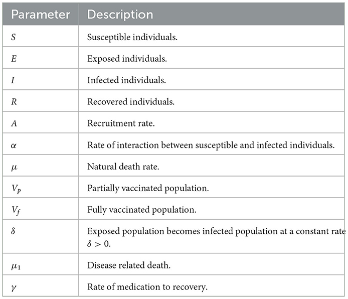
Table 1. Description of parameters.

TABLE 2

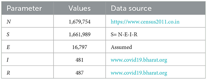
Table 2. Initial values of variables.

TABLE 3

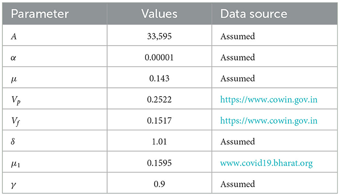
Table 3. Values of parameters.

2.2. Transformation of Euler equations for our SEIR model

For our model, the dependent variables are S, E, I, and R. So, from the general iterative formula for the Euler method, S(T), E(t), I(t), and R(t) can be modified as follows:

\begin{array}{l} S_{n + 1} = S_{n} + Δ t (A - α S_{n} I_{n} - μ S_{n} - V_{p} S_{n} - V_{f} S_{n}), \\ E_{n + 1} = E_{n} + Δ t (α S_{n} I_{n} - μ E_{n} - δ E_{n} + V_{p} S_{n}), \\ I_{n + 1} = I_{n} + Δ t (δ E_{n} - μ I_{n} - μ_{1} I_{n} - γ I_{n}), \\ R_{n + 1} = R_{n} + Δ t (V_{f} S_{n} + γ I_{n} - μ R_{n}) . & (4) \end{array}

From these iterative formulas, we have calculated the values for 55 days from 1 January 2022 to 24 February 2022 at Trivandrum city. But before this, we should fix the initial values for variables and parameters, which is discussed in the next section.

2.3. Transformation of Runge–Kutta equations for our SEIR model

From the general iterative formula for the fourth order Runge–Kutta method, S(T), E(t), I(t), and R(t) can be modified as follows:

\begin{array}{l} K_{1}^{S} = f (t_{n}, S_{n}, I_{n}) \\ = A - α S_{n} I_{n} - μ S_{n} - V_{p} S_{n} - V_{f} S_{n} . \\ K_{2}^{S} = f (t_{n} + \frac{Δ t}{2}, S_{n} + \frac{Δ t}{2} K_{1}^{S}, I_{n} + \frac{Δ t}{2} K_{1}^{I}) \\ = A - α (S_{n} + K_{1}^{S} \frac{Δ t}{2}) (I_{n} + K_{1}^{I} \frac{Δ t}{2}) - μ (S_{n} + K_{1}^{S} \frac{Δ t}{2}) \\ - V_{p} (S_{n} + K_{1}^{S} \frac{Δ t}{2}) - V_{f} (S_{n} + K_{1}^{S} \frac{Δ t}{2}) . \\ K_{3}^{S} = f (t_{n} + \frac{Δ t}{2}, S_{n} + \frac{Δ t}{2} K_{2}^{S}, I_{n} + \frac{Δ t}{2} K_{2}^{I}) \\ = A - α (S_{n} + K_{2}^{S} \frac{Δ t}{2}) (I_{n} + K_{2}^{I} \frac{Δ t}{2}) - μ (S_{n} + K_{2}^{S} \frac{Δ t}{2}) \\ - V_{p} (S_{n} + K_{2}^{S} \frac{Δ t}{2}) - V_{f} (S_{n} + K_{2}^{S} \frac{Δ t}{2}) . \\ K_{4}^{S} = f (t_{n} + Δ t, S_{n} + Δ t K_{3}^{S}, I_{n} + Δ t K_{3}^{I}) \\ = A - α (S_{n} + K_{3}^{S} Δ t) (I_{n} + K_{3}^{I} Δ t) - μ (S_{n} + K_{3}^{S} Δ t) \\ - V_{p} (S_{n} + K_{3}^{S} Δ t) - V_{f} (S_{n} + K_{3}^{S} Δ t) . \end{array}

\begin{array}{l} K_{1}^{E} = f (t_{n}, S_{n}, E_{n}, I_{n}) \\ = α S_{n} I_{n} - μ E_{n} - δ E_{n} + V_{p} S_{n} . \\ K_{2}^{E} = f (t_{n} + \frac{Δ t}{2}, S_{n} + \frac{Δ t}{2} K_{1}^{S}, E_{n} + \frac{Δ t}{2} K_{1}^{E}, I_{n} + \frac{Δ t}{2} K_{1}^{I}) \\ = α (S_{n} + K_{1}^{S} \frac{Δ t}{2}) (I_{n} + K_{1}^{I} \frac{Δ t}{2}) - μ (E_{n} + K_{1}^{E} \frac{Δ t}{2}) \\ - δ (E_{n} + K_{1}^{E} \frac{Δ t}{2}) + V_{p} (S_{n} + K_{1}^{S} \frac{Δ t}{2}) . \\ K_{3}^{E} = f (t_{n} + \frac{Δ t}{2}, S_{n} + \frac{Δ t}{2} K_{2}^{S}, E_{n} + \frac{Δ t}{2} K_{2}^{E}, I_{n} + \frac{Δ t}{2} K_{2}^{I}) \\ = α (S_{n} + K_{2}^{S} \frac{Δ t}{2}) (I_{n} + K_{2}^{I} \frac{Δ t}{2}) - μ (E_{n} + K_{2}^{E} \frac{Δ t}{2}) \\ - δ (E_{n} + K_{2}^{E} \frac{Δ t}{2}) + V_{p} (S_{n} + K_{2}^{S} \frac{Δ t}{2}) . \\ K_{4}^{E} = f (t_{n} + Δ t, S_{n} + Δ t K_{3}^{S}, E_{n} + Δ t K_{3}^{E}, I_{n} + Δ t K_{3}^{I}) \\ = α (S_{n} + K_{3}^{S} Δ t) (I_{n} + K_{3}^{I} Δ t) - μ (E_{n} + K_{3}^{E} Δ t) \\ - δ (E_{n} + K_{3}^{E} Δ t) + V_{p} (S_{n} + K_{3}^{S} Δ t) . \end{array}

\begin{array}{l} K_{1}^{I} = f (t_{n}, E_{n}, I_{n}) \\ = δ E_{n} - μ I_{n} - μ_{1} I_{n} - γ I_{n} . \\ K_{2}^{I} = f (t_{n} + \frac{Δ t}{2}, E_{n} + \frac{Δ t}{2} K_{1}^{E}, I_{n} + \frac{Δ t}{2} K_{1}^{I}) \\ = δ (E_{n} + K_{1}^{E} \frac{Δ t}{2}) - μ (I_{n} + K_{1}^{I} \frac{Δ t}{2}) - μ_{1} (I_{n} + K_{1}^{I} \frac{Δ t}{2}) \\ - γ (I_{n} + K_{1}^{I} \frac{Δ t}{2}) . \\ K_{3}^{I} = f (t_{n} + \frac{Δ t}{2}, E_{n} + \frac{Δ t}{2} K_{2}^{E}, I_{n} + \frac{Δ t}{2} K_{2}^{I}) \\ = δ (E_{n} + K_{2}^{E} \frac{Δ t}{2}) - μ (I_{n} + K_{2}^{I} \frac{Δ t}{2}) - μ_{1} (I_{n} + K_{2}^{I} \frac{Δ t}{2}) \\ - γ (I_{n} + K_{2}^{I} \frac{Δ t}{2}) . \\ K_{4}^{I} = f (t_{n} + Δ t, E_{n} + Δ t K_{3}^{E}, I_{n} + Δ t K_{3}^{I}) \\ = δ (E_{n} + K_{3}^{E} Δ t) - μ (I_{n} + K_{3}^{I} Δ t) - μ_{1} (I_{n} + K_{3}^{I} Δ t) \\ - γ (I_{n} + K_{3}^{I} Δ t) . \end{array}

\begin{array}{l} K_{1}^{R} = f (t_{n}, S_{n}, I_{n}, R_{n}) \\ = V_{f} S_{n} + γ I_{n} - μ R_{n} . \\ K_{2}^{R} = f (t_{n} + \frac{Δ t}{2}, S_{n} + \frac{Δ t}{2} K_{1}^{S}, I_{n} + \frac{Δ t}{2} K_{1}^{I}, R_{n} + \frac{Δ t}{2} K_{1}^{R}) \\ = V_{f} (S_{n} + K_{1}^{S} \frac{Δ t}{2}) + γ (I_{n} + K_{1}^{I} \frac{Δ t}{2}) - μ (R_{n} + K_{1}^{R} \frac{Δ t}{2}) . \\ K_{3}^{R} = f (t_{n} + \frac{Δ t}{2}, S_{n} + \frac{Δ t}{2} K_{2}^{S}, I_{n} + \frac{Δ t}{2} K_{2}^{I}, R_{n} + \frac{Δ t}{2} K_{2}^{R}) \\ = V_{f} (S_{n} + K_{2}^{S} \frac{Δ t}{2}) + γ (I_{n} + K_{2}^{I} \frac{Δ t}{2}) - μ (R_{n} + K_{2}^{R} \frac{Δ t}{2}) . \\ K_{4}^{R} = f (t_{n} + Δ t, S_{n} + Δ t K_{3}^{S}, I_{n} + Δ t K_{3}^{I}, R_{n} + Δ t K_{3}^{R}) \\ = V_{f} (S_{n} + K_{3}^{S} Δ t) + γ (I_{n} + K_{3}^{I} Δ t) - μ (R_{n} + K_{3}^{R} Δ t) . \end{array}

From the aforementioned derived equations, we obtain

\begin{array}{l} S_{n + 1} = S_{n} + \frac{Δ t}{6} (K_{1}^{S} + 2 K_{2}^{S} + 2 K_{3}^{S} + K_{4}^{S}), & (5) \end{array}

\begin{array}{l} E_{n + 1} = E_{n} + \frac{Δ t}{6} (K_{1}^{E} + 2 K_{2}^{E} + 2 K_{3}^{E} + K_{4}^{E}), & (6) \end{array}

\begin{array}{l} I_{n + 1} = I_{n} + \frac{Δ t}{6} (K_{1}^{I} + 2 K_{2}^{I} + 2 K_{3}^{I} + K_{4}^{I}), & (7) \end{array}

\begin{array}{l} R_{n + 1} = R_{n} + \frac{Δ t}{6} (K_{1}^{R} + 2 K_{2}^{R} + 2 K_{3}^{R} + K_{4}^{R}) . & (8) \end{array}

Similarly, from these iterative formulas, we have calculated the values for 55 days from 1 January 2022 to 24 February 2022 at Trivandrum city. But before this, we should fix the initial values for variables and parameters, which is discussed in the next section.

2.4. General algorithm for the Euler and Runge–Kutta methods

Here, we have formulated a simple algorithm for both methods. They are as follows:

STEP: 1 Here, we define all the parameters for the system (Equation 3). In our case, we take real-world data for V_p, V_f, and μ₁.

STEP: 2 Next, define system (Equation 3) with the respective parameter values.

STEP: 3 Here, we fix the initial conditions and step size.

STEP: 4 Use the for loop and define the Equations (4)–(8) within the loop. As this loop repeats the process, we fix the loop for 55 days. So, this generates our results for 55 days.

STEP: 5 By following these four steps, we obtain the solution for both the Euler and Runge–Kutta methods.

3. Applications

We considered the COVID-19 outbreak, particularly in the capital of Kerala, Trivandrum city. We have solved our model by using the fourth order Runge–Kutta and the Euler method. We have collected vaccination-related data from Ministry of Health and Family Welfare¹. These data have been taken for 55 days from 1 January 2022 to 24 February 2022. Our system is formulated logically with the help of eight parameters. It is difficult to find all parameter values. So, we have used assumed data for some parameters, and on the other hand, we have taken real-world values from COVID-19 BHARAT².

3.1. Solution obtained by using the Euler method

For each day, we calculate S, E, I, and R using the Euler iterative formula (Equation 4). We take the initial value as S₀ = 1, 661, 989, E₀ = 16, 797, I₀ = 481, and R₀ = 487 with step size as 0.1. Using our model, the following values for S₁, E₁, I₁, and R₁ can be calculated.

\begin{array}{l} S_{1} = S_{0} + Δ t (A - α S_{0} I_{0} - μ S_{0} - V_{p} S_{0} - V_{f} S_{0}) \\ = 1661989 + 0.1 (33595 - 0.00001 (1661989) (481) \\ - 0.143 (1661989) - 0.2522 (1661989) - 0.1517 (1661989)) \\ = 1573654. \\ E_{1} = E_{0} + Δ t (α S_{0} I_{0} - μ E_{0} - δ E_{0} + V_{p} S_{0}) \\ = 16797 + 0.1 (0.00001 (1661989) (481) - 0.143 (16797) \\ - 1.01 (16797) + 0.2522 (1661989)) \\ = 57575. \\ I_{1} = I_{0} + Δ t (δ E_{0} - μ I_{0} - μ_{1} I_{0} - γ I_{0}) \\ = 481 + 0.1 (1.01 (16797) - 0.143 (481) - 0.1595 (481) - 0.9 (481)) \\ = 2119. \\ R_{1} = R_{0} + Δ t (V_{f} S_{0} + γ I_{0} - μ R_{0}) \\ = 487 + 0.1 (0.1517 (1661989) + 0.9 (481) - 0.143 (487)) \\ = 25735. & (9) \end{array}

Here, by using MATLAB, we have generated the values for 55 days from 1 January 2022 to 24 February 2022 which is described in Supplementary Table 4.

3.2. Solution obtained by using the fourth order Runge–Kutta method

For each day, we calculate S, E, I, and R using the fourth order Runge–Kutta iterative formulas (5), (6), (7), and (8). We take the initial value as S₀ = 1661989, E₀ = 16797, I₀ = 481, and R₀ = 487 with step size as 0.1. Using our model, the following values for S₁, E₁, I₁, and R₁ can be calculated.

\begin{array}{l} K_{1}^{S} = A - α S_{0} I_{0} - μ S_{0} - V_{p} S_{0} - V_{f} S_{0} \\ = 33595 - 0.00001 (1661989) (481) - 0.143 (1661989) \\ - 0.2522 (1661989) - 0.1517 (1661989) \\ = - 883340. \\ K_{1}^{E} = α S_{0} I_{0} - μ E_{0} - δ E_{0} + V_{p} S_{0} \\ = 0.00001 (1661989) (481) - 0.143 (16797) - 1.01 (1661989) \\ + 0.2522 (1661989) \\ = 407780. \\ K_{1}^{I} = δ E_{0} - μ I_{0} - μ_{1} I_{0} - γ I_{0} \\ = 1.01 (16797) - 0.143 (481) - 0.1595 (481) - 0.9 (481) \\ = 16386. \\ K_{1}^{R} = V_{f} S_{0} + γ I_{0} - μ R_{0} \\ = 0.1517 (1661989) + 0.9 (481) - 0.143 (487) \\ = 252486. \end{array}

\begin{array}{l} K_{2}^{S} = A - α (S_{0} + K_{1}^{S} \frac{Δ t}{2}) (I_{0} + K_{1}^{I} \frac{Δ t}{2}) - μ (S_{0} + K_{1}^{S} \frac{Δ t}{2}) \\ - V_{p} (S_{0} + K_{1}^{S} \frac{Δ t}{2}) - V_{f} (S_{0} + K_{1}^{S} \frac{Δ t}{2}) \\ = 33595 - 0.00001 (1661989 + (− 883340) 0.05) (481 + 16386 (0.05)) \\ - 0.143 (1661989 + (− 883340) 0.05) - 0.2522 (1661989 \\ + (− 883340) 0.05) - 0.1517 (1661989 + (− 883340) 0.05) \\ = - 872228. \\ K_{2}^{E} = α (S_{0} + K_{1}^{S} \frac{Δ t}{2}) (I_{0} + K_{1}^{I} \frac{Δ t}{2}) - μ (E_{0} + K_{1}^{E} \frac{Δ t}{2}) \\ - δ (E_{0} + K_{1}^{E} \frac{Δ t}{2}) + V_{p} (S_{0} + K_{1}^{S} \frac{Δ t}{2}) \\ = 0.00001 (1661989 + (− 883340) 0.05) (481 + 16386 (0.05)) \\ - 0.143 (16797 + 407780 (0.05)) - \\ 1.01 (16797 + 20389) + 0.2522 (1661989 + (− 883340) 0.05) \\ = 386176. \\ K_{2}^{I} = δ (E_{0} + K_{1}^{E} \frac{Δ t}{2}) - μ (I_{0} + K_{1}^{I} \frac{Δ t}{2}) - μ_{1} (I_{0} + K_{1}^{I} \frac{Δ t}{2}) \\ - γ (I_{0} + K_{1}^{I} \frac{Δ t}{2}) \\ = 1.01 (16797 + (407780) 0.05) - 0.143 (481 + (16386) 0.05) \\ 0.9 (481 + (16386) 0.05) \\ = 35994. \\ K_{2}^{R} = V_{f} (S_{0} + K_{1}^{S} \frac{Δ t}{2}) + γ (I_{0} + K_{1}^{I} \frac{Δ t}{2}) - μ (R_{0} + K_{1}^{R} \frac{Δ t}{2}) \\ = 0.1517 (1661989 + (− 883340) 0.05) + 0.9 (481 \\ + (16386) 0.05) - 0.143 (487 + (252486) 0.05) \\ = 244718. \end{array}

\begin{array}{l} K_{3}^{S} = A - α (S_{0} + K_{2}^{S} \frac{Δ t}{2}) (I_{0} + K_{2}^{I} \frac{Δ t}{2}) - μ (S_{0} + K_{2}^{S} \frac{Δ t}{2}) \\ - V_{p} (S_{0} + K_{2}^{S} \frac{Δ t}{2}) - V_{f} (S_{0} + K_{2}^{S} \frac{Δ t}{2}) \\ = 33595 - 0.00001 (1661989 + (- 872228) 0.05) (481 \\ + (35994) 0.05) - 0.143 (1661989 + \\ (- 872228) 0.05) - 0.2522 (1661989 + (- 872228) 0.05) \\ - 0.1517 (1661989 + (- 872228) 0.05) \\ = - 888406. \\ K_{3}^{E} = α (S_{0} + K_{2}^{S} \frac{Δ t}{2}) (I_{0} + K_{2}^{I} \frac{Δ t}{2}) - μ (E_{0} + K_{2}^{E} \frac{Δ t}{2}) \\ - δ (E_{0} + K_{2}^{E} \frac{Δ t}{2}) + V_{p} (S_{0} + K_{2}^{S} \frac{Δ t}{2}) \\ = 0.00001 (1661989 + (- 872228) 0.05) (481 + (35994) 0.05) \\ - 0.143 (16797 + (386176) 0.05) - \\ 1.01 (16797 + (386176) 0.05) + 0.2522 (1661989 + (- 872228) 0.05) \\ = 403435. \\ K_{3}^{I} = δ (E_{0} + K_{2}^{E} \frac{Δ t}{2}) - μ (I_{0} + K_{2}^{I} \frac{Δ t}{2}) - μ_{1} (I_{0} + K_{2}^{I} \frac{Δ t}{2}) \\ - γ (I_{0} + K_{2}^{I} \frac{Δ t}{2}) \\ = 1.01 (16797 + (386176) 0.05) - 0.143 (481 + (35994) 0.05) \\ - 0.1595 (481 + (35994) 0.05) - 0.9 (481 + (35994) 0.05) \\ = 33724. \\ K_{3}^{R} = V_{f} (S_{0} + K_{2}^{S} \frac{Δ t}{2}) + γ (I_{0} + K_{2}^{I} \frac{Δ t}{2}) - μ (R_{0} + K_{2}^{R} \frac{Δ t}{2}) \\ = 0.1517 (1661989 + (- 872228) 0.05) + 0.9 (481 + (35994) 0.05) \\ - 0.143 (487 + (244718) 0.05) \\ = 245741. \end{array}

\begin{array}{l} K_{4}^{S} = A - α (S_{0} + K_{3}^{S} Δ t) (I_{0} + K_{3}^{I} Δ t) - μ (S_{0} + K_{3}^{S} Δ t) \\ - V_{p} (S_{0} + K_{3}^{S} Δ t) - V_{f} (S_{0} + K_{3}^{S} Δ t) \\ = 33595 - 0.00001 (1661989 + (- 888406) 0.1) (481 + (33724) 0.1) \\ - 0.143 (1661989 + (- 888406) 0.1) - 0.2522 (1661989 \\ + (- 888406) 0.1) - 0.1517 (1661989 \\ + (- 888406) 0.1) \\ = - 887380. \\ K_{4}^{E} = α (S_{0} + K_{3}^{S} Δ t) (I_{0} + K_{3}^{I} Δ t) - μ (E_{0} + K_{3}^{E} Δ t) - δ (E_{0} + K_{3}^{E} Δ t) \\ + V_{p} (S_{0} + K_{3}^{S} Δ t) \\ = 0.00001 (1661989 + (- 888406) 0.1) (481 + (33724) 0.1) \\ - 0.143 (16797 + (403435) 0.1) - \\ 1.01 (16797 + (403435) 0.1) + 0.2522 (1661989 + (- 888406) 0.1) \\ = 391485. \\ K_{4}^{I} = δ (E_{0} + K_{3}^{E} Δ t) - μ (I_{0} + K_{3}^{I} Δ t) - μ_{1} (I_{0} + K_{3}^{I} Δ t) \\ - γ (I_{0} + K_{3}^{I} Δ t) \\ = 1.01 (16797 + (403435) 0.1) - 0.143 (481 + (33724) 0.1) \\ - 0.1595 (481 + (33724) 0.1) - 0.9 (481 + (33724) 0.1) \\ = 53078. \\ K_{4}^{R} = V_{f} (S_{0} + K_{3}^{S} Δ t) + γ (I_{0} + K_{3}^{I} Δ t) - μ (R_{0} + K_{3}^{R} Δ t) \\ = 0.1517 (1661989 + (- 888406) 0.1) + 0.9 (481 + (33724) 0.1) \\ - 0.143 (487 + (245741) 0.1) \\ = 238530. \end{array}

\begin{array}{l} S_{1} = S_{0} + \frac{Δ t}{6} (K_{1}^{S} + 2 K_{2}^{S} + 2 K_{3}^{S} + K_{4}^{S}) \\ = 1661989 + \frac{0.1}{6} (− 883340 + 2 (− 872228) + 2 (- 888406) + \\ - 887380) \\ = 1573789.2 \\ E_{1} = E_{0} + \frac{Δ t}{6} (K_{1}^{E} + 2 K_{2}^{E} + 2 K_{3}^{E} + K_{4}^{E}) \\ = 16797 + \frac{0.1}{6} (407780 + 2 (386176) + 2 (403435) + 391485) \\ = 56438.4 \\ I_{1} = I_{0} + \frac{Δ t}{6} (K_{1}^{I} + 2 K_{2}^{I} + 2 K_{3}^{I} + K_{4}^{I}) \\ = 481 + \frac{0.1}{6} (16386 + 2 (35994) + 2 (33724) + 53078) \\ = 3962.6 \\ R_{1} = R_{0} + \frac{Δ t}{6} (K_{1}^{R} + 2 K_{2}^{R} + 2 K_{3}^{R} + K_{4}^{R}) \\ = 487 + \frac{0.1}{6} (252486 + 2 (244718) + 2 (245741) + 238530) \\ = 25019.2 & (10) \end{array}

Similarly, by using MATLAB, we have generated the values for 55 days from 1 January 2022 to 24 February 2022, which is described in Supplementary Table 4.

4. Results and discussion

4.1. Simulation result of the Euler and Runge–Kutta methods

Figure 1A demonstrates the solution to the SEIR COVID-19 outbreak with the effects of partially and fully vaccinated individuals by using the Euler method. Here, the exposed and infected population raises and then approaches close to zero. Clearly, from the graph and data, we can predict that during the 21st day, the rate of infection was going to peak position and then slowly approaches close to zero with respect to time, whereas the susceptible population drastically comes down and then move toward the equilibrium values. In the case of a recovered population, the rate of recovery increases gradually and moves toward the equilibrium values.

FIGURE 1

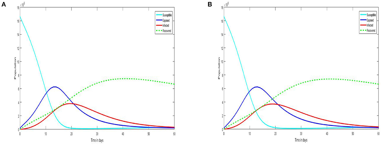
Figure 1. (A) Solution of SEIR model by using Euler method. (B) Solution of SEIR model by using Runge Kutta method.

Figure 1B shows the simulation result of the SEIR COVID-19 outbreak with the effects of partially and fully vaccinated individuals by using the fourth order Runge–Kutta method. Here, the exposed and infected population raises and then approaches near zero. Clearly, from the graph and data, we can predict that during the 20^th day, the rate of infection was going to peak position and then slowly approaches close to zero with respect to time, whereas the susceptible population decreases drastically at first and then slowly move toward stability. In the case of a recovered population, the rate of recovery increases gradually and moves toward the equilibrium values. Furthermore, from both Figures 1A, B, we can say that Figure 1B is more accurate than Figure 1A. This is because the Euler method has first order accuracy and the Runge–Kutta method has fourth order accuracy [15]. So, Figure 1B gives a more accurate result. So, overall from this, we can say that the incorporation of the V_p and V_f parameters into the model has worked well and successfully decreases the spread of COVID-19 in Trivandrum city.

4.2. Absolute value difference of SEIR model solution between the two methods

Figure 2 demonstrates the absolute value difference of the SEIR model between the Euler and the fourth order Runge–Kutta methods. From this, we comment that the absolute value has a sudden raise in the beginning stage. This is due to the increase in the value of the SEIR model solution, which increases the absolute value difference up to the peak and then decreases over time. The difference between both solutions is large in the time interval [3, 16]. Supplementary Table 5 shows the absolute value difference of the solution for the considered 55 days.

FIGURE 2

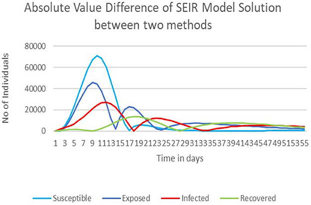
Figure 2. The absolute value difference of SEIR model solution between two methods.

From Supplementary Table 5, the largest absolute value difference of the solutions of S(t), E(t), I(t), and R(t) are 70,931, 45,597, 27,276, and 13,548, respectively, at the time t = 10, 9, 12, and 18. From these data, we conclude that the absolute value difference between the two methods is large.

4.3. Comparison between the Euler and fourth order Runge–Kutta methods

In this subsection, we have introduced the comparison between the Euler and fourth order Runge–Kutta methods. Here, Figures 3A, B, 4A, B demonstrate the comparison between these two methods for the cases of susceptible, exposed, infected, and recovered populations, respectively. The generated values between the two methods show the same behavior with a slight variation and produce similar results. Here, in Figure 3B, initially, the number of exposed individuals increases steeply and then decreases over a period of time. The increase in the exposed population is due to the incorporation of the fact that all partially vaccinated individuals are assumed to be getting exposed to the infection. In addition, in Figure 4A, initially, the number of infected individuals increases steeply over a period of time and decreases eventually. The decrease in infection is due to the increase in recovered individuals. Since those who recovered from the infection are been transferred to the recovered compartment. Furthermore, we assumed the fact that fully vaccinated individuals directly move to the recovered class. Similarly, in Figure 4B, the number of recovered individuals increases slowly and attains a peak on the 35th day. Since the incubation period is 5–14 days, this is one of the reasons for the slowness in the recovered population.

FIGURE 3

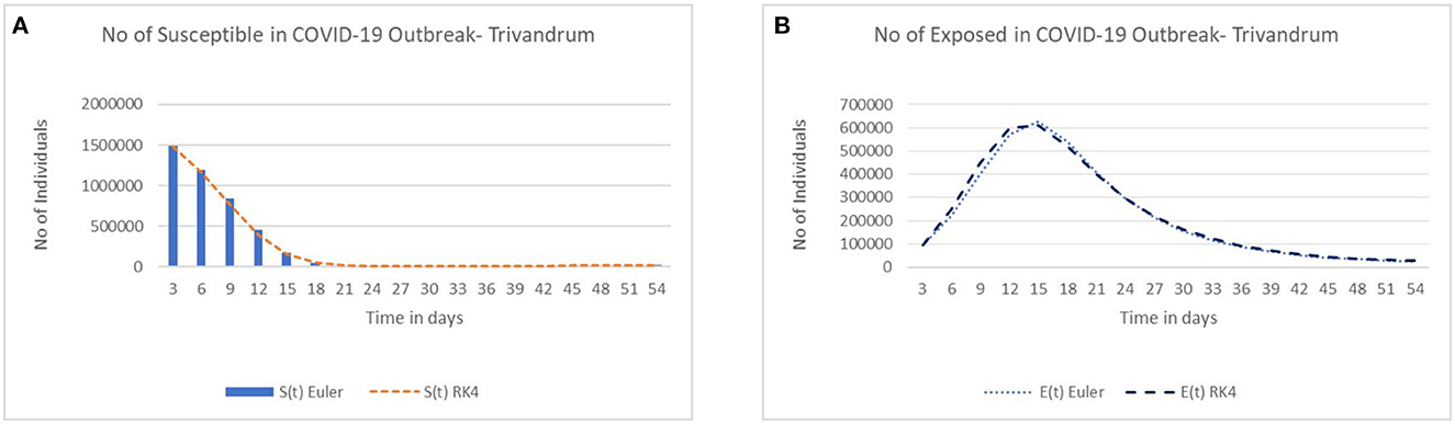
Figure 3. (A) Comparison between Euler and fourth order Runge Kutta method in the case of susceptible population. (B) Comparison between Euler and fourth order Runge Kutta method in the case of exposed population.

FIGURE 4

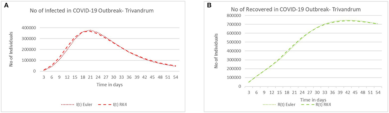
Figure 4. (A) Comparison between Euler and fourth order Runge Kutta method in the case of infected. (B) Comparison between Euler and fourth order Runge Kutta method in the case recovered population.

4.4. Comparing the model with actual data

Using the generated data and actual data from Supplementary Tables 6, 7, we have plotted a graph that compares the model data with the actual data for the infected and recovered populations. Figures 5A, 6A demonstrate that the real data do not coincide or fit well with the generated results of the model. From these displayed figures, we observe that the generated values and the actual values do not match or coincide well. This may be due to the unexpected rise of the infected population in the real world, particularly Trivandrum. Here, the actual data curve remains at the bottom and looks like a straight line. So, to get a clear picture of actual data, we have plotted it separately in Figures 5B, 6B. This shows the daily variation of infected and recovered individuals over a period of 55 days in Trivandrum city.

FIGURE 5

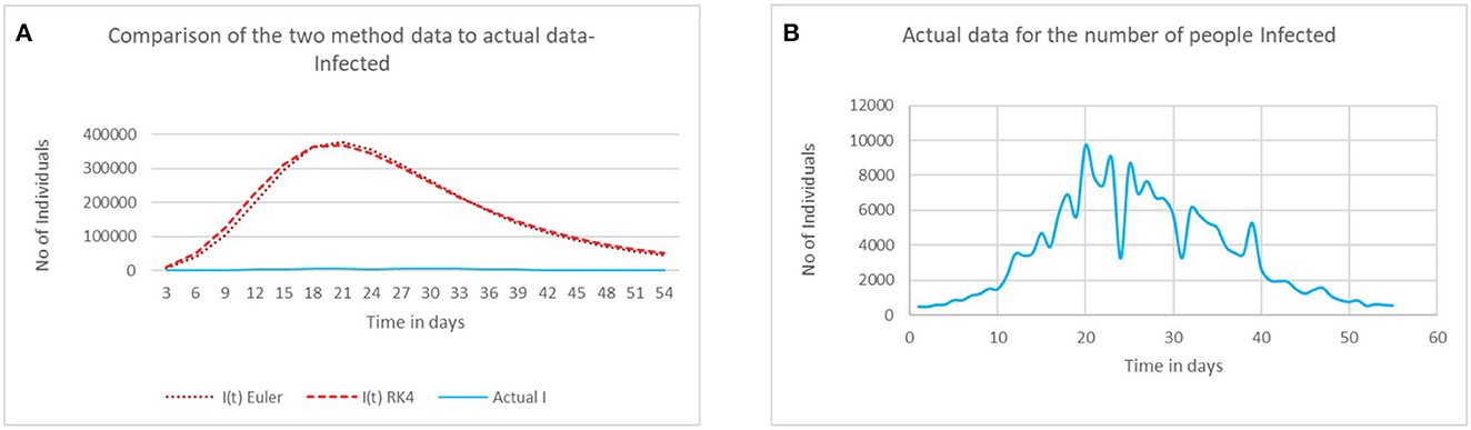
Figure 5. (A) Comparing the model with actual data- infected. (B) Actual data for the number of people infected.

FIGURE 6

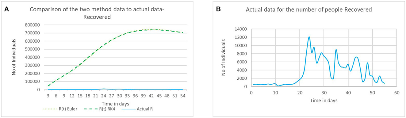
Figure 6. (A) Comparing the model with actual data- recovered. (B) Actual data for the number of people recovered.

4.5. Curve fitting with actual data

By doing some modifications in the parameter values, we were able to fit the model with our real-world data, which are demonstrated in Figures 7A, B. It shows the comparison of curve-fitted data from 55 days with the real-world data for the infected and recovered populations. Furthermore, Supplementary Table 8 shows the comparison of data of the fitted model to the real-life data for both the infected and recovered populations. Hence, from this, we were able to match the generated values with real-world data.

FIGURE 7

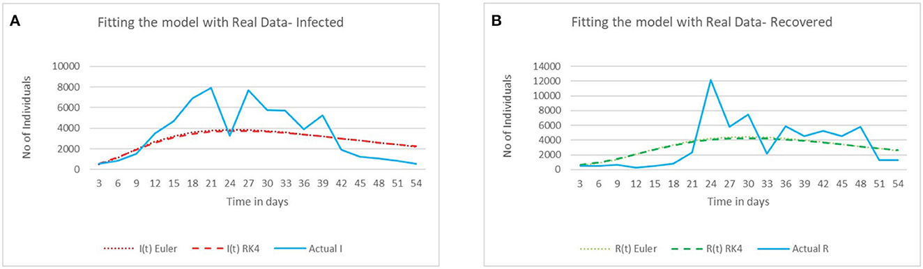
Figure 7. (A) Curve fitting with actual data for infected population. (B) Curve fitting with actual data for recovered population.

5. Conclusion

The solution to the SEIR model with the effects of partially and fully vaccinated individuals are discussed in this study. Here, we solve our model by using the Euler and fourth order Runge–Kutta methods for the capital of Kerala, Trivandrum city. Using MATLAB, we have generated the values and graphs for 55 days from 1 January 2022 to 24 February 2022. The simulation result shows that both methods have the same behavior and produce similar results for all the population groups. Furthermore, we found that the fourth order Runge–Kutta method is more accurate than the Euler method. The absolute value difference between these two methods is obtained. This shows that the differences of the solution between these two methods are large at the time interval [3, 16]. Then, we have compared the infected and recovered data of the two methods with actual data, which is described in Figures 5A, 6A. We observed that the graph does not match with the actual data due to a huge rise in the infected and recovered populations and also overestimation of parameters such as γ and δ. Meanwhile fully vaccinated population plays a vital role in our model. It triggers the recovery rate. Eventually some studies and new articles [17] show that COVID-19 vaccine remains effective in preventing severe disease, but its effectiveness can wane over time. According to Dr.Rommel Tickoo, boosters are being recommended because data are showing that the protection of vaccine declines over time, particularly those who were vaccinated long before. Furthermore, he added that it is concern about new COVID-19 variant, such as Omicron. He suggests that getting a booster dose can decrease the risk of infection and severe illness from virus. In India, it has been 15 months of completion in vaccination drive. Still, 37% of eligible individuals are not been fully vaccinated yet, whereas in Trivandrum, 32% have been not fully vaccinated. So, this is also one of the reasons of mismatch of generated values with actual data in Figures 5A, 6A. Hence, in future, by doing parameter estimation, we can modify our model and can evaluate the flaws.

Data availability statement

The original contributions presented in the study are included in the article/Supplementary material, further inquiries can be directed to the corresponding author.

Author contributions

AM, GC and QA-M: conception and design of study and revising the manuscript critically for important intellectual content. GC and QA-M: handling the numerical issues. AM and GC: analysis and/or interpretation of data and drafting the manuscript. All authors contributed to the article and approved the submitted version.

Conflict of interest

The authors declare that the research was conducted in the absence of any commercial or financial relationships that could be construed as a potential conflict of interest.

Publisher's note

All claims expressed in this article are solely those of the authors and do not necessarily represent those of their affiliated organizations, or those of the publisher, the editors and the reviewers. Any product that may be evaluated in this article, or claim that may be made by its manufacturer, is not guaranteed or endorsed by the publisher.

Supplementary material

The Supplementary Material for this article can be found online at: https://www.frontiersin.org/articles/10.3389/fams.2023.1124897/full#supplementary-material

Footnotes

1. ^Ministry of Health and Family Welfare (2021). Available online at: https://www.cowin.gov.in (accessed April 08, 2021).

2. ^COVID-19 BHARAT (2021). Available online at: https://www.covid19.bharat.org (accessed April 08, 2021).

References

1. Centers for Disease Control Prevention. CDC in India. (2021). Available online at: https://www.cdc.gov/flu/pandemic.html (accessed April 08, 2021).

2. Eddy F, Jeremy RB, Laurent B, Carolyn SC, Niall DF, Arthur SS, et al. COVID-19 associated acute respiratory distress syndrome: is a different approach to management warranted? Lancet Respir Med. (2020) 8:816–21. doi: 10.1016/S2213-2600(20)30304-0

PubMed Abstract | CrossRef Full Text | Google Scholar

3. Rizky A, Mochammad A, Sri P. Comparison of numerical simulation of epidemiological model between Euler method with 4th order Runge Kutta method. Int J Glob Operat Res. (2021) 2:37–44. doi: 10.47194/ijgor.v2i1.67

CrossRef Full Text | Google Scholar

4. Tareque H, Musa M, Babul H. Numerical study of Kermack-Mckendrik SIR model to predict the outbreak of Ebola virus diseases using Euler and fourth order Runge-Kutta methods. Am Sci Res J Eng Technol Sci. (2017) 37:1–21.

Google Scholar

5. Gunasundari C, Senthilkumaran M. Stability analysis of delayed predator prey model with disease in prey. Int J Comput Appl. Math. (2017) 12:509–39. doi: 10.1016/j.apm.2016.10.003

CrossRef Full Text | Google Scholar

6. Haneen B, Nabil S, Omar AA. Fractional conformable stochastic integrodifferential equations: existence, uniqueness, and numerical simulations utilizing the shifted legendre spectral collocation algorithm. Math Probl Eng. (2022) 2022:21. doi: 10.1155/2022/5104350

CrossRef Full Text | Google Scholar

7. Banan M, Omar AA, Salam A, Hamed A. Numerical solutions and geometric attractors of a fractional model of the cancer-immune based on the Atangana-Baleanu-Caputo derivative and the reproducing kernel scheme. Chin J Phys. (2022) 80:463–83. doi: 10.1016/j.cjph.2022.10.002

CrossRef Full Text | Google Scholar

8. Omar AA, Hamed A, Mohammed A. Numerical Hilbert space solution of fractional Sobolev equation in (1+1)-dimensional space. Math Sci. (2022) 2022. doi: 10.1007/s40096-022-00495-9

CrossRef Full Text | Google Scholar

9. Kolokolnikov T, Iron D. Law of mass action and saturation in SIR model with application to Coronavirus modelling. Infect Dis Model. (2021) 6:91–7. doi: 10.1016/j.idm.2020.11.002

PubMed Abstract | CrossRef Full Text | Google Scholar

10. Xu F, Connell M, Cressman R. Spatial spread of an epidemic through public transportation systems with a hub. Math Biosci. (2013) 246:164–75. doi: 10.1016/j.mbs.2013.08.014

PubMed Abstract | CrossRef Full Text | Google Scholar

11. Peng L, Yang W, Zhang D, Zhuge C, Hong L. Epidemic analysis of COVID-19 in China by dynamical modeling. MedRxiv. (2013) doi: 10.1101/2020.02.16.20023465

PubMed Abstract | CrossRef Full Text | Google Scholar

12. Hurit RU, Mungkasi S. The Euler, Heun, and fourth order Runge-Kutta solutions to SEIR model for the spread of meningitis disease. J Mat Pendidikan Mat. (2021) 6:140–153. doi: 10.31943/mathline.v6i2.176

CrossRef Full Text | Google Scholar

13. Alsakaji HJ, Rihan FA, Hashish A. Dynamics of a stochastic epidemic model with vaccination and multiple time-delays for COVID-19 in the UAE. Hindawi Compl. (2022) 2022:15. doi: 10.1155/2022/4247800

CrossRef Full Text | Google Scholar

14. Kandasamy P, Thilagavathy K, Gunavathi K. Numerical Methods. S Chand and Company Limited (1997).

15. Butcher JC. Numerical Methods for Ordinary Differential Equation. New York, NY: John Wiley and Sons Inc. (2003).

PubMed Abstract | Google Scholar

16. Population Census. (2011). Available online at: https://www.census2011.co.in (accessed April 08, 2021).

17. Booster-dose-of-covid-19-vaccine-begins-today. (2021). Available online at: https://www.ndtv.com/health/booster-dose-of-covid-19-vaccine-begins-today-why-you-must-take-it-2699353/amp/1 (accessed April 08, 2021).

Keywords: COVID-19, mathematical model, Euler method, Runge Kutta method, Trivandrum, numerical simulation

Citation: M A, C G and Al-Mdallal QM (2023) Mathematical modeling and simulation of SEIR model for COVID-19 outbreak: A case study of Trivandrum. Front. Appl. Math. Stat. 9:1124897. doi: 10.3389/fams.2023.1124897

Received: 15 December 2022; Accepted: 20 January 2023;
Published: 15 February 2023.

Edited by:

Youssri Hassan Youssri, Cairo University, Egypt

Reviewed by:

Omar Abu Arqub, Al-Balqa Applied University, Jordan
Ahmed Atta, Ain Shams University, Egypt

Copyright © 2023 M, C and Al-Mdallal. This is an open-access article distributed under the terms of the Creative Commons Attribution License (CC BY). The use, distribution or reproduction in other forums is permitted, provided the original author(s) and the copyright owner(s) are credited and that the original publication in this journal is cited, in accordance with accepted academic practice. No use, distribution or reproduction is permitted which does not comply with these terms.

*Correspondence: Qasem M. Al-Mdallal, yes q.almdallal@uaeu.ac.ae

ORIGINAL RESEARCH article

Mathematical modeling and simulation of SEIR model for COVID-19 outbreak: A case study of Trivandrum

1. Introduction

2. Methodology

2.1. Formulation of the SEIR model

2.2. Transformation of Euler equations for our SEIR model

2.3. Transformation of Runge–Kutta equations for our SEIR model

2.4. General algorithm for the Euler and Runge–Kutta methods

3. Applications

3.1. Solution obtained by using the Euler method

3.2. Solution obtained by using the fourth order Runge–Kutta method

4. Results and discussion

4.1. Simulation result of the Euler and Runge–Kutta methods

4.2. Absolute value difference of SEIR model solution between the two methods

4.3. Comparison between the Euler and fourth order Runge–Kutta methods

4.4. Comparing the model with actual data

4.5. Curve fitting with actual data

5. Conclusion

Data availability statement

Author contributions

Conflict of interest

Publisher's note

Supplementary material

Footnotes

References

People also looked at