The evolution of resource distribution, slow diffusion, and dispersal strategies in heterogeneous populations

1. Introduction

The study of spatial effects in a heterogeneous environment for two competing or cooperating species provides a vital tool for use in population ecology that is well-suited to capturing real-world phenomena for geographies with different attributes. The reaction-diffusion equations [1–6] are typically and widely used as a model of spatial effect incorporating parameters such as local growth rate, dispersal rate, and carrying capacity, which may vary over time and space. These reaction-diffusion equations have been improved continuously to enhance their ability to explain real-world situations. In practice, many biological events show that population density and the dynamics of population behaviors are greatly affected by the reaction and diffusion terms of the model. For population dispersion, not only is the diffusion speed relevant, but the strategy by which species diffuse in nature is also a vital issue that has recently become a critically important element of in-depth analysis. In the implementation of diffusion models, numerous dispersal strategies have appeared in models using biological particles; these strategies should be specified for species' improved survival. In a model with regular diffusion terms, when resources are distributed unequally or in the case of a non-constant carrying capacity, a non-feasible system may appear when very high levels of migration are observed from a location with higher per-capita available resources to a less fruitful region. Moreover, the ideal free distribution has been approximated in [7] for a spatially dispersed population. This exhibits a property of diffusion toward the direction of improved fitness to produce a stable equilibrium that can be expected to represent a solution in a temporally fixed but spatially heterogeneous environment. However, any individual deviation from the ideal population distribution will reduce the fitness of the species. The fitness pattern is presented in Figure 1.

FIGURE 1

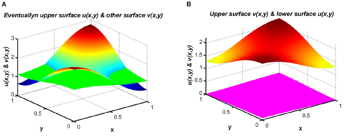
Figure 1. Population densities under (2.1) for (A) coexistence signature, and (B) extinction vs. survival.

The concepts of different diffusion strategies, predator–prey systems, nutrient–phytoplankton systems with toxic effects on phytoplankton, and pest control are often closely connected to the creation and diffusion of knowledge and the technological evolution of society. For more advanced work on the dynamics of species management, see [8, 9]. Additionally, in most scenarios, resources are not unlimited and environmental conditions are not optimal. Population growth may be resisted by environmental resources due to issues like food, climate, water availability, and others. Naturally, species tend to move toward superior locations in terms of food, safety, or any other survival instinct. Thus, they do not simply diffuse randomly; instead, they choose to migrate to attain a better existence. Along with the aforementioned observation, Braverman and Braverman [10] were the first to introduce the notion of carrying-capacity–driven diffusion, inspired by the selection of optimal harvesting strategies, which have major biological significance. The stability properties of the model were first studied in [11] with logistic-type growth. In this type of diffusion strategy, the diffusive transport of the population is considered proportional to the gradient of population density per unit capacity instead of simply the population density. The advantage of the carrying-capacity–driven diffusion strategy relative to classical diffusion in terms of completion was initially delineated in [12] considering logistic growth, and further explored in [13] for a wide variety of growth functions. The latest modification to species migration strategy was first introduced in 2016 by Braverman and Kamrujjaman in [14, 15] and is known as the resource-based diffusion strategy. Under this type of diffusion strategy, species diffuse according to their respective resource-based dispersal function, in which the diffusive movement of species is considered proportional to the gradient of population density per unit resource rather than simply to carrying capacity. Compared to random diffusion, the main advantage of using this type of diffusion is that its solution coincides with the ideal free distribution under certain conditions with respect to carrying capacity and resource function. In this context, we can mention several fields studied on the basis of a single species: for example, studies of grazing animal populations [16], invasive weeds or plants like Solanum carolinense in Europe [17], or North American Prairie duck [18]; these studies were conducted in the experimental field, and the experimental results show that the dispersion of these species is directed toward the area of higher per-capita available resources. Similar observations will be noted when considering a pair of species in a heterogeneous environment.

It is most significant for the dynamics of two competing populations to examine how the density of one organism or species changes relative to others in space and time to survive under this competitive scenario. In a competition, the main possible outcomes are that both species triumph or one survives as the other goes extinct. Additionally, in ecology, operating under some instinct, both species may leave the area in a competition that yields neither extinction nor coexistence. For a historical discussion of the proposed models, readers are referred to [2, 7, 12, 13, 15, 19–22]. It should also be mentioned that lower diffusion rates were favored by [2] in a heterogeneous environment, since the authors found that the fitness levels of species differ only according to their dispersal rate, and population growth falls as the diffusion coefficient increases. Accordingly, in our study, the results of [2] have been extended to a scenario where the strategy of dispersion is the same for both species, rather than random, which is dissimilar from [11]. This paper focuses on estimating the possible benefits to a species adopting a strategy based on the availability of resources, in contrast with the well-established study of other diffusion strategies. We also examine the significance of higher diffusion and intrinsic growth rates in a heterogeneous environment for two competing species. These are the central facets of our interest in studying a pair of species with various resource distributions. See additionally [23], where a single-species population was studied by considering Gilpin-Ayla growth and harvesting; this study was mostly concerned with diffusion strategy, migration coefficient, and harvesting. The present, in contrast, study explores population distribution under an approach that has many applications in various areas of ecology and economics; readily applicable examples are applications in river and ocean ecology relating to observations of the seasonal behaviors of various species, including wild animals and winter birds. Three critical issues are primarily considered: (i) diffusion strategies for scenarios in which the competing species have equal and unequal carrying capacities; (ii) slow dispersal effects; and (iii) resource distributions, with corresponding demonstrations for each issue. Additionally, we demonstrate that there are certain evolutionary advantages of employing a carrying-capacity- and resource-based diffusion strategy despite classical diffusion.

The main findings of the present study are as follows:

1. We study the global existence of solutions to the competition model by considering two main ecological settings: Case I, in which the carrying capacities of the interacting species are unequal, and Case II, in which carrying capacity is equal with different diffusion strategies. We find effects of diffusion speed as well as interactions between resources and capacity function.

2. For unequal carrying capacity, if the first species follows a carrying-capacity–driven diffusion strategy while the other adopts resource-based diffusion, then the first species always survives in competition in cases of an equal intrinsic growth rate. We also observe that more resource consumption by the species with the greater carrying capacity will drive the one with the lower capacity to extinction in the competition.

3. When both species adopt the same resource-based diffusion strategy, the species that consumes more, with a higher carrying capacity ratio, is guaranteed to survive in the competition.

4. In addition, in cases of the same diffusion strategy, a species that diffuses slowly has an evolutionary advantage compared to others; this extends the result of [2] to resource-based diffusion. We find that a higher diffusion coefficient is unconducive to sustained competition.

5. In cases of species with different proportions of carrying capacity and intrinsic growth rates, coexistence is also evident. In this situation, the species' elevated growth rate is noted, incorporating a higher proportion of the available resources in competition.

6. When the carrying capacity of both species is equal, we study the case of competitive exclusion as an abbreviation of carrying capacity and one of the resource functions for which the globally stable semi-trivial equilibrium is observed to obtain.

7. We also present some numerical results for both one- and two-dimensional cases. As we know, the theory does not give any idea of the shape of the non-zero equilibrium profiles, which we explore numerically.

8. We show via numerical computation that the existence of a state of coexistence is also possible due to the influence of migration coefficients. Intrinsic growth rates can also play an important role in sustaining both species in competition.

9. Furthermore, for the case of time-periodic parameters, numerical results suggest the existence of a time-periodic state with the same period.

The manuscript is organized as follows. A description of the mathematical model is provided in Section 2. Section 3 describes the results of the model in terms of the existence and uniqueness of solutions for non-negative and non-trivial initial conditions; these results also justify the positivity of the solution. A coexistence analysis and quasi-trivial equilibrium with some preliminary results for the case of unequal carrying capacity that are applicable in the remainder of the discussion are presented in Section 4. Moreover, Section 4 also presents the main results and proof of the study: the global existence of an equilibrium for competitive exclusion and coexistence analysis for K_u ≢ K_v. Section 5 considers the competitive exclusion of population for the case of K_u ≡ K_v with some auxiliary results. Section 6 presents a numerical simulation and illustrates the application of this study for ecological implementations. The numerical computation for the case of two spatial dimensions is presented in Section 6.1 in the form of contour plots for both space- and time-dependent functions. This is highly novel to our study; it captures the ecological impact of this study in a more biologically feasible way and justifies the theoretical underpinnings of the main result through numerical assertion. Finally, Section 7 provides a summary and discussion of the model presented in this study.

2. Mathematical model

In our model, we consider the two species [notionally, u(t, x) and v(t, x)] as a competitive system, isolated and spatially distributed in a heterogeneous environment. Here, u(t, x) and v(t, x) represent the population densities of two striving species, each undergoing diffusion under similar resource-based diffusion strategies while the most troubling situation for them is when they fight for the same fundamental resources. The dispersal strategies of the species are also considered to stipulate two positive distribution functions with different carrying capacity proportions; i.e., the system considers the carrying capacities of the competing species to be dissimilar, with no-flux/zero Neumann boundary conditions contemplated through the domain boundary. The use of homogeneous Neumann boundary conditions represents a scenario in which (i) the populations are isolated in a closed area and there is no movement across the boundaries of this area, and (ii) spatial immigration is compensated through emigration to the domain. Under these assumptions, the corresponding competitive model with homogeneous Neumann boundary conditions associated with positive and non-trivial initial conditions is defined as follows:

$\begin{array}{ll}\{\begin{array}{l}\frac{\partial u}{\partial t}=d_1\Delta \left(\frac{u\left(t,x\right)}{M\left(x\right)}\right)+r_1\left(x\right)u\left(t,x\right)\left(1-\frac{u+v}{K_u\left(x\right)}\right),t>0,x\in \omega ,\\ \frac{\partial v}{\partial t}=d_2\Delta \left(\frac{v\left(t,x\right)}{N\left(x\right)}\right)+r_2\left(x\right)v\left(t,x\right)\left(1-\frac{v+u}{K_v\left(x\right)}\right),t>0,x\in \omega ,\\ \text{n}·\nabla \left(\frac{u\left(t,x\right)}{M\left(x\right)}\right)=\text{n}·\nabla \left(\frac{v\left(t,x\right)}{N\left(x\right)}\right)=0,x\in \partial \omega ,\\ u_0\left(x\right)=u\left(0,x\right),v_0\left(x\right)=v\left(0,x\right),x\in \omega .\end{array}& (2.1)\end{array}$

We assume that K_u > 0, K_v > 0; these expressions represent the carrying capacity of the environment for the corresponding species, where r_i > 0, i = 1, 2 are the intrinsic growth rates, and M, N are the species resource functions. All fall within the class of $C^{1+\alpha }(\overline{\omega })$, where ω is an open non-empty isolated bounded domain in ℝⁿ with ∂ω ∈ C^2+α, and 0 < α < 1 for any x ∈ ω, which means that r₁(x), r₂(x), K_u(x), K_v(x), M(x), and N(x) are all positive in an open non-empty sub-domain of ω. Here, d₁ > 0 and d₂ > 0 are the migration rates that describe the corresponding dispersal rates of each species. The range of the solutions to (2.1) corresponds to the set p₁ × p₁, which is determined by the corresponding upper and lower solutions.

Suppose u^* and v^* are the stationary solutions of the first and second equation corresponding to (2.1) when only one species survives, so that the semi-trivial equilibria (u^*, 0) and (0, v^*) satisfy

$\begin{array}{r}{d}_1\Delta \left(\frac{u^{*}\left(x\right)}{M\left(x\right)}\right)+r_1\left(x\right)u^{*}\left(1-\frac{u^{*}}{K_u\left(x\right)}\right)=0,\\ x\in \omega ,\text{n}·\nabla \left(\frac{u^{*}}{M}\right)=0,x\in \partial \omega ;& (2.2)\end{array}$

$\begin{array}{r}{d}_2\Delta \left(\frac{v^{*}\left(x\right)}{N\left(x\right)}\right)+r_2\left(x\right)v^{*}\left(1-\frac{v^{*}}{K_v\left(x\right)}\right)=0,\\ x\in \omega ,\text{n}·\nabla \left(\frac{v^{*}}{N}\right)=0,x\in \partial \omega .& (2.3)\end{array}$

Model (2.1) is a specimen of a monotone dynamical system [5, 24, 25]. That is, when the zero equilibrium is not stable, no coexistence equilibrium occurs for the system (2.1), and one of the semi-trivial equilibria is also unstable, the remaining semi-trivial equilibrium solution will be globally asymptotically stable; on the other hand, if both semi-trivial equilibria are unstable, then (2.1) possesses at least one stable coexistence equilibrium.

Resource-based competition model (2.1), with unequal carrying capacities and intrinsic growth rates, is a prevalent ecological model for inter-specific competition that captures the reality observed in nature. Many organisms follow our stated types of diffusion strategy, such as grazing animals [16], marine organisms [26], zooplankton-like protozoa, and wild birds (owls, sparrows, etc., and all kinds of winter birds).

For further analysis, it is also convenient to substitute $w=\frac{u(t,x)}{M(x)}$ and $z=\frac{v(t,x)}{N(x)}$, respectively. Then, system (2.1) is reduced to

$\begin{array}{ll}\{\begin{array}{l}\frac{\partial w\left(t,x\right)}{\partial t}=\left(\frac{d_1}{M\left(x\right)}\right)\Delta w+r_1\left(x\right)w\left(1-\frac{M}{K_u}w-\frac{N}{K_u}z\right),\\ t>0,x\in \omega ,\\ \frac{\partial z\left(t,x\right)}{\partial t}=\left(\frac{d_2}{N\left(x\right)}\right)\Delta z+r_2\left(x\right)z\left(1-\frac{M}{K_v}w-\frac{N}{K_v}z\right),\\ t>0,x\in \omega ,\\ \text{n}·\nabla w=\text{n}·\nabla z=0,x\in \partial \omega ,\\ w_0\left(x\right)=w\left(0,x\right),z_0\left(x\right)=z\left(0,x\right),x\in \omega .\end{array}& (2.4)\end{array}$

The model then reduces to a couple of equations with classical diffusion through smooth and positive space-dependent coefficients $\frac{d_1}{M(x)}$ and $\frac{d_2}{N(x)}$. Next, we analyze the existence, uniqueness, and positivity of solutions to the system (2.4). To do this, we initially confine our observations to a model that represents the action of the system for a single species and for a pair of species.

3. Existence, uniqueness, and positivity of solution

Consider the following directed diffusion model with homogeneous Neumann boundary and positive initial conditions:

$\begin{array}{ll}\{\begin{array}{l}\frac{\partial u}{\partial t}=d_1\Delta \left(\frac{u\left(t,x\right)}{M\left(x\right)}\right)+r_1\left(x\right)u\left(1-\frac{u}{K_u\left(x\right)}\right),t>0,x\in \omega ,\\ \text{n}·\nabla \left(\frac{u}{M}\right)=0,x\in \partial \omega ,u_0\left(x\right)=u\left(0,x\right),x\in \omega .\end{array}& (3.1)\end{array}$

Existence and uniqueness results for species u in the form of the Equation (3.1) are well-established for K_u = M in [13, 20, 27], indicating that the system (3.1) has a unique and stable positive solution. According to [5, 13, 20, 24, 27] the proof of the following Lemma can proceed in the same way as far as M ≡ K_u or M ≢ K_u.

Lemma 1. [20, 27] For any u₀(x) ≥ 0 in ω and u₀(x) ≢ 0 in some open and bounded sub-domain ω_l ⊂ ω, there is a unique solution u(t, x) of model (3.1) and it is positive. If $\frac{M(x)}{K_u(x)}\equiv Constant$, then $u^{*}(x)=K_u(x)$ is the only solution of (3.1), and as t → ∞ the solution converges to K_u(x), otherwise u^*(x) is different from K_u(x).

Similarly, we can construct the existence and uniqueness result for the species v.

The system (2.1) is an example of a monotone dynamical system [15, 28, 29]. According to [1, 13, 15], the system has a unique and positive solution for K_u = K_v = K. The same procedure can be applied to (2.1), which affords the existence and uniqueness of a solution for a coupled system of the Equation (2.1).

Theorem 1. [13] Let u₀(x) and v₀(x) be non-negative on ω. Then for any u₀(x), v₀(x) ∈ C(ω), the system (2.1) has a unique solution (u, v). Furthermore, if (u₀(x), v₀(x)) is non-trivial and non-negative, then for any T > 0, both u(t, x) > 0 and v(t, x) > 0.

In the next section, we express the result based upon the stability of all steady-state solutions of the model (2.1), which are two semi-trivial equilibria (u^*, 0) and (0, v^*), in which only a single species persists, as well as a coexistence state (u^*, v^*), in which both species coexist in the same environment, and finally the trivial equilibrium (0, 0), in which both species leave the area due to competition. The stated results are for the monotone dynamical system that originated in [5]; for the system (2.1), we use a modification in the form previously described in [20] [see [20], Theorem 09, pp. 73 for more details], since system (2.1) follows a monotone dynamical system. Additionally, a few preliminary consequences for the existence of an equilibrium are presented in Section 4.

4. Steady state and global analysis: case I, K_u ≢ K_v

For further analysis of system (2.1), we have extended the following three auxiliary results (to be applied in completing the following discussion), which are already established in [12–15], for K_u = K_v = K.

Lemma 2. [13–15] Suppose M(x), N(x), K_u(x) ≢ K_v(x) are non-constant and r₁(x) ≡ r₂(x) ≡ r(x). If $\frac{M}{K_u}\equiv Constant$, while $\frac{N}{K_u}\not\equiv Constant$ and $\frac{N}{K_v}\not\equiv Constant$ or K_u > K_v in a non-empty open domain x ∈ ω, then a unique and positive stationary solution (0, v^*) to (2.1) occurs, so that

$\begin{array}{ll}{\displaystyle \underset{\omega }{\int }}r\left(x\right)K_u\left(1-\frac{v^{*}}{K_u}\right)dx>0.& (4.1)\end{array}$

Lemma 3. [13–15] Assume that (u_c, v_c) is a positive steady state solution of system (2.1), and K_u > K_v, so that u_c + v_c ≢ K_u; then

${\displaystyle \underset{\omega }{\int }}r\left(x\right)K_u\left(x\right)\left(1-\frac{u_c+v_c}{K_u}\right)dx>0.$

Lemma 4. The zero equilibrium (0, 0) of the model (2.1) is unstable and repelling.

The proof is available in [12, 13], so we have omitted it here.

Next, we examine our key results for the system 2.1 by inspecting the stability of two semi-trivial or quasi-trivial equilibria, namely (u^*, 0) and (0, v^*), that occur when a single species endures alone, as well as a coexistence equilibrium (u^*, v^*), which is a neither quasi-trivial nor trivial equilibrium that satisfies u^*(x) > 0, v^*(x) > 0. If M(x) = K_u(x) and N(x) = K_v(x), then the semi-trivial equilibria will converge to (K_u, 0), and (0, K_v). However, we also confirm that, in this case, the species that survives in the competition will always be the one adopting a carrying-capacity–driven diffusion strategy. After considering all these possibilities, we prove our main results.

Lemma 5. Assume that the functions M(x), N(x), K_u(x), K_v(x) are non-constant and r₁(x) ≡ r₂(x) ≡ r(x). If K_u ≥ K_v for all x ∈ ω, and $\frac{M}{K_u}\equiv Constant$ while $\frac{N}{K_u}\not\equiv Constant$ or $\frac{N}{K_v}\not\equiv Constant$ or K_u(x) > K_v(x) in a non-empty, bounded, and open domain ω, then no coexistence state (u_c, v_c) of the system (2.1) will exist.

Proof. We are now interested only in cases where K_u(x) > K_v(x), because the result for K_u(x) ≡ K_v(x) was already established in [13] for all x ∈ ω_l ⊆ ω. First, let us speculate to the contrary that there prevails a strictly positive equilibrium state (u_c, v_c) of (2.1), and we will prove that this assumption leads to a contradiction. Under this assumption, the solution (u_c, v_c) satisfies

$\begin{array}{ll}\{\begin{array}{l}{d}_1\Delta \left(\frac{u_c\left(x\right)}{M\left(x\right)}\right)+r\left(x\right)u_c\left(1-\frac{u_c\left(x\right)+v_c\left(x\right)}{K_u\left(x\right)}\right)=0,x\in \omega ,\\ \text{n}·\nabla \left(\frac{u_c}{M}\right)=0,x\in \partial \omega .\\ d_2\Delta \left(\frac{v_c\left(x\right)}{N\left(x\right)}\right)+r\left(x\right)v_c\left(1-\frac{u_c\left(x\right)+v_c\left(x\right)}{K_v\left(x\right)}\right)=0,x\in \omega ,\\ \text{n}·\nabla \left(\frac{v_c}{N}\right)=0,x\in \partial \omega .\end{array}& (4.2)\end{array}$

Adding the first two equations in (4.2), integrating over ω, and applying the Neumann boundary conditions, we obtain:

$\begin{array}{ll}{\displaystyle \underset{\omega }{\int }}r\left(x\right)u_c\left(1-\frac{u_c+v_c}{K_u}\right)dx+{\displaystyle \underset{\omega }{\int }}r\left(x\right)v_c\left(1-\frac{u_c+v_c}{K_v}\right)dx=0.& (4.3)\end{array}$

Since K_u > K_v, it follows that $\left(1-\frac{u_c+v_c}{K_v}\right)<\left(1-\frac{u_c+v_c}{K_u}\right)$. Thus, (4.3) implies:

$\begin{array}{ll}{\displaystyle \underset{\omega }{\int }}r\left(x\right)\left(u_c\left(x\right)+v_c\left(x\right)\right)\left(1-\frac{u_c+v_c}{K_u}\right)dx>0.& (4.4)\end{array}$

Now, $\left(u_c+v_c\right)\left(1-\frac{u_c+v_c}{K_u}\right)=K_u\left(1-\frac{u_c+v_c}{K_u}\right)+\left(u_c+v_c-K_u\right)\left(1-\frac{u_c+v_c}{K_u}\right).$

Multiplying by r(x) and integrating the above inequality over ω gives:

$\begin{array}{l}{\displaystyle \underset{\omega }{\int }}r\left(x\right)K_u\left(1-\frac{u_c+v_c}{K_u}\right)dx>{\displaystyle \underset{\omega }{\int }}r\left(x\right)\frac{{\left(u_c+v_c-K_u\right)}^2}{K_u}dx>0\end{array}$

Therefore,

$\begin{array}{ll}{\displaystyle \underset{\omega }{\int }}r\left(x\right)K_u\left(1-\frac{u_c+v_c}{K_u}\right)dx>0,& (4.5)\end{array}$

which is only valid if u_c + v_c ≢ K_u(x). Hence, we need to consider the above two cases for K_u(x) > K_v(x).

Case 1: When u_c + v_c ≡ K_u(x), $w_c=\frac{u_c}{M}$ satisfies Δw_c = 0, x ∈ ω, ∇w_c = 0; and therefore, by the Maximum Principle [30], we have w_c ≡ Constant.

This implies that $\frac{u_c}{M}\equiv Constant$, so u_c ≡ c_mK_u such that v_c = K_u − c_mK_u = (1 − c_m)K_u, which is constant only when c_m = 1, since K_u(x) is variable.

Case 2: Thus, we have to impose only one condition when u_c + v_c ≢ K_u(x) or K_u > K_v in some non-empty open domain. Examine the following eigenvalue problem:

$\begin{array}{r}{d}_1\Delta \left(\frac{\varphi }{M}\right)+r\left(x\right)\varphi \left(1-\frac{u_c+v_c}{K_u}\right)=\sigma \varphi ,x\in \omega ,\\ \text{n}·\nabla \left(\frac{\varphi }{M}\right)=0,x\in \partial \omega .\end{array}$

Following from the fact of variational characterization of eigenvalues [[5], Theorem 2.1], its principal eigenvalue is conferred by

$\begin{array}{l}{\sigma }_1={\displaystyle \underset{\varphi \ne 0,\varphi \in W^{1,2}}{sup}}\\ \frac{{\displaystyle \underset{\omega }{\int }}-d_1|\nabla \left(\frac{\varphi }{M}\right){|}^{2}dx+{\displaystyle \underset{\omega }{\int }}r\left(x\right)\left(\frac{{\varphi }^2}{M\left(x\right)}\right)\left(1-\frac{u_c+v_c}{K_u}\right)dx}{{\displaystyle \underset{\omega }{\int }}\left(\frac{{\varphi }^2}{M\left(x\right)}\right)dx}.& (4.6)\end{array}$

Upon substituting ϕ = M(x), and using (4.5), we obtain:

$\begin{array}{l}{\sigma }_1\ge \frac{{\displaystyle \underset{\omega }{\int }}r\left(x\right)K_u\left(1-\frac{u_c+v_c}{K_u}\right)dx}{{\displaystyle \underset{\omega }{\int }}{K}_u\left(x\right)dx}>0.\end{array}$

However, (w_c, z_c) is a steady state solution of (2.1); w_s satisfies

$\begin{array}{r}{d}_1\Delta w_c+r\left(x\right)w_c{K}_u\left(x\right)\left(1-\frac{M}{K_u}{w}_c-\frac{N}{K_u}{z}_c\right)=0,x\in \omega ,\\ \nabla w_c=0,x\in \partial \omega .\end{array}$

and is therefore a positive principal eigenfunction of (4.6) along with principal eigenvalue 0. This contradicts σ₁ > 0, which concludes the proof.□

Lemma 6. Suppose the functions M(x), N(x), K_u(x), K_v(x) are non-constant and r₁(x) ≡ r₂(x) ≡ r(x). If K_u ≥ K_v for all x ∈ ω, and $\frac{M}{K_u}\equiv Constant$ while $\frac{N}{K_u}\not\equiv Constant$ or $\frac{N}{K_v}\not\equiv Constant$ or K_u(x) > K_v(x) in a non-empty, bounded, and open domain ω, then (0, v^*) is unstable for the system (2.1).

Proof. Taking the linearization of (2.1) over (0, v^*) for the case K_u > K_v, we obtain:

$\begin{array}{l}\begin{array}{l}\frac{\partial u}{\partial t}=d_1\Delta \left(\frac{u}{M}\right)+r\left(x\right)u\left(1-\frac{v^{*}}{K_u}\right),t>0,x\in \omega ,\\ \frac{\partial v}{\partial t}=d_2\Delta \left(\frac{v}{N}\right)+r\left(x\right)v\left(1-\frac{2v^{*}}{K_v}\right)-r{v}^{*}\frac{u\left(t,x\right)}{K_u\left(x\right)},t>0,x\in \omega ;\end{array}\end{array}$

and studying the associative eigenvalue problem of the equation u,

$\begin{array}{r}{d}_1\Delta \left(\frac{\varphi }{M}\right)+r\left(x\right)\varphi \left(1-\frac{v^{*}}{K_u}\right)=\sigma \varphi ,x\in \omega ,\\ \text{n}·\nabla \left(\frac{\varphi }{M}\right)=0,x\in \partial \omega .& (4.7)\end{array}$

The quasi-trivial equilibrium (0, v^*) will not be stable if the principal eigenvalue is positive. Next, considering (4.7): according to [5] (Theorem 2.1), the principal eigenvalue is stated by

$\begin{array}{l}{\sigma }_1={\displaystyle \underset{\varphi \ne 0,\varphi \in W^{1,2}}{sup}}\frac{{\displaystyle \underset{\omega }{\int }}-d_1|\nabla \left(\frac{\varphi }{M}\right){|}^{2}dx+{\displaystyle \underset{\omega }{\int }}r\left(x\right)\left(\frac{{\varphi }^2}{M\left(x\right)}\right)\left(1-\frac{v^{*}}{K_u}\right)dx}{{\displaystyle \underset{\omega }{\int }}\left(\frac{{\varphi }^2}{M\left(x\right)}\right)dx}.\end{array}$

upon substituting ϕ = M(x) and using (4.1) from Lemma 2 for K_u > K_v we obtain:

$\begin{array}{l}{\sigma }_1\ge \frac{{\displaystyle \underset{\omega }{\int }}r\left(x\right)K_u\left(1-\frac{v^{*}}{K_u}\right)dx}{{\displaystyle \underset{\omega }{\int }}{K}_{u}dx}>0.\end{array}$

Thus, σ₁ > 0, which concludes the proof.□

Theorem 2. Suppose the functions M(x), N(x), K_u(x), K_v(x) are non-constant and r₁(x) ≡ r₂(x) ≡ r(x). If K_u ≥ K_v for all x ∈ ω, and $\frac{M}{K_u}\equiv Constant$ while $\frac{N}{K_u}\not\equiv Constant$ or $\frac{N}{K_v}\not\equiv Constant$ or K_u(x) > K_v(x) in a non-empty, bounded, and open domain ω, then (K_u, 0) of (2.1) is globally asymptotically stable.

Proof. According to Lemma 4, (0, 0) is a repeller. By Lemma 5, no coexistence equilibrium exists for the system (2.1); additionally, by Lemma 6, (0, v^*) is unstable as far as K_u > K_v. Therefore, for a strong monotone dynamical system [15, 28, 29], the other quasi-trivial equilibrium (K_u, 0) is globally asymptotically stable.□

Similarly, under the assumption of Lemma 6 with $\frac{M(x)}{K_u(x)}\not\equiv Constant$ as well as $\frac{M(x)}{K_v(x)}\not\equiv Constant$ while $\frac{N(x)}{K_v(x)}\equiv Constant$, and for K_u < K_v in a non-empty open domain, we can establish that (u^*, 0) is also unstable.

The following remark follows the proof of Theorem 2.

Remark 1. Suppose the functions M(x), N(x), K_u(x), K_v(x) are non-constant and r₁(x) ≡ r₂(x) ≡ r(x). If K_u ≤ K_v for all x ∈ ω, and $\frac{N}{K_v}\equiv Constant$ while $\frac{M}{K_u}\not\equiv Constant$ or $\frac{M}{K_v}\not\equiv Constant$ or K_u(x) < K_v(x) in a non-empty, bounded, and open domain ω, then (0, K_v) of (2.1) is globally asymptotically stable.

Similar results are presented in Appendix A for the case of K_u ≢ K_v, when both resource functions are proportional to their respective carrying capacity. At this point, we have identified the global existence of competitive exclusion, considering cases of unequal carrying capacity while other parameters are fixed.

Remark 2. Suppose the functions M, K_u, K_v are constant and r₁ ≡ r₂ ≡ r, d₁ ≡ d₂ ≡ d, while $\frac{M}{K_u}\equiv Constant$ and $\frac{N(x)}{K_v}\not\equiv Constant$. Then, for K_u > K_v and K_u < K_v in an open, bounded, and non-empty domain x ∈ ω, one of the semi-trivial equilibria is globally asymptotically stable. However, for K_u ≡ K_v, a coexistence equilibrium is possible.

Lemma 7. Suppose $\frac{M(x)}{K_u(x)}\not\equiv Constant$, $\frac{N(x)}{K_v(x)}\not\equiv Constant$, and K_u(x), K_v(x) are non-constant. If K_u(x) ≥ K_v(x) for some non-empty open domain x ∈ ω and r₁(x) ≡ r₂(x) ≡ r(x), then for fixed r(x), there exists such d^* that for $d_1<d^{*}$, the quasi-trivial equilibrium (0, v^*) of (2.1) is not stable.

Proof. Assuming that the eigenvalue problem associates to the foremost equation of (2.1) around (0, v^*), we have:

$\begin{array}{r}{d}_1\Delta \left(\frac{\varphi }{M}\right)+r\left(x\right)\varphi \left(1-\frac{v^{*}}{K_u}\right)=\sigma \varphi ,x\in \omega ,\\ \text{n}·\nabla \left(\frac{\varphi }{M}\right)=0,x\in \partial \omega .& (4.8)\end{array}$

According to [5] (Theorem 2.1), the principal eigenvalue of (4.8) is given by

$\begin{array}{ll}{\sigma }_1={\displaystyle \underset{\varphi \ne 0,\varphi \in W^{1,2}}{sup}}\frac{{\displaystyle \underset{\omega }{\int }}-d_1|\nabla \left(\frac{\varphi }{M}\right){|}^{2}dx+{\displaystyle \underset{\omega }{\int }}r\left(x\right)\left(\frac{{\varphi }^2}{M\left(x\right)}\right)\left(1-\frac{v^{*}}{K_u}\right)dx}{{\displaystyle \underset{\omega }{\int }}\left(\frac{{\varphi }^2}{M}\right)dx}.& (4.9)\end{array}$

(0, v^*) will not be stable if we can execute such a ϕ that the expression of the right-hand side is positive. Since K_u > K_v, from Lemma 2 we obtain $\underset{\omega }{\int }r\left(x\right)K_u\left(1-\frac{v^{*}}{K_u}\right)dx>0.$

Taking $\varphi =\sqrt{K_u(x)M\left(x\right)}$, and using the fact for linearly independent M, K_u and N, K_v, let $P:=\underset{\omega }{\int }r{K}_u\left(1-\frac{v^{*}}{K_u}\right)dx>0$; then, we achieve from (4.9):

$\begin{array}{r}-{\displaystyle \underset{\omega }{\int }}{d}_1|\nabla \left(\sqrt{\frac{K_u}{M}}\right){|}^{2}dx+{\displaystyle \underset{\omega }{\int }}r\left(x\right)K_u\left(1-\frac{v^{*}}{K_u}\right)dx\\ =-{\displaystyle \underset{\omega }{\int }}{d}_1|\nabla \left(\sqrt{\frac{K_u}{M}}\right){|}^{2}dx+P>0,\end{array}$

$\mathrm{\text{unless }}\frac{K_u}{M}\equiv Constant,$ when

$\begin{array}{l}{d}_1<d^{*}:=P{\left[{\displaystyle \underset{\omega }{\int }}|\nabla \left(\sqrt{\frac{K_u}{M}}\right){|}^{2}dx\right]}^{-1},\end{array}$

which concludes the proof.□

Lemma 8. Suppose $\frac{M(x)}{K_u(x)}\not\equiv Constant$, $\frac{N(x)}{K_v(x)}\not\equiv Constant$, and K_u(x), K_v(x) are non-constant. If K_u(x) ≥ K_v(x) for some non-empty open domain x ∈ ω and r₁(x) ≡ r₂(x) ≡ r(x), then for fixed r(x), there exists such d^* that for $d_1<d^{*}$, no coexistence equilibrium (u_c, v_c) of (2.1) exists.

Proof. We initially suppose that there exists a coexistence equilibrium (u_c, v_c) such that (u_c, v_c) satisfies the system (2.1) as

$\begin{array}{ll}\{\begin{array}{l}{d}_1\Delta \left(\frac{u_c\left(x\right)}{M\left(x\right)}\right)+r\left(x\right)u_c\left(1-\frac{u_c\left(x\right)+v_c\left(x\right)}{K_u\left(x\right)}\right)=0,x\in \omega ,\\ \text{n}·\nabla \left(\frac{u_c}{M}\right)=0,x\in \partial \omega .\\ d_2\Delta \left(\frac{v_c\left(x\right)}{N\left(x\right)}\right)+r\left(x\right)v_c\left(1-\frac{u_c\left(x\right)+v_c\left(x\right)}{K_v\left(x\right)}\right)=0,x\in \omega ,\\ \text{n}·\nabla \left(\frac{v_c}{N}\right)=0,x\in \partial \omega .\end{array}& (4.10)\end{array}$

Next, adding both the equations of (4.10), integrating over ω, and applying the Neumann boundary conditions, we obtain:

$\begin{array}{ll}{\displaystyle \underset{\omega }{\int }}r\left(x\right)u_c\left(1-\frac{u_c+v_c}{K_u}\right)dx+{\displaystyle \underset{\omega }{\int }}r\left(x\right)v_c\left(1-\frac{u_c+v_c}{K_v}\right)dx=0.& (4.11)\end{array}$

Since K_u > K_v, we have from (4.11):

$\begin{array}{ll}{\displaystyle \underset{\omega }{\int }}r\left(x\right)\left(u_c+v_c\right)\left(1-\frac{u_c+v_c}{K_u}\right)dx>0,& (4.12)\end{array}$

which is only possible if u_c + v_c ≢ K_u. Now we must impose only the case where u_c + v_c ≢ K_u or K_u > K_v in x ∈ ω.

Consider the associate eigenvalue problem

$\begin{array}{r}{d}_1\Delta \left(\frac{\varphi }{M}\right)+r\left(x\right)\varphi \left(1-\frac{u_c+v_c}{K_u}\right)=\sigma \varphi ,x\in \omega ,\\ \text{n}·\nabla \left(\frac{\varphi }{M}\right)=0,x\in \partial \omega .& (4.13)\end{array}$

Its principal eigenvalue is obtained according to [5] (Theorem 2.1) as

$\begin{array}{ll}{\sigma }_1={\displaystyle \underset{\varphi \ne 0,\varphi \in W^{1,2}}{sup}}\frac{{\displaystyle \underset{\omega }{\int }}-d_1|\nabla \left(\frac{\varphi }{M}\right){|}^{2}dx+{\displaystyle \underset{\omega }{\int }}r\left(x\right)\left(\frac{{\varphi }^2}{M}\right)\left(1-\frac{u_c+v_c}{K_u}\right)dx}{{\displaystyle \underset{\omega }{\int }}\left(\frac{{\varphi }^2}{M}\right)dx},& (4.14)\end{array}$

and it will be unstable if there appears such ϕ that the expression of the right-hand side is positive. Holding $\varphi =\sqrt{K_{u}M}$ for linearly independent M, N, K_u, K_v, if we also let $Q:=\underset{\omega }{\int }r(x)K_u\left(1-\frac{u_c+v_c}{K_u}\right)dx>0$, we obtain from (4.14):

$\begin{array}{r}-{\displaystyle \underset{\omega }{\int }}{d}_1|\nabla \left(\sqrt{\frac{K_u}{M}}\right){|}^{2}dx+{\displaystyle \underset{\omega }{\int }}r\left(x\right)K_u\left(1-\frac{u_c+v_c}{K_u}\right)dx\\ =-{\displaystyle \underset{\omega }{\int }}{d}_1|\nabla \left(\sqrt{\frac{K_u}{M}}\right){|}^{2}dx+Q>0,\end{array}$

$\mathrm{\text{unless }}\frac{K_u}{M}\equiv Constant,$ when

$\begin{array}{l}{d}_1<d^{*}:=Q{\left[{\displaystyle \underset{\omega }{\int }}|\nabla \left(\sqrt{\frac{K_u}{M}}\right){|}^{2}dx\right]}^{-1},\end{array}$

which concludes the proof.□

For a strong monotone dynamical system [15, 28, 29], for K_u > K_v, the following outcome is sketched by Lemma 4, Lemma 7, and Lemma 8.

Theorem 3. Let $\frac{M(x)}{K_u(x)}\not\equiv Constant$ and $\frac{N(x)}{K_v(x)}\not\equiv Constant$, while M(x), N(x), K_u(x), K_v(x) are non-constant and r₁(x) ≡ r₂(x) ≡ r(x). If K_u(x) ≥ K_v(x) for some open, non-empty, and bounded domain ω, then for fixed d₂ and r(x) there exists d^* such that $d_1<d^{*}$ and the quasi-trivial state (u^*, 0) of (2.1) is globally asymptotically stable.

The following remark follows the proof of Theorem 3.

Remark 3. Let $\frac{M(x)}{K_u(x)}\not\equiv Constant$ and $\frac{N(x)}{K_v(x)}\not\equiv Constant$, while M(x), N(x), K_u(x), K_v(x) are non-constant and r₁(x) ≡ r₂(x) ≡ r(x). If K_u(x) ≤ K_v(x) for some open, non-empty, and bounded domain ω, then for fixed d₁ and r(x), there exists d^* such that $d_2<d^{*}$ and the quasi-trivial state (0, v^*) of (2.1) is globally asymptotically stable.

5. Steady state and global analysis: case II, K_u ≡ K_v ≡ K

Let u^* and v^* be the steady-state solutions corresponding to the first and second equation in (2.1) for the single species model:

$\begin{array}{l}{d}_1\Delta \left(\frac{u^{*}\left(x\right)}{M\left(x\right)}\right)+r_1\left(x\right)u^{*}\left(1-\frac{u^{*}}{K\left(x\right)}\right)=0,x\in \omega ,\\ \text{n}·\nabla \left(\frac{u^{*}}{M}\right)=0,x\in \partial \omega ,& (5.1)\end{array}$

$\begin{array}{l}{d}_2\Delta \left(\frac{v^{*}\left(x\right)}{M\left(x\right)}\right)+r_1\left(x\right)v^{*}\left(1-\frac{v^{*}}{K\left(x\right)}\right)=0,x\in \omega ,\\ \text{n}·\nabla \left(\frac{v^{*}}{N}\right)=0,x\in \partial \omega ,& (5.2)\end{array}$

respectively. We now present some auxiliary statements for the equal resource distribution that justify the results in [13]. This means when K_u ≡ K_v ≡ K, here we consider r₁(x) ≡ r₂(x) ≡ r(x).

Lemma 9. [13] Suppose N(x) ≢ Constant, K(x) ≢ Constant, and $\frac{N(x)}{K(x)}\not\equiv Constant$. If the positive solution of (5.2) is v^*, then

$\begin{array}{ll}{\displaystyle \underset{\omega }{\int }}r\left(x\right)K\left(1-\frac{v^{*}}{K}\right)dx>0.& (5.3)\end{array}$

Lemma 10. [13] Suppose M(x) ≢ Constant, K(x) ≢ Constant, and $\frac{M(x)}{K(x)}\not\equiv Constant$. If the positive solution of (5.1) is u^*, then

$\begin{array}{ll}{\displaystyle \underset{\omega }{\int }}r\left(x\right)M\left(\frac{u^{*}}{K}-1\right)dx>0.& (5.4)\end{array}$

Lemma 11. [14, 22] Suppose $\frac{M(x)}{K(x)}\not\equiv Constant$ and $\frac{N(x)}{K(x)}\not\equiv Constant$, while M(x), N(x), K(x) are non-constant and r₁(x) ≡ r₂(x) ≡ r(x). If K(x) = αM + βN for some α > 0, β > 0 in ω, then the coexistence state (u_c, v_c) of system (2.1) is globally asymptotically stable.

Lemma 12. Suppose $\frac{M(x)}{K(x)}\not\equiv Constant$ and $\frac{N(x)}{K(x)}\not\equiv Constant$, while M(x), N(x), K(x) are non-constant and r₁(x) ≡ r₂(x) ≡ r(x). If M(x) = αK + βN for some α > 0, β > 0 with αK, βN < M(x) in ω, then (0, v^*) of (2.1) is not stable.

Proof. Considering the eigenvalue problem in (2.1) for the first equation around (0, v^*) with the usual boundary conditions, we obtain:

$\begin{array}{r}{d}_1\Delta \left(\frac{\varphi }{M}\right)+r\left(x\right)\varphi \left(1-\frac{v^{*}}{K}\right)=\sigma \varphi ,x\in \omega ,\\ \text{n}·\nabla \left(\frac{\varphi }{M}\right)=0,x\in \partial \omega .& (5.5)\end{array}$

The principal eigenvalue of (5.5) is defined as in [5] (Theorem 2.1), giving:

$\begin{array}{ll}{\sigma }_1={\displaystyle \underset{\varphi \ne 0,\varphi \in W^{1,2}}{sup}}\frac{{\displaystyle \underset{\omega }{\int }}-d_1|\nabla \left(\frac{\varphi }{M}\right){|}^{2}dx+{\displaystyle \underset{\omega }{\int }}r\left(x\right)\left(\frac{{\varphi }^2}{M}\right)\left(1-\frac{v^{*}}{K}\right)dx}{{\displaystyle \underset{\omega }{\int }}\left(\frac{{\varphi }^2}{M}\right)dx}.& (5.6)\end{array}$

Choosing ϕ = M(x) such that for M(x) = αK + βN we obtain using (5.3) and (5.4):

$\begin{array}{l}{\sigma }_1{\displaystyle \underset{\omega }{\int }}Mdx\ge {\displaystyle \underset{\omega }{\int }}rM\left(1-\frac{v^{*}}{K}\right)dx,\end{array}$

now,

$\begin{array}{l}{\displaystyle \underset{\omega }{\int }}rM\left(1-\frac{v^{*}}{K}\right)dx={\displaystyle \underset{\omega }{\int }}r\left(\alpha K+\beta N\right)\left(1-\frac{v^{*}}{K}\right)dx\\ =\alpha {\displaystyle \underset{\omega }{\int }}rK\left(1-\frac{v^{*}}{K}\right)dx\\ +\beta {\displaystyle \underset{\omega }{\int }}rN\left(1-\frac{\alpha v^{*}}{M-\beta N}\right)dx\\ >\alpha {\displaystyle \underset{\omega }{\int }}rK\left(1-\frac{v^{*}}{K}\right)dx\\ +\beta {\displaystyle \underset{\omega }{\int }}rN\left(1+\frac{\alpha v^{*}}{\beta N}\right)dx,\end{array}$

where M(x) = αK + βN, and for positive M(x), N(x), r(x) with β > 0, M(x) − βN(x) > −βN(x). Therefore, the principal eigenvalue is positive, as the foremost term is positive by Lemma 9 and the second term is non-negative, so σ₁ > 0.□

Lemma 13. Suppose $\frac{M(x)}{K(x)}\not\equiv Constant$ and $\frac{N(x)}{K(x)}\not\equiv Constant$, while M(x), N(x), K(x) are non-constant and r₁(x) ≡ r₂(x) ≡ r(x). If M(x) = αK + βN for some α > 0, β > 0 with αK, βN < M(x) in ω, then no coexistence equilibrium (u_c, v_c) for the system (2.1) holds.

Proof. First, suppose to the contrary that there exists a strictly positive coexistence equilibrium (u_c, v_c) of (2.1), such that the solution (u_c, v_c) satisfies

$\begin{array}{ll}\{\begin{array}{l}{d}_1\Delta \left(\frac{u_c\left(x\right)}{M\left(x\right)}\right)+r\left(x\right)u_c\left(1-\frac{u_c\left(x\right)+v_c\left(x\right)}{K\left(x\right)}\right)=0,x\in \omega ,\\ \text{n}·\nabla \left(\frac{u_c}{M}\right)=0,x\in \partial \omega .\\ d_2\Delta \left(\frac{v_c\left(x\right)}{N\left(x\right)}\right)+r\left(x\right)v_c\left(1-\frac{u_c\left(x\right)+v_c\left(x\right)}{K\left(x\right)}\right)=0,x\in \omega ,\\ \text{n}·\nabla \left(\frac{v_c}{N}\right)=0,x\in \partial \omega .\end{array}& (5.7)\end{array}$

Adding the first two equations in (5.7), and integrating over the domain ω, while also applying the homogeneous Neumann boundary conditions,

$\begin{array}{l}{\displaystyle \underset{\omega }{\int }}r\left(u_c+v_c\right)\left(1-\frac{u_c+v_c}{K}\right)dx=0\\ \Rightarrow {\displaystyle \underset{\omega }{\int }}rK\left(1-\frac{u_c+v_c}{K}\right)dx=\frac{r}{K}{\left(K-u_c-v_c\right)}^{2}dx>0,\\ \text{unless }{u}_c+v_c\not\equiv K.\end{array}$

So, we have

$\begin{array}{ll}{\displaystyle \underset{\omega }{\int }}r\left(x\right)K\left(1-\frac{u_c+v_c}{K}\right)dx>0.& (5.8)\end{array}$

Thus we have two cases:

Case 1: For u_c + v_c ≡ K(x), by the Maximum Principle[30], w_c ≡ Constant and z_c ≡ Constant on ω in (2.1) where $\frac{u_c}{M}=w_c$ and $\frac{v_c}{N}=z_c$. Therefore,

$\begin{array}{l}{u}_c+v_c\equiv K\\ \Rightarrow M{w}_c+N{z}_c\equiv \frac{1}{\alpha }\left(M-\beta N\right).\end{array}$

Thus, w_c = 1/α, and $z_c=-\left(\frac{\beta }{\alpha }\right)$, which is a contradiction, since v_c > 0.

Case 2: For u_c + v_c ≢ K(x), taking the eigenvalue problem

$\begin{array}{r}{d}_1\Delta \left(\frac{\varphi }{M}\right)+r\left(x\right)\varphi \left(1-\frac{u_c+v_c}{K}\right)=\sigma \varphi ,x\in \omega ,\\ \text{n}·\nabla \left(\frac{\varphi }{M}\right)=0,x\in \partial \omega ,\end{array}$

according to [5] (Theorem 2.1), the corresponding principal eigenvalue is stated as

$\begin{array}{r}{\sigma }_1={\displaystyle \underset{\varphi \ne 0,\varphi \in W^{1,2}}{sup}}\\ \frac{{\displaystyle \underset{\omega }{\int }}-d_1|\nabla \left(\frac{\varphi }{M}\right){|}^{2}dx+{\displaystyle \underset{\omega }{\int }}r\left(x\right)\left(\frac{{\varphi }^2}{M\left(x\right)}\right)\left(1-\frac{u_c+v_c}{K}\right)dx}{{\displaystyle \underset{\omega }{\int }}\left(\frac{{\varphi }^2}{M\left(x\right)}\right)dx}.& (5.9)\end{array}$

Upon substituting ϕ = M(x), and for M(x) = αK + βN, we have:

$\begin{array}{l}{\displaystyle \underset{\omega }{\int }}r\left(x\right)M\left(1-\frac{u_c+v_c}{K}\right)dx\\ ={\displaystyle \underset{\omega }{\int }}r\left(x\right)\left(\alpha K+\beta N\right)\left(1-\frac{u_c+v_c}{K}\right)dx\\ >\alpha {\displaystyle \underset{\omega }{\int }}rK\left(1-\frac{u_c+v_c}{K}\right)dx+\beta {\displaystyle \underset{\omega }{\int }}rN\left(1+\frac{u_c+v_c}{N\beta }\right)dx.\end{array}$

For the last integral, we have M(x) = αK + βN > 0 and M(x) − βN(x) > −βN(x) for non-negative N(x); and, using (5.8), the first term of the last integral is positive. Hence, the eigenvalue σ₁ is positive for non-negative N(x), r(x) and β > 0. However, the equilibrium solution (u_c, v_c) of (2.1) gives the positive eigenfunction with 0 eigenvalues, which is contradictory with σ₁ > 0. Therefore, no coexistence equilibrium (u_c, v_c) exists.□

The following Theorem follows Lemma 4, Lemma 12, and Lemma 13, since according to Lemma 12, the quasi-trivial equilibrium (0, v^*) is not stable; by Lemma 13, no coexistence equilibrium (u_c, v_c) exists for the combined effect of spatial functions; and Lemma 4 is also still valid.

Theorem 4. Suppose $\frac{M(x)}{K(x)}\not\equiv Constant$ and $\frac{N(x)}{K(x)}\not\equiv Constant$, while M(x), N(x), K(x) are non-constant and r₁(x) ≡ r₂(x) ≡ r(x). If M(x) = αK + βN, for some α > 0, β > 0 with αK, βN < M(x) in ω, then (u^*, 0) of system (2.1) is globally asymptotically stable.

Following a similar procedure to Lemma 12 and Lemma 13, and also to Lemma 4, if N(x) = αK + βM, for some α > 0, β > 0 with αK, βM < N(x) in ω and for non-constant M(x), N(x), and K(x), we obtain the following remark.

Remark 4. Suppose $\frac{M(x)}{K(x)}\not\equiv Constant$ and $\frac{N(x)}{K(x)}\not\equiv Constant$, while M(x), N(x), K(x) are non-constant and r₁(x) ≡ r₂(x) ≡ r(x). If N(x) = αK + βM, for some α > 0 and β > 0 with αK, βM < N(x) in ω, then (0, v^*) of system (2.1) is globally asymptotically stable.

Lemma 14. Suppose that M(x) ≡ N(x) satisfying $\frac{N(x)}{K(x)}\not\equiv Constant$ for x ∈ ω, and M(x), N(x), K(x) are non-constant and r₁(x) ≡ r₂(x) ≡ r(x). If d₁ > d₂, then the problem (2.1) has no coexistence state (u_c, v_c).

Proof. We initially suppose that there exists (u_c, v_c) such that (u_c, v_c) satisfies the system (2.1) as

$\begin{array}{ll}\{\begin{array}{l}{d}_1\Delta \left(\frac{u_c\left(x\right)}{M\left(x\right)}\right)+r\left(x\right)u_c\left(1-\frac{u_c\left(x\right)+v_c\left(x\right)}{K\left(x\right)}\right)=0,x\in \omega ,\\ \text{n}·\nabla \left(\frac{u_c}{M}\right)=0,x\in \partial \omega .\\ d_2\Delta \left(\frac{v_c\left(x\right)}{M\left(x\right)}\right)+r\left(x\right)v_c\left(1-\frac{u_c\left(x\right)+v_c\left(x\right)}{K\left(x\right)}\right)=0,x\in \omega ,\\ \text{n}·\nabla \left(\frac{v_c}{M}\right)=0,x\in \partial \omega .\end{array}& (5.10)\end{array}$

Consider the eigenvalue problem of (5.10):

$\begin{array}{ll}\{\begin{array}{l}{d}_1\Delta \left(\frac{\varphi }{M\left(x\right)}\right)+r\left(x\right)\varphi \left(1-\frac{u_c\left(x\right)+v_c\left(x\right)}{K\left(x\right)}\right)=\sigma \varphi ,\\ \text{n}·\nabla \left(\frac{\varphi }{M}\right)=0,x\in \omega .\\ d_2\Delta \left(\frac{\Phi }{M\left(x\right)}\right)+r\left(x\right)\Phi \left(1-\frac{u_c\left(x\right)+v_c\left(x\right)}{K\left(x\right)}\right)=\sigma \Phi ,\\ \text{n}·\nabla \left(\frac{\Phi }{M}\right)=0,x\in \omega .\end{array}& (5.11)\end{array}$

Taking the principal eigenvalues of the first equation of (5.11) according to [5] (Theorem 2.1), we have

$\begin{array}{ll}{\overline{\sigma }}_1={\displaystyle \underset{\varphi \ne 0,\varphi \in W^{1,2}}{sup}}\frac{{\displaystyle \underset{\omega }{\int }}-d_1|\nabla \left(\frac{\varphi }{M}\right){|}^{2}dx+{\displaystyle \underset{\omega }{\int }}r\left(x\right)\left(\frac{{\varphi }^2}{M}\right)\left(1-\frac{u_c+v_c}{K}\right)dx}{{\displaystyle \underset{\omega }{\int }}\left(\frac{{\varphi }^2}{M}\right)dx},& (5.12)\end{array}$

and taking the principal eigenvalues of the second equation of (5.11) in a similar way,

$\begin{array}{ll}{\sigma }_1={\displaystyle \underset{\Phi \ne 0,\Phi \in W^{1,2}}{sup}}\frac{{\displaystyle \underset{\omega }{\int }}-d_2|\nabla \left(\frac{\Phi }{M}\right){|}^{2}dx+{\displaystyle \underset{\omega }{\int }}r\left(x\right)\left(\frac{{\Phi }^2}{M}\right)\left(1-\frac{u_c+v_c}{K}\right)dx}{{\displaystyle \underset{\omega }{\int }}\left(\frac{{\Phi }^2}{M}\right)dx}.& (5.13)\end{array}$

Since (u_c, v_c) is the steady-state solution of (5.10), u_c satisfies the first equation of (5.10):

$\begin{array}{r}{d}_1\Delta \left(\frac{u_c}{M}\right)+r{u}_c\left(1-\frac{u_c+v_c}{K}\right)=0,x\in \omega ,\\ \text{n}·\nabla \left(\frac{u_c}{M}\right)=0,x\in \partial \omega ,\end{array}$

and so, from the eigenvalues problem (5.11), a positive principal eigenfunction corresponds to the principal eigenvalues ${\overline{\sigma }}_1\equiv 0$. Now, from (5.12),

$\begin{array}{ll}-{\displaystyle \underset{\omega }{\int }}{d}_1|\nabla \left(\frac{u_c}{M}\right){|}^{2}dx+{\displaystyle \underset{\omega }{\int }}r\left(x\right)\left(\frac{u_c^2}{M\left(x\right)}\right)\left(1-\frac{u_c+v_c}{K}\right)dx=0.& (5.14)\end{array}$

Substituting Φ = u_c in (5.13) and using (5.14), we obtain:

$\begin{array}{l}{\displaystyle \underset{\omega }{\int }}-d_2|\nabla \left(\frac{u_c}{M}\right){|}^{2}dx+{\displaystyle \underset{\omega }{\int }}r\left(x\right)\left(\frac{u_c^2}{M\left(x\right)}\right)\left(1-\frac{u_c+v_c}{K}\right)dx\\ =\left(d_1-d_2\right){\displaystyle \underset{\omega }{\int }}|\nabla \left(\frac{u_c}{M}\right){|}^{2}dx\\ +{\displaystyle \underset{\omega }{\int }}r\left(x\right)\left(\frac{u_c^2}{M\left(x\right)}\right)\left(1-\frac{u_c+v_c}{K}\right)dx-d_1{\displaystyle \underset{\omega }{\int }}|\nabla \left(\frac{u_c}{M}\right){|}^{2}dx\\ =\left(d_1-d_2\right){\displaystyle \underset{\omega }{\int }}|\nabla \left(\frac{u_c}{M}\right){|}^{2}dx\\ +\left[-d_1{\displaystyle \underset{\omega }{\int }}|\nabla \left(\frac{u_c}{M}\right){|}^{2}dx+{\displaystyle \underset{\omega }{\int }}r\left(x\right)\left(\frac{u_c^2}{M\left(x\right)}\right)\left(1-\frac{u_c+v_c}{K}\right)dx\right]\\ =\left(d_1-d_2\right){\displaystyle \underset{\omega }{\int }}|\nabla \left(\frac{u_c}{M}\right){|}^{2}dx+0>0,\end{array}$

unless $\frac{u_c}{M(x)}\equiv Constant$. If $\frac{u_c}{M}\equiv C$, then u_c + v_c ≡ K on ω. So, v_c = K − MC. Replacing v_c = K − MC in the second equation of (2.1) on ω implies:

$\begin{array}{l}0=d_2\Delta \left[\frac{K-MC}{N}\right]=d_2\Delta \left(\frac{K}{N}\right)\end{array}$

for M ≡ N, which contradicts $\frac{N(x)}{K(x)}\not\equiv Constant$ in the hypothesis of this Lemma. Hence, the principal eigenvalue σ₁ > 0. Additionally, v_s satisfies

$\begin{array}{l}{d}_2\Delta \left(\frac{v_c}{M\left(x\right)}\right)+r\left(x\right)v_c\left(1-\frac{u_c+v_c}{K\left(x\right)}\right)=0,\text{n}·\nabla \left(\frac{v_c}{M}\right)=0,x\in \omega ,\end{array}$

and hence the positive principal eigenfunctions of the second equation of (5.11) correspond to principal eigenvalues σ₁ ≡ 0. This proves that there is no (u_c, v_c).□

Lemma 15. Suppose that M(x) ≡ N(x) satisfying $\frac{N(x)}{K(x)}\not\equiv Constant$ for x ∈ ω, and M(x), N(x), K(x) are non-constant and r₁(x) ≡ r₂(x) ≡ r(x). Then, for d₁ > d₂, the semi-trivial state (u^*, 0) of (2.1) is not stable.

Proof. Consider the eigenvalue problem of (2.1) about (u^*, 0) for the second equation with boundary conditions:

$\begin{array}{ll}{d}_2\Delta \left(\frac{\varphi }{M\left(x\right)}\right)+r\left(x\right)\varphi \left(1-\frac{u^{*}}{K\left(x\right)}\right)=\sigma \varphi ,\text{n}·\nabla \left(\frac{\varphi }{M}\right)=0,x\in \omega .& (5.15)\end{array}$

The principal eigenvalues of (5.15) are given, according to [5] (Theorem 2.1), by:

$\begin{array}{ll}{\sigma }_1={\displaystyle \underset{\varphi \ne 0,\varphi \in W^{1,2}}{sup}}\frac{{\displaystyle \underset{\omega }{\int }}-d_2|\nabla \left(\frac{\varphi }{M}\right){|}^{2}dx+{\displaystyle \underset{\omega }{\int }}r\left(x\right)\left(\frac{{\varphi }^2}{M\left(x\right)}\right)\left(1-\frac{u^{*}}{K}\right)dx}{{\displaystyle \underset{\omega }{\int }}\left(\frac{{\varphi }^2}{M\left(x\right)}\right)dx}.& (5.16)\end{array}$

Since (u^*, 0) is a solution, we obtain the following:

$\begin{array}{ll}{d}_1\Delta \left(\frac{u^{*}}{M}\right)+r{u}^{*}\left(1-\frac{u^{*}}{K}\right)=0,x\in \omega ,\text{n}·\nabla \left(\frac{u^{*}}{M}\right)=0,x\in \partial \omega .& (5.17)\end{array}$

Thus, u^* is the positive principal eigenfunction of (5.17), which corresponds to zero eigenvalues of the problem. Integrating (5.17) over the domain and applying the boundary conditions, we obtain:

$\begin{array}{ll}{\displaystyle \underset{\omega }{\int }}-d_1|\nabla \left(\frac{u^{*}}{M}\right){|}^{2}dx+{\displaystyle \underset{\omega }{\int }}r\left(\frac{{u^{*}}^2}{M}\right)\left(1-\frac{u^{*}}{K}\right)dx=0.& (5.18)\end{array}$

Substituting ϕ = u^* in (5.16), we obtain:

$\begin{array}{ll}{\sigma }_1\ge \frac{{\displaystyle \underset{\omega }{\int }}-d_2|\nabla \left(\frac{u^{*}}{M}\right){|}^{2}dx+{\displaystyle \underset{\omega }{\int }}r\left(x\right)\left(\frac{{u^{*}}^2}{M}\right)\left(1-\frac{u^{*}}{K}\right)dx}{{\displaystyle \underset{\omega }{\int }}\left(\frac{{u^{*}}^2}{M}\right)dx}.& (5.19)\end{array}$

However, using (5.18) implies that

$\begin{array}{l}{\displaystyle \underset{\omega }{\int }}-d_2|\nabla \left(\frac{u^{*}}{M}\right){|}^{2}dx+{\displaystyle \underset{\omega }{\int }}r\left(x\right)\left(\frac{{u^{*}}^2}{M\left(x\right)}\right)\left(1-\frac{u^{*}}{K}\right)dx\\ =\left(d_1-d_2\right){\displaystyle \underset{\omega }{\int }}|\nabla \left(\frac{u^{*}}{M}\right){|}^{2}dx\\ +\left[-d_1{\displaystyle \underset{\omega }{\int }}|\nabla \left(\frac{u^{*}}{M}\right){|}^{2}dx+{\displaystyle \underset{\omega }{\int }}r\left(x\right)\left(\frac{{u^{*}}^2}{M\left(x\right)}\right)\left(1-\frac{u^{*}}{K}\right)dx\right]\\ =\left(d_1-d_2\right){\displaystyle \underset{\omega }{\int }}|\nabla \left(\frac{u^{*}}{M}\right){|}^{2}dx+0>0,\end{array}$

unless $\frac{u^{*}}{M}\not\equiv Constant$. If $\frac{u^{*}}{M}\equiv C_1$ then we obtain from (5.18) $r{u}^{*}\left(1-\frac{u^{*}}{K}\right)=0$; this implies that $u^{*}\equiv K\equiv C_{1}M$, which contradicts the hypothesis of this Lemma that M is non-proportional to K on ω. Hence, the principal eigenvalue σ₁ is non-negative. This suggests that (u^*, 0) is unstable, which concludes the proof.□

By Lemma 4, Lemma 14, and Lemma 15, the following results can be confirmed.

Theorem 5. Suppose M(x) ≡ N(x) satisfying $\frac{N(x)}{K(x)}\not\equiv Constant$ for x ∈ ω, and M(x), N(x), K(x) are non-constant and r₁(x) ≡ r₂(x) ≡ r(x). If d₁ > d₂, then (0, v^*) of (2.1) is globally asymptotically stable.

Here we also note that, for the case of two species, Theorem 5 extrapolates the outcome of [2] to a more realistic pattern in terms of diffusion strategy.

6. Numerical examples and applications

The aim of this section is to present a series of numerical examples illustrating population density profiles for different diffusion strategies as well as different parametric values of functions that complement the extinction of one species by others, as well the coexistence of populations in competition. Both temporal and spatial effects for the case of two spatial dimensions are examined in Section 6.1. In the case of a time-dependent function, which may occur due to seasonal change, we display the average population density profile to indicate its existence over the periodic state and present a snapshot contour plot of population density during a period of the functions. In all the examples, we consider the logistic growth function for two interacting species with similar and dissimilar carrying capacities and migration rates. To perform the numerical computation, we employed the alternating-direction implicit (ADI) method with uniform discretization in space and time as we advanced each time step. The solution of the discretized system was regarded as having converged when successive iterations were within 10⁻⁹ of one another. We considered solutions to have converged to the PDE solution when halving the space and time steps resulted in solutions that were within 10⁻⁴ of each other at common grid points. Although we could consider a more complex domain, we selected a spatial domain of [0, 1] × [0, 1] for simplicity.

6.1. 2-dimensional space

This section presents a numerical investigation of the model for two-dimensional cases, both in space and in time.

Example 1. Consider the functions K_u = M = (3.2 + cos(πx) cos(πy)) > K_v = (1.6 + cos(πx) cos(πy)), with the same diffusion coefficients and intrinsic growth rates, where the species u follows the carrying-capacity–driven diffusion scheme and the other diffuses according to resource distribution. From the contour plots of Figures 2A, B, we observe that for cases of unequal carrying capacity, the species which follows a carrying-capacity–driven distribution will survive, and according to Theorem 2, the value of u should tend to K_u, while the other species goes to extinction. On the other hand, in Figures 2C, D, we observe that for cases of equal carrying capacity, the population density of u is higher. Furthermore, when K_v and N are randomly selected, the population density of v is found to be very low compared to that of u. Based on a diffusion strategy and carrying capacity, the species can survive in competition. Partial sharing of resources may cause the coexistence of populations when both follow the same diffusion strategy. We observe that the species with less efficient consumer carrying capacity goes to extinction, while the higher consumers become the only survivors of the battle.

FIGURE 2

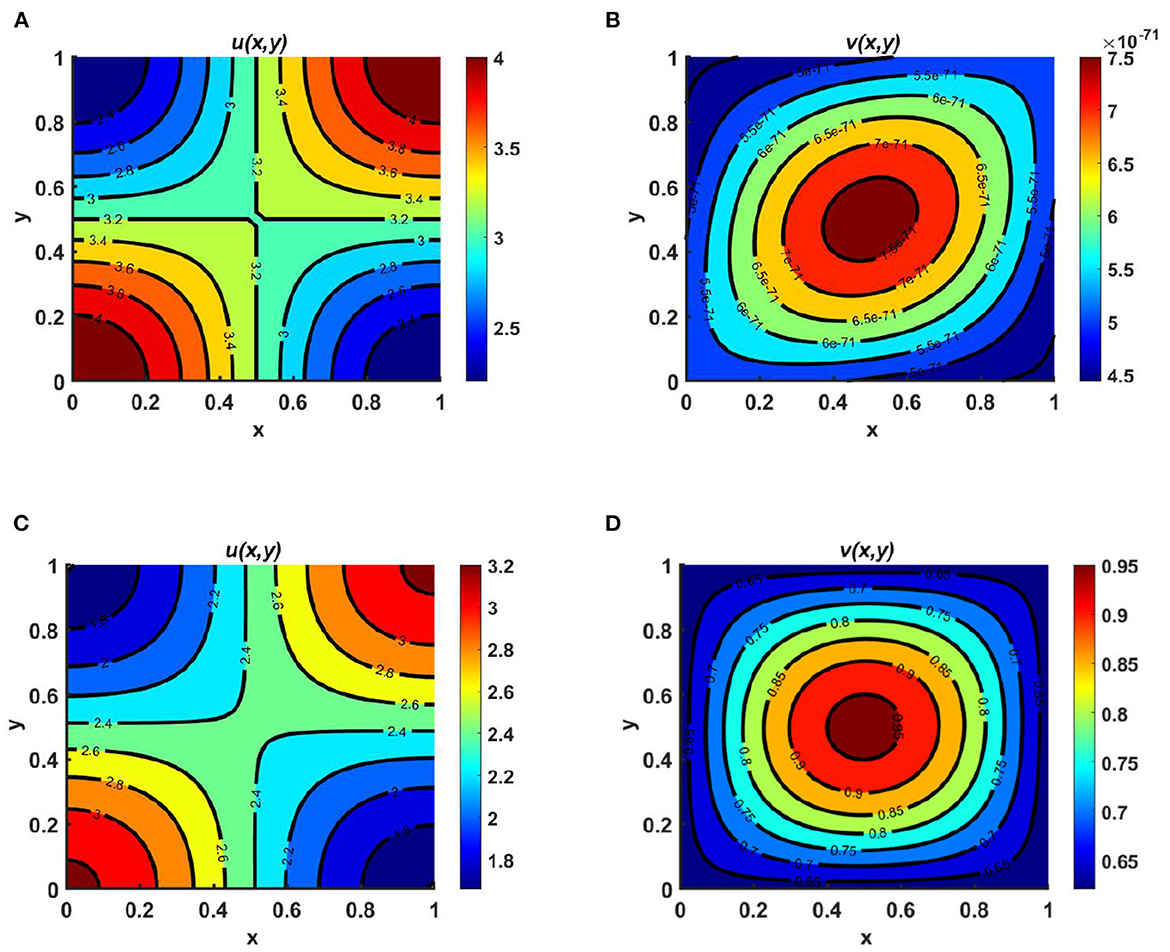
Figure 2. Contour plots for (2.1) with N = 1.8 + sin(πx) sin(πy), r₁ ≡ r₂ ≡ 1.0, d₁ ≡ d₂ ≡ 1.0, (u₀, v₀) = (0.5, 1.75) on ω = (0, 1) × (0, 1) for (A, B) K_u = M = (3.2 + cos(πx) cos(πy)) > K_v = (1.6 + cos(πx) cos(πy)), and (C, D) K_u = K_v = M = 3.2 + cos(πx) cos(πy).

Example 2. Consider the case of a homogeneous environment as K_u = M = 3.2, d₁ ≡ d₂ = 1.0, r₁ ≡ r₂ = 1.0, for fixed N = 1.8 + cos(πx) cos(πy), where in Figures 3A, D K_u = 3.2 > K_v = 2.6, in Figures 3B, E K_u = K_v = 3.2, and in Figures 3C, F K_u = 3.2 < K_v = 4.0. We find that when the carrying capacities are homogeneous and do not depend on the spatial domain, for cases of unequal carrying capacity, one of the semi-trivial equilibrium solutions prevails; in contrast, for cases of equal carrying capacity, scenario with coexistence of the competing species is observed, as mentioned in Remark 2, which correlates with the case of space-dependent carrying capacities, as shown in Figure 2. As we know, carrying capacity is the key element for population growth. In fact, a constant environment can be modeled in the laboratory environment, such as by considering the yeast population in a fixed jar. However, if resources are unevenly distributed over space, spatial diffusion of the species can raise the equilibrium of the total abundance of the population of the environment.

FIGURE 3

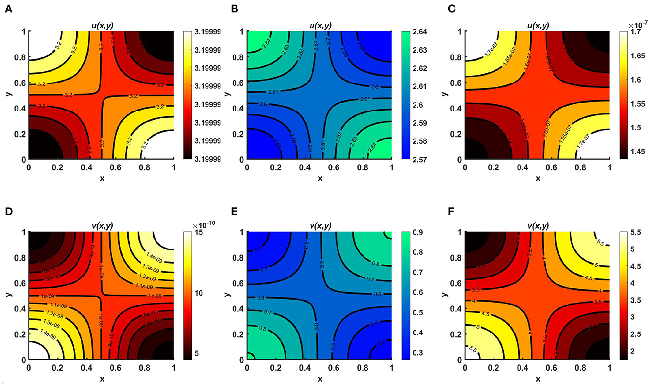
Figure 3. Contour plots for (2.1) with N = 1.8 + cos(πx) cos(πy), r₁ ≡ r₂ ≡ 1.0, d₁ ≡ d₂ ≡ 1.0, (u₀, v₀) = (0.5, 1.75) on ω = (0, 1) × (0, 1) for (A, D) K_u = M = 3.2 > K_v = 2.6, (B, E) K_u = K_v = M = 3.2, and (C, F) K_u = M = 3.2 < K_v = 4.0.

Example 3. We next consider the cases for K_u = M = (1.6 + cos(πx) cos(πy)) < K_v = (3.2 + cos(πx) cos(πy)) with N = 1.8 + sin(πx) sin(πy), d₁ ≡ d₂ ≡ 1.0, (u₀, v₀) = (1.75, 0.5) on ω = (0, 1) × (0, 1) when the intrinsic growth rates of the two species are unequal. If we consider a case of competition between a native and an invasive species, such that r₁ >> r₂ and vice versa, then it is possible to establish additional theoretical results, since the growth of the invasive population is very high. Here, Figure 4 represents equilibrium population density profiles under (2.1). We observe in Figure 4A that when K_v and M are randomly selected, carrying capacity also functions as an important factor that may enable coexistence even in cases of unequal resource distribution between the species. On the other hand, as shown in Figure 4B, when K_u = M > K_v, we find that species u survives and tends to K_u as t → ∞, while the other species v has a very low population density that may go to extinction as time continues.

FIGURE 4

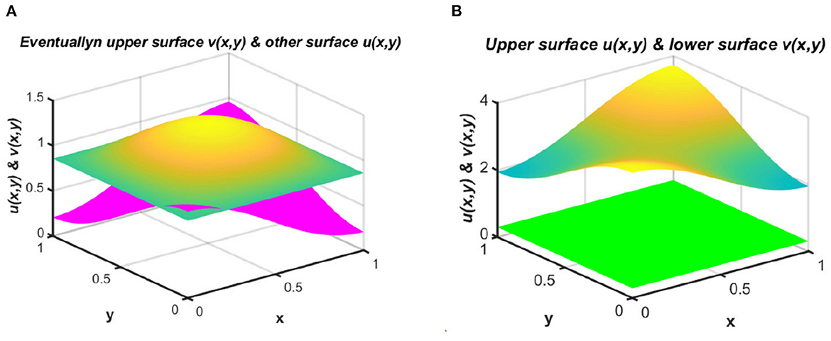
Figure 4. Equilibrium population densities for (2.1) with N = 1.8 + sin(πx) sin(πy), d₁ ≡ d₂ ≡ 1.0, (u₀, v₀) = (1.75, 0.5) when r₁ = 1.0 >> r₂ = 0.01 on ω = (0, 1) × (0, 1) for (A) K_u = M = (1.6 + cos(πx) cos(πy)) < K_v = (3.2 + cos(πx) cos(πy)), and (B) K_u = M = (3.2 + cos(πx) cos(πy)) > K_v = (1.6 + cos(πx) cos(πy)).

Example 4. We now consider K_u = M = (1.6 + cos(πx) cos(πy)) < K_v = (3.2 + cos(πx) cos(πy)), with N = 1.8 + sin(πx) sin(πy) where the diffusion coefficients are same. Figure 5 presents contour plots for u and v for non-negative initial values (u₀, v₀) = (1.75, 0.5), while u is distributed according to per-capita carrying capacity and v follows a resource-based diffusion strategy. We observe in Figures 5A, B that when r₁ = 1.0 >> r₂ = 0.01, the population density of u is notably higher compared to v, and coexistence may occur in cases of higher r₁ as compared to r₂. We also observe that higher population densities of u are found at the bottom-left and top-right corners, while the population density of v is higher in the middle of the contour domain, analogous to N. In contrast, when r₁ << r₂ and K_u < K_v, due to the higher consumption of resources and greater intrinsic growth rate, the population density of v is higher than that of u; see Figures 5C, D.

FIGURE 5

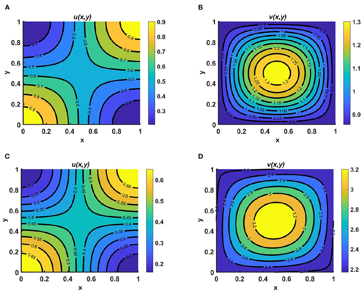
Figure 5. Contour plots for (2.1) for K_u = M = (1.6 + cos(πx) cos(πy)) < K_v = (3.2 + cos(πx) cos(πy)), N = 1.8 + sin(πx) sin(πy), d₁ ≡ d₂ ≡ 1.0, (u₀, v₀) = (1.75, 0.5); in (A, B) r₁ = 1.0 >> r₂ = 0.01, and in (C, D) r₁ = 0.01 << r₂ = 1.0 on ω = (0, 1) × (0, 1).

Example 5. In the next example, we consider cases of unequal carrying capacity while u and v diffuse according to K_u and K_v, respectively, where K_u = M = 2.5 + sin(πx) cos(πy), d₁ ≡ d₂ ≡ 1.0, (u₀, v₀) = (0.5, 0.5), r₁ ≡ r₂ ≡ 1.0 on ω = (0, 1) × (0, 1), with K_v = N = 1.4 + 0.3 sin(πx) sin(πy) in Figures 6A, B, and K_v = N = 3.0 + sin(πx) sin(πy) in Figures 6C, D. We observe that, in all cases, the species which utilizes more resources survives, and the other tends to extinction as time continues, which is justified theoretically in Theorem A1 and Remark A1, respectively (see Appendix). We also find that the population density of u is higher in the bottom-middle region of the contour plot because the values of K_u = M are higher in this region, whereas the population density of v is higher at the center of the domain, as in K_v = N.

FIGURE 6

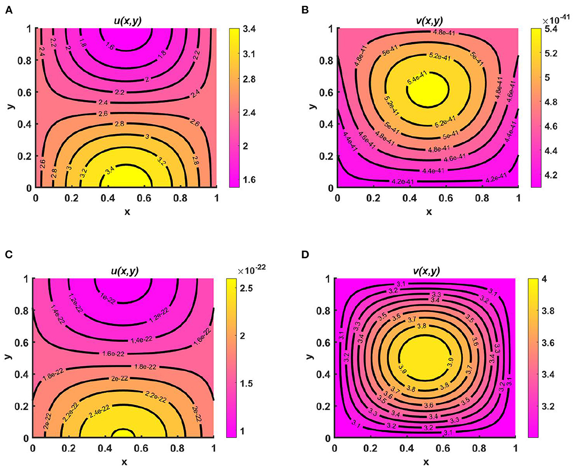
Figure 6. Contour plots for (2.1) with K_u = M = 2.5 + sin(πx) cos(πy), d₁ ≡ d₂ ≡ 1.0, (u₀, v₀) = (0.5, 0.5), r₁ ≡ r₂ ≡ 1.0 on ω = (0, 1) × (0, 1) for (A, B) K_v = N = 1.4 + 0.3 sin(πx) sin(πy), and (C, D) K_v = N = 3.0 + sin(πx) sin(πy).

Example 6. We now turn to the scenario in a numerical setting where resources are limited and both populations are competing for the same food sources in Figures 7A, B. Here, K_u = K_v = 0.5 + 0.3 sin(πx) sin(πy), M = 0.3 + 0.2 cos(πx) cos(πy), N = 0.4 + 0.3 cos(πx) cos(πy), (u₀, v₀) = (0.5, 1.75), r₁ ≡ r₂ ≡ 1.0, d₁ ≡ d₂ ≡ 1.0.We find that coexistence only occurs when both species use the resource-based approach to diffusion. This shows that when two species share certain resources, competitive exclusion can be avoided by using a more advantageous dispersal strategy. However, the contour patterns for both u and v mimic the resource functions, whose maximum and minimum are located at the left and right bottom and top corners of the profile regime. In our forthcoming work, the theoretical outcome of this finding will be presented.

FIGURE 7

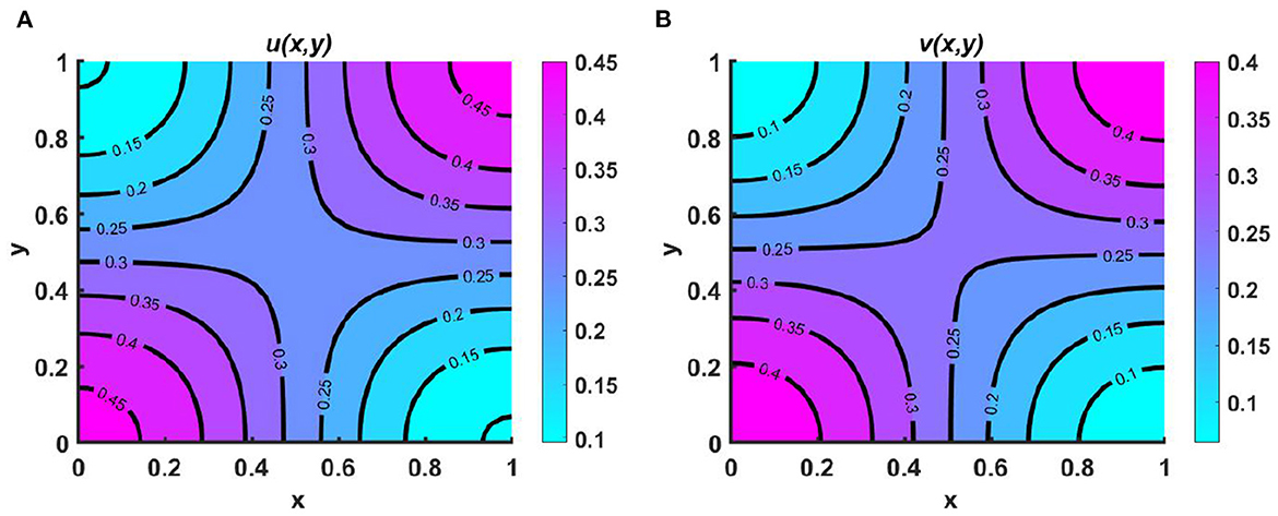
Figure 7. Contour plots of (A) u, and (B) v for (2.1) with K_u = K_v = 0.5 + 0.3 sin(πx) sin(πy), M = 0.3 + 0.2 cos(πx) cos(πy), N = 0.4 + 0.3 cos(πx) cos(πy), (u₀, v₀) = (0.5, 1.75), r₁ ≡ r₂ ≡ 1.0, d₁ ≡ d₂ ≡ 1.0 on ω = (0, 1) × (0, 1).

Example 7. Assume different non-constant carrying capacities, unequal as in Figures 8A, B K_u = 2.5 + cos(πx) cos(πy) > K_v = 1.4 + cos(πx) cos(πy), or equal as in Figures 8C, D K_u = K_v = 2.5 + cos(πx) cos(πy), where M = 1.5 + cos(πx) sin(πy), N = 2.1 + sin(πx) cos(πy), d₁ = 0.1, d₂ = 1.0, (u₀, v₀) = (0.5, 0.5), r₁ ≡ r₂ ≡ 1.0 on ω = (0, 1) × (0, 1). Here, both species u and v diffuse according to their resource function, which is non-proportional to carrying capacity. Here, the carrying capacity of both species is more prominent in the left and right corners, whereas more resources are found for u in the bottom-left and middle-left regions of the domain and for v in the bottom-middle region and right corner of the contour profile. Nevertheless, we observe that in the case of slow diffusion of u, a higher population density is found at the bottom-left and -right corners of the domain, analogous to K_u. This means that, for small values of the diffusion coefficient, the growth of the species depends on the carrying capacity, and a species that undergoes slow diffusion relative to the other will survive in the competition, as stated in Theorem 3; see Figures 8A, B. In contrast, in Figures 8C, D, we observe that if the carrying capacity of both species is equal, then if the species disperse according to resource distribution, they may coexist with unequal diffusion coefficients. It can also be noted that the population density of u is higher in all cases than that of v, which demonstrates that the species that diffuses slowly can survive in the long run as time continues. As we know, when the species diffusion rate is very high, members of the species have a very hard time finding each other and sustaining the population. Under this scenario, it is also difficult for them to protect one another through cooperative defense. This results in notable decline in the species' growth in competition.

FIGURE 8

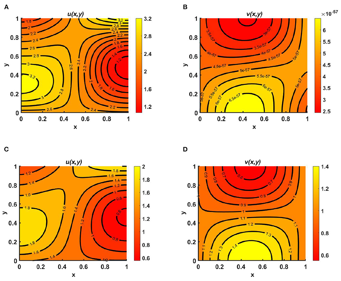
Figure 8. Contour plots for (2.1) with M = 1.5 + cos(πx) sin(πy), N = 2.1 + sin(πx) cos(πy), d₁ = 0.1, d₂ = 1.0, (u₀, v₀) = (0.5, 0.5), r₁ ≡ r₂ ≡ 1.0 on ω = (0, 1) × (0, 1) for (A, B) K_u = 2.5 + cos(πx) cos(πy) > K_v = 1.4 + cos(πx) cos(πy), and (C, D) K_u = K_v = 2.5 + cos(πx) cos(πy).

Example 8. Consider the case of M = 1.6 + cos(πx) cos(πy), N = 1.5 + 0.3 cos(πx) cos(πy), K_u = K_v = K = 1.8 + 0.3 sin(πx) sin(πy), with equal diffusion coefficients and growth rates for both species, where (u₀, v₀) = (1.95, 0.9). Here, in Figures 9A, D we assume K_u = K_v = K = M + N and we observe that coexistence occurrs; this is globally attractive, as stated in Lemma 11, and is known as an ideal free pair. Additionally, in Figures 9B, E we let M = N + K and observe that the population density profile of u is higher compared to that of v and the maximum population densities are found in the middle region or along the saddle point of the contour plot of u which confirms the global existence of (u^*, 0) as stated in Theorem 4. Similarly, in Figures 9C, F we consider N = M + K, for which a higher population density is observed found for v, distributed symmetrically, and the population density of u is found to be very low across the entire domain. This ensures the global existence of (0, v^*), as defined in Remark 4, as time continues. Here, in particular, we have focused on α = β = 1.0.

FIGURE 9

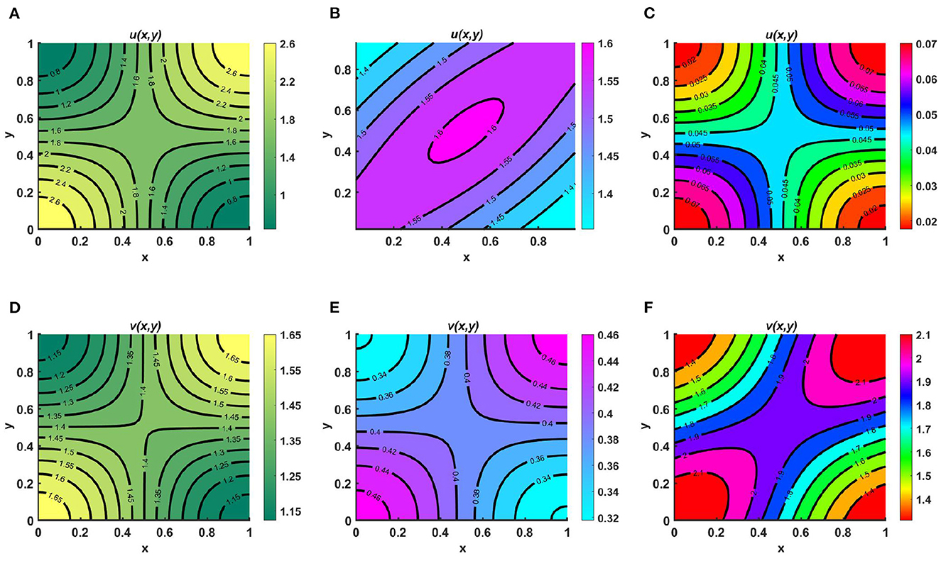
Figure 9. Contour plots for (2.1) with M = 1.6 + cos(πx) cos(πy), N = 1.5 + 0.3 cos(πx) cos(πy), K_u = K_v = K = 1.8 + 0.3 sin(πx) sin(πy), d₁ ≡ d₂ ≡ 1.0, r₁ ≡ r₂ ≡ 1.0, (u₀, v₀) = (1.95, 0.9) on ω = (0, 1) × (0, 1) for (A, D) K_u = K_v = K = M + N, (B, E) M = K + N, and (C, F) N = K + M.

Next, we consider time-dependent functions to demonstrate the existence of periodic solutions and also analyze the model 2.1 for periodic as well as seasonal changes from an ecological perspective.

Example 9. Figures 10A–E represents the periodic behavior of density profiles for u by considering time-varying functions when the carrying capacity of two species are unequal, as in K_u = M = (2.1 + cos(πx) cos(πy))(1.1 + cos(t)) > K_v = (1.5 + cos(πx) cos(πy))(1.1 + sin(t)), N = (2.0 + sin(πx) sin(πy))(1.2 + sin(t)), with equal growth rates and diffusion coefficients for u and v at T = 13.8. Here, for non-negative initial population densities (u₀, v₀) = (1.95, 0.9), u disperses according to per-capita carrying capacity, whereas v is distributed according to its time-dependent resource availability function N. As we know, population growth depends on natural resources, water supply, climate change, land, etc. The population will not have access to the same types of resources at all times during a given time interval; as a result, their growth will not be similar everywhere for a certain period. We notice that at T = 13.6 and T = 13.6 + 2π, the population density profiles represent identical values, and the existence of a unique periodic solution is evident with time growth, which ensures the existence of an attractive positive periodic solution.

FIGURE 10

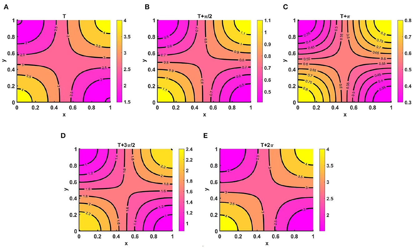
Figure 10. Contour plots of u(t, x, y) for (2.1) with K_u = M = (2.1 + cos(πx) cos(πy))(1.1 + cos(t)) > K_v = (1.5 + cos(πx) cos(πy))(1.1 + cos(t)), N = (2.0 + sin(πx) sin(πy))(1.2 + sin(t)), r₁ ≡ r₂ ≡ 1.0, d₁ ≡ d₂ ≡ 1.0, (u₀, v₀) = (0.5, 1.5) on ω = (0, 1) × (0, 1) at T = 13.8 for (A) T, (B) $T+\frac{\pi }{2}$, (C) T + π, (D) $T+\frac{3\pi }{2}$, and (E) T + 2π.

Example 10. As illustrated in Figure 10, consider the time-dependent functions for K_u = M > K_v (noted in the caption to Figures 11A–E) and N with d₁ ≡ d₂ ≡ 1.0 and r₁ ≡ r₂ ≡ 1.0. We observed the periodic behavior of v at T = 7.1, which is long enough for a time-periodic pattern to emerge. As species v diffuses according to its time-dependent resource function N, the maximum of the density profile is located at the center and is also found to be very low compared to that of u, as stated in Theorem 2, which ensures the global existence of (K_u, 0) as t → ∞.

FIGURE 11

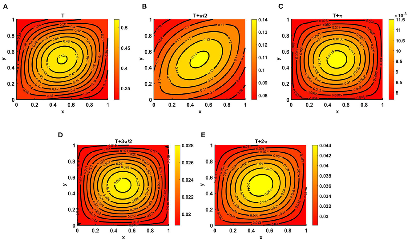
Figure 11. Contour plots of v(t, x, y) for (2.1) with K_u = M = (2.1 + cos(πx) cos(πy))(1.1 + cos(t)) > K_v = (1.5 + cos(πx) cos(πy))(1.1 + cos(t)), N = (2.0 + sin(πx) sin(πy))(1.2 + sin(t)), r₁ ≡ r₂ ≡ 1.0, d₁ ≡ d₂ ≡ 1.0, (u₀, v₀) = (0.5, 1.5) on ω = (0, 1) × (0, 1) at T = 7.1 for (A) T, (B) $T+\frac{\pi }{2}$, (C) T + π, (D) $T+\frac{3\pi }{2}$, and (E) T + 2π.

Example 11. Assume time-dependent functions of the form M = (1.7 + sin(πx) cos(πy))(1.1 + sin(t)) and N = (1.5 + cos(πx) sin(πy))(1.2 + sin(t)), with d₁ ≡ d₂ ≡ 1.0, (u₀, v₀) = (0.6, 0.6) on ω = (0, 1) × (0, 1), where the carrying capacity of both species is considered to be K_u = K_v = (2.5 + cos(πx) cos(πy))(1.1 + sin(t)). In this case, we observe that there is scope for coexistence in the case of unequal intrinsic growth rates, when the species are distributed according to their available resource functions. Additionally, in the contour plots, we note that for both r₁ = 1.0 >> r₂ = 0.01 and r₁ = 0.01 << r₂ = 1.0, the maximum value of u is found in the middle of the bottom region, whereas the maximum for v occurs in the left middle region of the contour profiles. As for the case of relatively large and equal diffusion coefficient values, the dispersion of species depends on the resource function, as both species are diffusing in the direction of their resource functions, which is evident in Figures 12A–D.

FIGURE 12

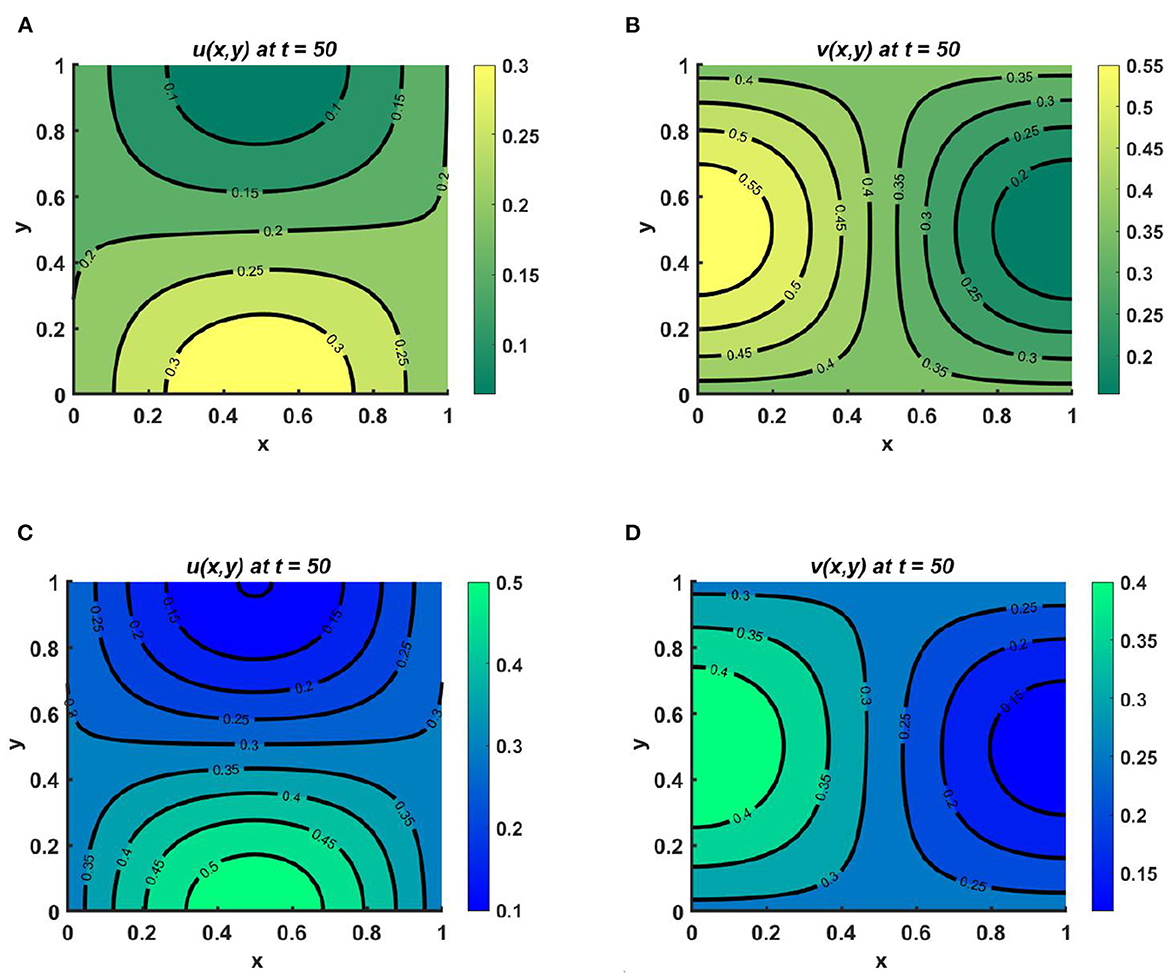
Figure 12. Contour plots for (2.1) with K_u = K_v = (2.5 + cos(πx) cos(πy))(1.1 + sin(t)), M = (1.7 + sin(πx) cos(πy))(1.1 + cos(t)), N = (1.5 + cos(πx) sin(πy))(1.2 + sin(t)), d₁ ≡ d₂ ≡ 1.0, (u₀, v₀) = (0.6, 0.6) on ω = (0, 1) × (0, 1) for (A, B) r₁ = 1.0 >> r₂ = 0.01, and (C, D) r₁ = 0.01 << r₂ = 1.0.

Example 12. Consider M = N = (1.5 + sin(πx) sin(πy))(1.1 + cos(t)), r₁ ≡ r₂ ≡ 1.0 when the carrying capacities of u and v are equal at K_u = K_v = (2.1 + cos(πx) cos(πy))(1.3 + cos(t)) and (u₀, v₀) = (0.6, 0.6) on ω = (0, 1) × (0, 1). We observe from Figures 13A, B that, for fixed d₁ = 1.0 when d₂ = 0.1, species v survives; it is also highlighted here that, for slow diffusion, the growth of the population is dominated by the carrying capacity of the environment. This is evident in Figure 13B, and according to Theorem 5, the global existence of (0, v^*) is clear in the numerical result of Figures 13A, B. On the other hand, when the diffusion coefficients are taken to be d₁ = 1.0 and d₂ = 1.6—that is, for quite large diffusion coefficient values for both species—the diffusion strategies of u and v will depend on the resource functions M and N. However, the maximum population density is found at the center, which is analogous to result for the function M = N, and in this situation, it can also be noted that coexistence is also possible for non-trivial initial population densities on the domain.

FIGURE 13

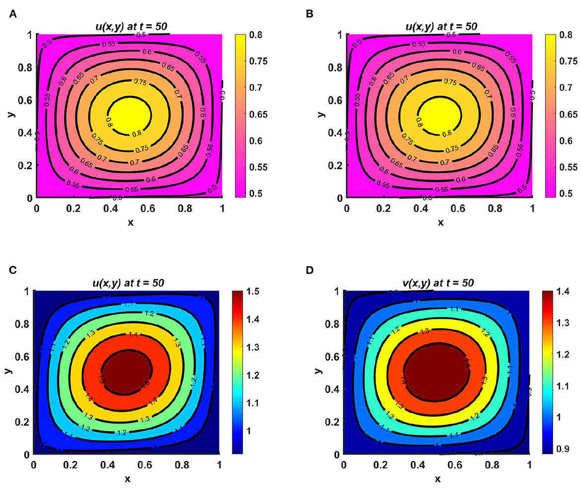
Figure 13. Contour plots for (2.1) with K_u = K_v = (2.1 + cos(πx) cos(πy))(1.3 + cos(t)), M = N = (1.5 + sin(πx) sin(πy))(1.1 + cos(t)), r₁ ≡ r₂ ≡ 1.0, d₁ = 1.0, (u₀, v₀) = (0.6, 0.6) on ω = (0, 1) × (0, 1) for (A, B) d₂ = 0.01, and (C, D) d₂ = 1.6.

7. Conclusion

In this paper, we have reported on the design of a model of competition between a pair of species, in which both species are modeled according to their resource function, which we expect to be more realistic in some scenarios than in others. We examined the global existence of solutions to the model for cases of two species with unequal carrying capacity. We have also considered cases of different dispersion strategies for the two species based on their resource function and carrying capacity. We found that when the resource function is non-proportional to carrying capacity for one species while members of the other are diffusing according to their carrying capacity, the species that consumes more resources will survive in the competition (see Figure 2). However, for the case of both species adopting the same diffusion strategy, while the resource function varies, coexistence is not possible unless the entire environment is homogeneous, which is also valid for the case of proportionality (see Figure 6). The global existence of competitive exclusion in the model is also found to obtain when the carrying capacities and migration strategies of both species are the same, directed toward the individual resource function (see Figure 6). We have also found, based on numerical investigation, that the intrinsic growth rate can play an important factor in population growth for populations that may coexist whether or not resource distributions are unequal (see Figure 5). However, if the competing species select identical dispersal strategies, and dispersal is not proportional to carrying capacity, it appears that the effect of a higher migration rate is to impact the growth rate of the species negatively (see Figure 8). In contrast, an elevated intrinsic growth rate is an optimistic sign that a species may survive in competition (see Figure 4). The temporal and periodic effects on species growth rate that may occur due to seasonal changes have also been illustrated numerically here via contour plots for the model; these plots demonstrate the advantage of selecting different diffusion strategies. The results of the current study can be extended by considering cases of three competing species in symmetric competition. Additionally, harvesting effects could be included in the model in order to show the outcomes for the stability of two competing species in a heterogeneous environment. Finally, one could also study the modified problem for the cases of anomalous diffusion, nonergodicity, and Brownian motion for heterogeneous populations [31, 32].

Data availability statement

The original contributions presented in the study are included in the article/Supplementary material, further inquiries can be directed to the corresponding author.

Author contributions

MK and IZ: conceptualization, software, and formal analysis. IZ, TK, and MK: methodology. IZ: validation, data curation, and original draft preparation. MA and MS: investigation. MA and TK: resources. MK, MS, TK, and MA: review and editing. MK: supervision. All authors have read and agreed to the published version of the manuscript.

Funding

The work by MK was partially supported by the University Grants Commission (UGC) and by the Bose Center for Advanced Study and Research in Natural Sciences, University of Dhaka.

Acknowledgments

The authors acknowledge the reviewers for their comments and suggestions, which significantly improved the quality of the manuscript.

Conflict of interest

The authors declare that the research was conducted in the absence of any commercial or financial relationships that could be construed as a potential conflict of interest.

Publisher's note

All claims expressed in this article are solely those of the authors and do not necessarily represent those of their affiliated organizations, or those of the publisher, the editors and the reviewers. Any product that may be evaluated in this article, or claim that may be made by its manufacturer, is not guaranteed or endorsed by the publisher.

Supplementary material

The Supplementary Material for this article can be found online at: https://www.frontiersin.org/articles/10.3389/fams.2023.1157992/full#supplementary-material

References

1. Conser C. Reaction-diffusion equations and ecological modelling. In: Friedman AA, editor. Book Chapter of the Book: (Evolution and Ecology). Berlin; Heidelberg: Springer (2008).

Google Scholar

2. Dockery J, Hutson V, Mischaikow K, Pernarowski M. The evolution of slow dispersal rates: a reaction diffusion model. J Math Biol. (1998) 37:61–83. doi: 10.1007/s002850050120

CrossRef Full Text | Google Scholar

3. Belgacem F, Cosner C. The effects of dispersal along environmental gradients on the dynamics of populations in heterogeneous environment. Can Appl Math Quart. (1995) 3:379–97.

Google Scholar

4. Cantrell RS, Cosner C, Lou Y. Advection-mediated coexistence of competing species. Proc R Soc Edinburgh Sect A. (2007) 137:497–58. doi: 10.1017/S0308210506000047

CrossRef Full Text | Google Scholar

5. Cantrell RS, Cosner C. Spatial Ecology via Reaction-Diffusion Equations. Wiley Series in Mathematical and Computational Biology. Chichester: John Wiley & Sons (2003).

Google Scholar

6. Williams S, Chow P. Nonlinear reaction-diffusion models for interacting population. J Math Anal Appl. (1978) 62:157–9. doi: 10.1016/0022-247X(78)90227-5

CrossRef Full Text | Google Scholar

7. Cantrell RS, Cosner C, Lou Y. Approximating the ideal free distribution via reaction-diffusion-advection equations. J Differ Eq. (2008) 245:3687–703. doi: 10.1016/j.jde.2008.07.024

CrossRef Full Text | Google Scholar

8. Chakraborty S, Tiwari PK, Misra AK, Chattopadhyay J. Spatial dynamics of a nutrient phytoplankton system with toxic effect on phytoplankton. Math Biosci. (2015) 264:94–100. doi: 10.1016/j.mbs.2015.03.010

PubMed Abstract | CrossRef Full Text | Google Scholar

9. Chakraborty SP, Tiwari K, Sasmal SK, Biswas S, Bhattacharya S, Chattopadhyay J. Interactive effects of prey refuge and additional food for predator in a diffusive predator-prey system. Appl Math Model. (2017) 47:128–40. doi: 10.1016/j.apm.2017.03.028

CrossRef Full Text | Google Scholar

10. Braverman E, Braverman L. Optimal harvesting of diffusive models in a non-homogeneous environment. Nonlinear Anal Theory Methods Appl. (2009) 71:e2173–81. doi: 10.1016/j.na.2009.04.025

CrossRef Full Text | Google Scholar

11. Korobenko L, Braverman E, A. logistic model with a carrying capacity driven diffusion. Can Appl Math Quart. (2009) 17:85–104.

PubMed Abstract

12. Zahan I, Kamrujjaman M, Alim M, Mohebujjaman M, Khan T. Dynamics of heterogeneous population due to spatially distributed parameters and an ideal free pair. Front Appl Math Stat. (2022) 8:949585. doi: 10.3389/fams.2022.949585

CrossRef Full Text | Google Scholar

13. Korobenko L, Braverman E. On evolutionary stability of carrying capacity driven dispersal in competition with regular diffusing populations. J Math Biol. (2014) 69:1181–206. doi: 10.1007/s00285-013-0729-8

PubMed Abstract | CrossRef Full Text | Google Scholar

14. Braverman E, Kamrujjaman M. Competitive-cooperative models with various diffusion strategies. Comput Math Appl. (2016) 72:653–62. doi: 10.1016/j.camwa.2016.05.017

CrossRef Full Text | Google Scholar

15. Braverman E, Kamrujjaman M. Lotka systems with directed dispersal dynamics: Competition and influence of diffusion strategies. Math Biosci. (2016) 279:1–12. doi: 10.1016/j.mbs.2016.06.007

PubMed Abstract | CrossRef Full Text | Google Scholar

16. Oesterheld M, Semmartin M. Impact of grazing on species composition: adding complexity to a generalized model. Austral Ecol. (2011) 36:881–90. doi: 10.1111/j.1442-9993.2010.02235.x

CrossRef Full Text | Google Scholar

17. Follak S, Strauss G. Potential distribution and management of the invasive weed Solanum Carolinense in Central Europe. Weed Res. (2010) 50:544–52. doi: 10.1111/j.1365-3180.2010.00802.x

CrossRef Full Text | Google Scholar

18. Saether BE, Lillegard M, Groton V, Derever MC, Engen S, Nudds TD, et al. Geographical gradients in the population dynamics of North-America Prairie ducks. Anim Ecol J. (2008) 77:869–82. doi: 10.1111/j.1365-2656.2008.01424.x

PubMed Abstract | CrossRef Full Text | Google Scholar

19. Cantrell RS, Cosner C, Lou Y. Evolution of dispersal and the ideal free distribution. Math Biosci Eng. (2010) 7:17–36. doi: 10.3934/mbe.2010.7.17

PubMed Abstract | CrossRef Full Text | Google Scholar

20. Braverman E, Kamrujjaman M, Korobenko L. Competitive spatially distributed population dynamics model: does diversity in diffusion strategies promote coexistance? Math Biosci. (2015) 264:63–73. doi: 10.1016/j.mbs.2015.03.004

PubMed Abstract | CrossRef Full Text | Google Scholar

21. Kamrujjaman M. Directed vs. regular diffusion strategy: evolutionary stability analysis of a competition model and an ideal free pair. Differ Eq Appl. (2019) 11:267–90. doi: 10.7153/dea-2019-11-11

CrossRef Full Text | Google Scholar

22. Kamrujjaman M. Interplay of resource distributions and diffusion strategies for spatially heterogeneous populations. J Math Model. (2019) 7:175–98. doi: 10.22124/jmm.2019.11734.1208

CrossRef Full Text | Google Scholar

23. Zahan I, Kamrujjaman M, Tanveer S. Mathematical study of a resource-based diffusion model with Gilpin Ayala growth and harvesting. Bull Math Biol. (2022) 84:1202022. doi: 10.1007/s11538-022-01074-8

PubMed Abstract | CrossRef Full Text | Google Scholar

24. Pao CV. Nonlinear Parabolic and Elliptic Equations. New York, NY: Plenum (1992).

Google Scholar

25. Smith HL. Monotone dynamical systems: an Introduction to the theory of competitive and cooperative system. Am Math Soc. (2008) 41. doi: 10.1090/surv/041

CrossRef Full Text | Google Scholar

26. Lam KY, Liu S, Lou Y. Selected topics on reaction-diffusion-advection models from spatial ecology. Math Appl Sci Eng. (2020) 1:150–80. doi: 10.5206/mase/10644

CrossRef Full Text | Google Scholar

27. Korobenko L, Kamrujjaman M, Braverman E. Persistence and extinction in spatial model with a carrying capacity driven diffusion and harvesting. J Math Anal Appl. (2013) 399:352–68. doi: 10.1016/j.jmaa.2012.09.057

CrossRef Full Text | Google Scholar

28. Dancer EN. Positivity of maps and applications. Topol Nonlinear Anal. (1995) 15:303–40. doi: 10.1007/978-1-4612-2570-6_4

CrossRef Full Text | Google Scholar

29. Hsu S, Smith H, Waltman P. Competitive exclusion and coexistence for competitive systems on ordered Banach spaces. Trans Am Math Soc. (1996) 348:4083–94. doi: 10.1090/S0002-9947-96-01724-2

CrossRef Full Text | Google Scholar

30. Gilbarg D, Trudinge NS. Elliptic Partial Differential Equations of Second Order. 2nd ed. Berlin: Springer (1983).

Google Scholar

31. Wang W, Cherstvy AG, Liu X, Metzler R. Anomalous diffusion and nonergodicity for heterogeneous diffusion processes with fractional Gaussian noise. Phys Rev E. (2020) 102:012146. doi: 10.1103/PhysRevE.102.012146

PubMed Abstract | CrossRef Full Text | Google Scholar

32. Wang W, Cherstvy AG, Kantz H, Metzler R, Sokolov IM. Time averaging and emerging nonergodicity upon resetting of fractional Brownian motion and heterogeneous diffusion processes. Phys Rev E. (2021) 104:024105. doi: 10.1103/PhysRevE.104.024105

PubMed Abstract | CrossRef Full Text | Google Scholar