Individual-based multiscale model for foot-and-mouth disease

The study of infectious disease dynamics across various hierarchical levels and scales of organization has gained significant attention in the realm of mathematical biology. We develop an individual-based network multiscale model of foot-and-mouth disease (FMD) in cattle based on the replication-transmission relativity theory at whole living organism level. An important feature of individual-based network multiscale models is that they incorporate heterogeneity in [i.] host susceptibility to infection, [ii.] the ability of hosts to transmit pathogen to other hosts, [iii.] host immune response, and [iv.] host behaviour. Numerical simulations are conducted to demonstrate the influence of model parameters designated for controlling, eliminating, and eradicating FMD. Results indicate that microscale parameters such as the clearance rate of virus, ω_i and the macroscale parameters like the transmission rate between the cattle, β_ij are crucial for implementing interventions (vaccination and quarantine respectively). Additionally, the analysis of the network degree distribution indicates the absence of hubs due to lack of a heavy tail on the histogram.

1 Introduction

The study of infectious disease dynamics across various hierarchical levels and scales of organization has gained significant attention in the realm of mathematical biology. This surge in interest has been facilitated by an innovative approach known as multiscale modeling, which provides fresh perspectives on the dynamics of infectious disease systems. The fundamental ideas of multiscale modeling of infectious disease systems have been elucidated by recent publications [1–5]. Further, these ideas have been underpinned by a biological relativity theory that provides a theoretical framework for development of such multiscale models [6]. A key postulate of this biological relativity theory is that any infectious disease system is organized into seven main levels of hierarchical level of organization namely: the cell level, the tissue level, the organ level/microcommunity level, the microecosystem level, the host level, the macrocommunity level, and the macroecosystem level [3]. The dynamics of pathogen from one scale of organization to another at any of these seven levels of organization necessarily involves a replication-transmission multiscale cycle of pathogen replication at microscale and pathogen transmission at macroscale. Another fundamental postulate of this biological relativity theory is that at any of these levels of organization, the multiscale models that can be developed fall into five main categories [3]: (i) the hybrid multiscale models (HMSMs), (ii) nested multiscale models (NMSMs), (iii) embedded multiscale models (EMSMs), (iv) individual-based multiscale models (IMSMs), and (iv) coupled multiscale models (CMSMs). However, the category of individual-based multiscale models is further classified into four main classes namely [3]: network modeling individual-based multiscale models (NETW-IMSMs), empirical data modeling individual-based multiscale models (EMPI-IMSMs), simulation modeling individual-based multiscale models (SIMU-IMSMs), and hybrid individual-based multiscale models (BRID-IMSMs). This study is about the development of network modeling individual-based multiscale models. Further, network modeling individual-based multiscale models can be formulated using any of the five graph-theoretic techniques which include: lattice network models, scale-free network models, spatial network models, random network models and smallworld network models [7]. Applications of network models include transportation and mobility networks, internet, mobile phone networks, power grids, social and contact networks, neural networks. In the realm of infectious diseases, a network consists of nodes (vertices) and links (edges), where nodes represent individuals (humans, animals, plants, computers, farms, patches, etc.) who are either susceptible to infection or capable of transmitting infections, and links denote interactions between individuals that may facilitate transmission.

This study presents an individual-based network model of foot-and-mouth disease (FMD) based on the replication-transmission relativity theory [6]. The multiscale model which integrates the within-host and between-host dynamics of FMD in cattle. An important feature of individual-based network modeling multiscale models is heterogeneity in (i) host susceptibility to infection, (ii) the ability of hosts to transmit pathogen to other hosts, (iii) host immune response, (iv) host behavior [5]. Furthermore, the within-host submodel is implemented to describe the entire infectious disease system across both the within-host scale and between-host scale. Therefore, the main aim of this study is to establish the influence of heterogeneity, using an individual-based spatial network multiscale model, on disease dynamics for an infection. To the best of our knowledge, there is currently no individual-based multiscale network model in the existing literature that utilizes the replication-transmission relativity theory and considers the interaction between two scales at any level of an infectious disease system. The dynamics of FMD in the cattle population consists of various transmission routes of FMDV at between-host scale including air-borne spread, animal-to-animal contact and contamination of the environment [8, 9]. Globally, FMD is known to have caused major losses in the agricultural sector as well as tourism [10]. In Africa, FMD is regarded as the most significant economic animal illness impacting regional trade in livestock, wildlife, and various agricultural goods [11]. The usual control measures of FMD include (i) movement restriction of animals, animal products and fomites; (ii) quarantine; (iii) culling of detected infected animals, (iv) surveillance and tracing to establish the source and path of the infection, and (v) vaccination [12] with the latter having a significant impact in controlling FMD [13, 14]. However, all these control measures have their own limitations in combating FMD in cattle [15]. A key aspect of multiscale dynamics is the replication-transmission relativity theory which states that at any hierarchical level of organization of an infectious disease system there is no priviledge or absolute scale which will determine disease dynamics, only interactions between the microscale and macroscale [6].

Previously, multiscale modeling of FMD in cattle at host level has been established. This was done by formulating hybrid multiscale models (HMSMs) such as Bradhurst et al. [16] and individual-based multiscale models (IMSMs) such as Kao et al. [17] and Kostova-Vassilevska [18]. The contributions made by the HMSMs in Bradhurst et al. [16] and IMSMs in Kao et al. [17] and Kostova-Vassilevska [18] have given new insights into the impact of health interventions against FMD, however, there are some vital limitations of these multiscale categories when compared with the individual-based network modeling multiscale model described in this paper. The HMSMs cannot be utilized to establish heterogeneity in (i) host susceptibility to infection, (ii) the ability of hosts to transmit pathogen to other hosts, (iii) host immune response, and (iv) host behavior. On the other hand, the IMSMs in Kao et al. [17] and Kostova-Vassilevska [18] did not address the reciprocal influence of the microscale and macroscale at any hierarchical level of infectious disease systems. It is important to note that some of the mathematical models of FMD infection are single-scale models [18–20]. However, single scale models are only confined to one component of the replication-transmission multiscale cycle of infectious disease systems.

The rest of the contents of this paper is organized in the following way. In Section 2, we present the network modeling individual-based model for FMD in cattle. The mathematical analysis of the network modeling individual-based model is done in Section 3. In Section 4, the network modeling individual-based model is analyzed numerically to validate some of the analytical results obtained in Section 3. Finally, the conclusions of the study are presented in Section 5.

2 The individual-based multiscale model for FMD

The formulation of this model involves differential equations illustrating the initial transmission of FMDV taking into account immune response and then placing the cattle population in a spatial network. The model we develop is an extension of the wihin-host model developed by Howey et al. [20], who investigated the dynamics of this disease in cattle. For each individual i there is interplay between antibody, A_i, virions in blood, V_i, interferon, I_i, uninfected epithelial cells, U_i, infected epithelial cells, F_i, non-infectious material denoted by J_i, virus-antibody complexes, C_i and protected cells, P_i. Given below is the set of differential equations:

$\begin{array}{ll}\frac{d{V}_i}{dt}={\zeta }_i{F}_i-{\varphi }_{A_i}{\omega }_i{V}_i+{\displaystyle \sum _{i\ne j,j=1}^n}{\beta }_{ij}{V}_j,& (1)\end{array}$

$\begin{array}{ll}\frac{d{F}_i}{dt}={ϵ}_i{U}_i{V}_i-{\zeta }_i{F}_i,& (2)\end{array}$

$\begin{array}{ll}\frac{d{U}_i}{dt}=-{\kappa }_i{U}_i\left(I_i-\frac{{\mu }_i}{{\xi }_i}\right),& (3)\end{array}$

$\begin{array}{ll}\frac{d{P}_i}{dt}={\kappa }_i{U}_i\left(I_i-\frac{{\mu }_i}{{\xi }_i}\right),& (4)\end{array}$

$\begin{array}{ll}\frac{d{I}_i}{dt}={\mu }_i-{\xi }_i{I}_i+{\varphi }_{U_i}(U){\eta }_i{C}_i,& (5)\end{array}$

$\begin{array}{ll}\frac{d{A}_i}{dt}={\varphi }_{V_i}(V,J){\varphi }_{A_i},& (6)\end{array}$

$\begin{array}{ll}\frac{d{C}_i}{dt}={\varphi }_{A_i}{\omega }_i(V_i+J_i)-{\sigma }_i{C}_i,& (7)\end{array}$

$\begin{array}{ll}\frac{d{J}_i}{dt}={\gamma }_i{\zeta }_i{F}_i-{\varphi }_{A_i}{\omega }_i{J}_i& (8)\end{array}$

where

$\begin{array}{l}{\beta }_{ij}=\beta (1-{\delta }_{ij})e^{-\alpha |i-j|},\end{array}$

δ_ij is Kronecker's delta, β and α are non-negative. Small values of α implies a widespread influence of infection while bigger values of α implies local spread. The elements β_ji of the transmission matrix B, representing the strength of transmission from j to i depend on spatial factors. β represents the overfall strength of transmission [21].

The model is illustrated by the schematic diagram in Figure 1 and the model variables are summarized in Table 1. Equation 1 of multiscale model system represents the concentration of infectious virion in blood. The first term on the right hand side represents the infected epithelial cells that burst to release more infectious virion in the blood. The second term is the infectious virion cleared as it complexes with antibody. The Equation Equation 2 of multiscale model system represents the infected epithelial cells created at a rate of ϵ_iU_iV_i. The last part of Equation 2 is the infected epithelial cells which burst to become infectious virion. Equation 3 of multiscale model system represents proportion of the uninfected epithelial cells that become protected by interferon from infection when interferon is above background level, μ_i/ξ_i. Equation 4 of multiscale model system represents the proportion of protected epithelial cells. These cells are recruited from uninfected cells when interferon is above background level, μ_i/ξ_i. Equation 5 of multiscale model system represents interferon which is produced at rate, η_iC_i, corresponding to the virus-antibody complexes, C_i. Equation 6 of multiscale model system represents antibody production in relation to the virus that must be neutralized. Equation 7 of multiscale model system represents infectious virion and non-infectious material that has been neutralized by antibody. The last part of Equation 7 is the clearance of virus-antibody complex. In Equation 8 of multiscale model system the first part is the recruitment of non-infectious material from infected cells. The second part is the non-infectious material that is neutralized by antibody.

Figure 1

Figure 1. Schematic diagram of FMD dynamics in a network. For each individual i there is interplay between antibody, A_i, virions in blood, V_i, interferon, I_i, uninfected epithelial cells, U_i, infected epithelial cells, F_i, non-infectious material denoted by J_i, virus-antibody complexes, C_i and protected cells, P_i.

Table 1

Table 1. Description of individual-based multiscale model variables for the ith individual.

3 Mathematical analysis of the individual-based multiscale model of FMD dynamics

3.1 Feasible region of the model

The model that we formulate has to be biologically meaningful. Therefore, we establish the non-negativity and boundedness of all the state variables as well as their solutions, respectively, in the region Φ, where

$\begin{array}{ll}\text{Φ}=\left\{(U_i,V_i,F_i,P_i,I_i,A_i,C_i,J_i)\in {ℝ}_{+}^8\right\},i=1,..,n& (9)\end{array}$

3.1.1 Positivity of solutions

Theorem 3.1. A non-negative solution (V_i(t), F_i(t), U_i(t), P_i(t), I_i(t), A_i(t), C_i(t), J_i(t)) exists for all t ≥ 0

Proof. The positivity of solutions of the multiscale model system (Equations 1–8) is proved using the integrating factor technique. We consider Equation 1 in the multiscale model system

$\begin{array}{ll}\frac{d{V}_i}{dt}={\zeta }_i{F}_i-{\varphi }_{A_i}{\omega }_i{V}_i+{\displaystyle \sum _{j=1,i\ne j}^n}{\beta }_{ij}{V}_j& (10)\end{array}$

We re-write Equation 10 as follows

$\begin{array}{ll}\frac{d{V}_i}{dt}+{\varphi }_{A_i}{\omega }_i{V}_i={\zeta }_i{F}_i+{\displaystyle \sum _{j=1,i\ne j}^n}{\beta }_{ij}{V}_j& (11)\end{array}$

The integrating factor for Equation 11 is

$\begin{array}{ll}\text{Integrating factor (IF)}=e^{{\displaystyle {\int }_0^t}{\varphi }_{A_i}{\omega }_{i}ds}=e^{{\varphi }_{A_i}{\omega }_{i}t}& (12)\end{array}$

When we multiply Equation 11 by the integrating factor $e^{{\varphi }_{A_i}{\omega }_{i}t}$ to get

$\begin{array}{ll}{e}^{{\varphi }_{A_i}{\omega }_{i}t}\frac{d{V}_i}{dt}+e^{{\varphi }_{A_i}{\omega }_{i}t}{\varphi }_{A_i}{\omega }_i{V}_i=e^{{\varphi }_{A_i}{\omega }_{i}t}\left({\zeta }_i{F}_i+{\displaystyle \sum _{j=1,i\ne j}^n}{\beta }_{ij}{V}_j\right)& (13)\end{array}$

From the product rule we obtain

$\begin{array}{ll}\frac{d}{dt}(e^{{\varphi }_{A_i}{\omega }_{i}t}.V_i)=e^{{\varphi }_{A_i}{\omega }_{i}t}\left({\zeta }_i{F}_i+{\displaystyle \sum _{j=1,i\ne j}^n}{\beta }_{ij}{V}_j\right)& (14)\end{array}$

We integrate both sides of Equation 14 with respect to t and obtain

$\begin{array}{ll}{e}^{{\varphi }_{A_i}{\omega }_{i}t}.V_i(t)=e^{{\varphi }_{A_i}{\omega }_i(0)}.V_i(0)+{\displaystyle {\int }_0^t}{e}^{{\varphi }_{A_i}{\omega }_{i}s}\left({\zeta }_i{F}_i(s)+{\displaystyle \sum _{j=1,i\ne j}^n}{\beta }_{ij}{V}_j(s)\right)ds& (15)\end{array}$

Dividing both sides of Equation 15 by the integrating factor $e^{{\varphi }_{A_i}{\omega }_{i}t}$ we get

$\begin{array}{ll}{V}_i(t)=e^{-{\varphi }_{A_i}{\omega }_{i}t}.\left[V_i(0)+{\displaystyle {\int }_0^t}{e}^{{\varphi }_{A_i}\omega s}\left({\zeta }_i{F}_i(s)+{\displaystyle \sum _{j=1,i\ne j}^n}{\beta }_{ij}{V}_j(s)\right)ds\right]\ge 0& (16)\end{array}$

Similarly, the results for Equations 2, 5, 7, and 8 of the multiscale model systemcan also be obtained by the integrating factor technique.

We now consider Equation 3 of the multiscale model system

$\begin{array}{ll}\frac{d{U}_i}{dt}=-{\kappa }_i{U}_i\left(I_i-\frac{{\mu }_i}{{\xi }_i}\right)& (17)\end{array}$

Positivity of the solution of Equation 3 of the multiscale model system is proved using the separation of variables as follows

$\begin{array}{ll}\frac{1}{U_i}d{U}_i=-{\kappa }_i\left(I_i-\frac{{\mu }_i}{{\xi }_i}\right)dt& (18)\end{array}$

We integrate both sides of Equation 14 with respect to t to get

$\begin{array}{ll}{\displaystyle {\int }_0^t}\frac{1}{U_i}d{U}_i=-{\kappa }_i{\displaystyle {\int }_0^t}\left(I_i(s)-\frac{{\mu }_i}{{\xi }_i}\right)ds& (19)\end{array}$

Integrating the left side gives

$\begin{array}{ll}ln\frac{U_i(t)}{U_i(0)}=-{\kappa }_i{\displaystyle {\int }_0^t}\left(I_i(s)-\frac{{\mu }_i}{{\xi }_i}\right)ds& (20)\end{array}$

Removing ln we have the following result

$\begin{array}{ll}{U}_i(t)=U_i(0)exp\left\{-{\kappa }_i{\displaystyle {\int }_0^t}\left(I_i(s)-\frac{{\mu }_i}{{\xi }_i}\right)ds\right\}\ge 0& (21)\end{array}$

Positivity of Equation 4 of the multiscale model systemis proved by integrating both sides of Equation 22.

$\begin{array}{ll}\frac{d{P}_i}{dt}={\kappa }_i{U}_i\left(I_i-\frac{{\mu }_i}{{\xi }_i}\right)& (22)\end{array}$

This gives

$\begin{array}{ll}{\displaystyle {\int }_0^t}d{P}_i={\displaystyle {\int }_0^t}{\kappa }_i{U}_i(s)\left(I_i(s)-\frac{{\mu }_i}{{\xi }_i}\right)ds& (23)\end{array}$

We get the following result

$\begin{array}{ll}{P}_i(t)=P_i(0)+{\displaystyle {\int }_0^t}{\kappa }_i{U}_i(s)\left(I_i(s)-\frac{{\mu }_i}{{\xi }_i}\right)ds\ge 0& (24)\end{array}$

since the protected cells P_i are recruited from uninfected cells when interferon I_i is above background level, $\frac{{\mu }_i}{{\xi }_i}$, that is, $I_i(t)>\frac{{\mu }_i}{{\xi }_i}$. Similarly, the result of Equation 6 of the multiscale model system is a positive solution since both ϕ_Vi(V, J) and ϕ_Ai are positive constants.

Consequently, V_i(t) ≥ 0, F_i(t) ≥ 0, U_i(t) ≥ 0, P_i(t) ≥ 0, I_i(t) ≥ 0, A_i(t) ≥ 0, J_i(t) ≥ 0 and C_i(t) ≥ 0 for all time t > 0.

3.1.2 Boundedness of solutions

We show that all eight equations are ultimately bounded for t ≥ 0. From the Equation 3 of the multiscale model system, the viral infection reduces the population of the uninfected cells so that at the onset of the infection, the population of uninfected cells must be greater or equal to the total cell population at t > 0. The population of uninfected cells is also reduced as a proportion of the cells become protected. Equation 5 of the multiscale model system reduces to $\frac{{\mu }_i}{{\xi }_i}$ while the remaining equations reduce to zero at disease-free equilibrium.

This leaves Equation 3 of the multiscale model system given by

$\begin{array}{ll}\frac{d{U}_i}{dt}=-{\kappa }_i{U}_i\left(I_i-\frac{{\mu }_i}{{\xi }_i}\right)& (25)\end{array}$

$\begin{array}{ll}{U}_i(t)=U_i(0)exp\left\{-{\kappa }_i{\displaystyle {\int }_0^t}\left(I_i(s)-\frac{{\mu }_i}{{\xi }_i}\right)ds\right\}& (26)\end{array}$

Initially, the interferons equal to $\frac{{\mu }_i}{{\xi }_i}$. However, when the interferons are above background level, that is, $\frac{{\mu }_i}{{\xi }_i}$ is implies that $\left(I_i(s)-\frac{{\mu }_i}{{\xi }_i}\right)>0$. Therefore, from Equation 26 we have

$\begin{array}{ll}{\displaystyle \underset{t\to \infty }{lim}}sup{U}_i(t)\le {\displaystyle \underset{t\to \infty }{lim}}sup{U}_i(0)=U_i(0)=N_i& (27)\end{array}$

Thus, the multiscale model system (Equations 1–8) is bounded above by N_i and bounded below by 0. Since the multiscale model system (Equations 1–8) is positive and bounded, it is well-posed (epidemiologically and mathematically) in the region Φ.

3.2 Determination of disease free equilibrium and its stability

3.2.1 The disease-free equilibrium point

In order to establish the disease-free equilibrium point of the multiscale model system in the disease compartment we set the right-hand side of the Equations 1–8 of multiscale model system to zero. When the equilibrium is disease-free then infectious virions in the blood of an individual will not exist resulting no transmission of infection. Therefore, the disease-free equilibrium of the multiscale model system (Equations 1–8) is given by

$\begin{array}{l}{E}^0=(U_i^0,V_i^0,F_i^0,P_i^0,I_i^0,A_i^0,C_i^0,J_i^0)=\left(N_i,0,0,0,\frac{{\mu }_i}{{\xi }_i},0,0,0\right),\\ i=1,...,n& (28)\end{array}$

where N_i, a constant, is the initial number of uninfected epithelial cells. $A_i^0=0$ since this is the time during which virus replication is not yet observable.

3.2.2 The model reproductive number

The reproductive number, ${\mathcal{R}}_0$ is described as the average number of secondary infections generated by an infectious individual host brought into an entirely susceptible population [22, 23]. It is an important parameter which helps to examine outbreak of disease. For the vast majority of disease outbreaks, if ${\mathcal{R}}_0<1$, this implies that the outbreak dies out, while when ${\mathcal{R}}_0>1$, this implies that the outbreak persists. For FMDV infection in cattle, ${\mathcal{R}}_0$ describes the anticipated number of cattle FMDV infections generated by an individual animal throughout the whole cycle of virulence of the animal placed in a totally susceptible cattle population. Hence, ${\mathcal{R}}_0$ quantifies transmission of FMDV from animal to animal. In order to evaluate the basic reproductive number we implement the next generation operator approach [22]. The multiscale model system (Equations 1–8) can be expressed as follows:

$\begin{array}{ll}\{\begin{array}{c}\frac{dX}{dt}=f(X,Y,Z),\\ \frac{dY}{dt}=g(X,Y,Z),\\ \frac{dZ}{dt}=h(X,Y,Z),\end{array}& (29)\end{array}$

where

$\begin{array}{r}X=(U_i,P_i)\\ Y=(J_i,C_i,A_i,I_i)\\ Z=(F_i,V_i).\end{array}$

The elements of X stand for the number of susceptibles as well as other groups of non-infectious individuals. The elements of Y stand for the number of infected individuals who are unable to transmit the disease. The elements of Z stand for the number of infected individuals able to transmit the disease. We define $\tilde{g}(X^{*},Z)$ from Castillo-Chavez et al. [22] by

$\tilde{g}(X^{*},Z)=\frac{{ϵ}_i{N}_i{V}_i}{{\zeta }_i}$

Suppose $A=D_{Z}h(X^{*},\tilde{g}(X^{*},0),0)$ so that A is expressed as A = M−D.

Then from Equations 1 and 2 of multiscale model system A becomes

$\begin{array}{ll}A=\left[\begin{array}{cc}{\displaystyle \underset{i\ne j,j=1}{\sum ^n}}{\beta }_{ij}-{\varphi }_{A_i}{\omega }_i& {\zeta }_i\\ {ϵ}_i{N}_i& -{\zeta }_i\end{array}\right]& (30)\end{array}$

with

$\begin{array}{ll}M=\left[\begin{array}{cc}{\displaystyle \underset{i\ne j,j=1}{\sum ^n}}{\beta }_{ij}& 0\\ {ϵ}_i{N}_i& 0\end{array}\right]& (31)\end{array}$

and

$\begin{array}{ll}D=\left[\begin{array}{cc}{\varphi }_{A_i}(t){\omega }_i& {\zeta }_i\\ 0& -{\zeta }_i\end{array}\right]& (32)\end{array}$

Therefore, the inverse of matrix D is

$\begin{array}{ll}{D}^{-1}=\left[\begin{array}{cc}\frac{1}{{\varphi }_{A_i}{\omega }_i}& \frac{1}{{\varphi }_{A_i}{\omega }_i}\\ 0& \frac{1}{{\zeta }_i}\end{array}\right]& (33)\end{array}$

When we multiple M and D⁻¹ we get

$\begin{array}{ll}M{D}^{-1}=\left[\begin{array}{cc}{\displaystyle \underset{i\ne j,j=1}{\sum ^n}}{\beta }_{ij}& 0\\ {ϵ}_i{N}_i& 0\end{array}\right]\left[\begin{array}{cc}\frac{1}{{\varphi }_{A_i}{\omega }_i}& \frac{1}{{\varphi }_{A_i}{\omega }_i}\\ 0& \frac{1}{{\zeta }_i}\end{array}\right]& (34)\end{array}$

This simplifies to

$\begin{array}{ll}M{D}^{-1}=\left[\begin{array}{cc}\frac{{\displaystyle \underset{i\ne j,j=1}{\sum ^n}}{\beta }_{ij}+{ϵ}_i{N}_i}{{\varphi }_{A_i}{\omega }_i}& 0\\ \frac{{ϵ}_i{N}_i}{{\zeta }_i}& 0\\ \end{array}\right]& (35)\end{array}$

${\mathcal{R}}_0$ is the spectral radius (dominant eigenvalue) of MD⁻¹ and so we have the following expression

$\begin{array}{l}{\mathcal{R}}_0=\rho (M{D}^{-1})\end{array}$

$\begin{array}{ll}{\mathcal{R}}_{0i}=\frac{{\displaystyle \underset{i\ne j,j=1}{\sum ^n}}{\beta }_{ij}+{ϵ}_i{N}_i}{{\varphi }_{A_i}{\omega }_i}& (36)\end{array}$

$\begin{array}{ll}{\mathcal{R}}_0=max\left\{{\mathcal{R}}_{0i}\right\}& (37)\end{array}$

Therefore, the reproductive number ${\mathcal{R}}_0$, is composed of microscale and macroscale disease parameters ϵ, ω and β_ij respectively. When we refer to the formulation for ${\mathcal{R}}_0$ from Equation 36 we can gather the following.

(i) The macroscale transmission parameter, β_ij from Equation 36 which represents the strength of transmission between individuals j and i due to their separation distance, contributes to the spread of FMD infection. The constant α controls the strength of transmission such that when α is small then the probability of transmission β_ij from j to i is high and for bigger values of α the transmission between individuals is low.

(ii) The microscale transmission parameters ϵ_i, the infection rate of epithelial cells as well as ω_i, which controls rate of clearance of virus from Equation 36 have an effect on the spread of virus. The immune response, including ω_i, helps to reduce FMDV transmission.

Therefore, it can be concluded that both macroscale and microscale factors have an impact on the spread of FMDV.

3.2.3 Local stability of the disease free equilibrium (DFE)

In this section we establish the local stability of disease-free equilibrium of the multiscale model system (Equations 1–8).

$\begin{array}{l}{E}^0=(U_i^0,V_i^0,F_i^0,P_i^0,I_i^0,A_i^0,C_i^0,J_i^0)=\left(N_i,0,0,0,\frac{{\mu }_i}{{\xi }_i},0,0,0\right),\\ i=1,...,n& (38)\end{array}$

where N_i, a constant, is the initial number of uninfected epithelial cells.

The Jacobian matrix of the multiscale model system (Equations 1–8) can be calculated at the disease-free equilibrium state to give:

$\begin{array}{ll}J(E^0)=\left[\begin{array}{cccccccc}{d}_2& d_6& 0& 0& 0& 0& 0& 0\\ d_7& -d_6& 0& 0& 0& 0& 0& 0\\ 0& 0& 0& 0& -d_4& 0& 0& 0\\ 0& 0& 0& 0& d_4& 0& 0& 0\\ 0& 0& 0& 0& -d_8& 0& d_3& 0\\ 0& 0& 0& 0& 0& 0& 0& 0\\ d_1& 0& 0& 0& 0& 0& -d_9& d_1\\ 0& d_5& 0& 0& 0& 0& 0& -d_1\end{array}\right]& (39)\end{array}$

where

$\begin{array}{ll}\{\begin{array}{l}{d}_1={\varphi }_{A_i}{\omega }_i,\\ d_2=-{\varphi }_{A_i}{\omega }_i+\underset{i\ne j,j=1}{\sum ^n}{\beta }_{ij},\\ d_3={\varphi }_{U_i}(U){\eta }_i,\\ d_4={\kappa }_i{N}_i,\\ d_5={\gamma }_i{\zeta }_i,\\ d_6={\zeta }_i,\\ d_7={ϵ}_i{N}_i,\\ d_8={\xi }_i,\\ d_9={\sigma }_i\end{array}& (40)\end{array}$

In order to establish the stability of the disease-free equilibrium we evaluate the eigenvalues of the Jacobian matrix (Equation 39). Given below is the characteristic equation for the eigenvalues.

$\begin{array}{l}{\text{λ}}^3\left(-d_8-\text{λ}\right)\left(-d_9-\text{λ}\right)\left(-d_1-\text{λ}\right)[\left(d_2-\text{λ}\right)\left(-d_6-\text{λ}\right)\\ -d_6{d}_7]=0& (41)\end{array}$

We have three zero eigenvalues and λ₁ = −d₈, λ₂ = −d₉, λ₃ = −d₁. We now consider the remaining expression

$\begin{array}{ll}\left[(d_2-\text{λ})(-d_6-\text{λ})-d_6{d}_7\right]=0& (42)\end{array}$

$\begin{array}{ll}{\text{λ}}^2+(-d_6+d_2)\text{λ}+d_6(-d_2-d_7)=0& (43)\end{array}$

$\begin{array}{ll}{\text{λ}}^2+\left({\displaystyle \underset{i\ne j,j=1}{\sum ^n}}{\beta }_{ij}-{\zeta }_i-{\varphi }_{A_i}{\omega }_i\right)\text{λ}+{\zeta }_i\left({\varphi }_{A_i}{\omega }_i-{\displaystyle \underset{i\ne j,j=1}{\sum ^n}}-{ϵ}_i{N}_i\right)=0& (44)\end{array}$

$\begin{array}{ll}{\text{λ}}^2+\left({\displaystyle \underset{i\ne j,j=1}{\sum ^n}}{\beta }_{ij}-({\zeta }_i+{\varphi }_{A_i}{\omega }_i)\right)\text{λ}+{\zeta }_i{\varphi }_{A_i}{\omega }_i(1-{\mathcal{R}}_0)=0& (45)\end{array}$

$\begin{array}{ll}P(\text{λ})={\text{λ}}^2+{\text{Φ}}_1\text{λ}+{\text{Φ}}_2=0& (46)\end{array}$

where

$\begin{array}{ll}\{\begin{array}{l}{\text{Φ}}_1=\underset{i\ne j,j=1}{\sum ^n}{\beta }_{ij}-\left({\zeta }_i+{\varphi }_{A_i}{\omega }_i\right),\\ {\text{Φ}}_2={\zeta }_i{\varphi }_{A_i}{\omega }_i\left(1-{\mathcal{R}}_0\right)\end{array}& (47)\end{array}$

We use the Routh-Hurwitz Criterion and for this particular case, we define the following matrices whose elements are the coefficients of the polynomial P(λ) in the Equation 46.

$\begin{array}{ll}\{\begin{array}{c}{H}_1=\left({\text{Φ}}_1\right),H_2=\left[\begin{array}{cc}{\text{Φ}}_1& 1\\ 0& {\text{Φ}}_2\end{array}\right]\end{array}& (48)\end{array}$

We evaluate the determinant of H₁, we get

$\begin{array}{ll}\{\begin{array}{l}\det \left(H_1\right)={\text{Φ}}_1|\\ ={\text{Φ}}_1\\ ={\displaystyle \underset{i\ne j,j=1}{\sum ^n}}{\beta }_{ij}-\left({\zeta }_i+{\varphi }_{A_i}{\omega }_i\right)>0,\\ for{\displaystyle \underset{i\ne j,j=1}{\sum ^n}}{\beta }_{ij}>\left({\zeta }_i+{\varphi }_{A_i}{\omega }_i\right)\end{array}& (49)\end{array}$

The determinant of H₂ is

$\begin{array}{ll}det(H_2)=\left[\begin{array}{cc}{\text{Φ}}_1& 1\\ 0& {\text{Φ}}_2\end{array}\right]& (50)\end{array}$

$\begin{array}{ll}\{\begin{array}{l}={\text{Φ}}_1{\text{Φ}}_2\\ =\left({\displaystyle \underset{i\ne j,j=1}{\sum ^n}}{\beta }_{ij}-\left({\zeta }_i+{\varphi }_{A_i}{\omega }_i\right)\right){\zeta }_i{\varphi }_{A_i}{\omega }_i\left(1-{\mathcal{R}}_0\right)>0,\\ for{\displaystyle \underset{i\ne j,j=1}{\sum ^n}}{\beta }_{ij}>\left({\zeta }_i+{\varphi }_{A_i}{\omega }_i\right)and{\mathcal{R}}_0<1\end{array}& (51)\end{array}$

We note that all the coefficients Φ₁ and Φ₂ of the polynomial P(λ) are greater than zero whenever $\underset{i\ne j,j=1}{\sum ^n}{\beta }_{ij}>({\zeta }_i+{\varphi }_{A_i}{\omega }_i)$ and ${\mathcal{R}}_0<1$. Furthermore, all the determinants of the matrices H₁ and H₂ are positive if and only if $\underset{i\ne j,j=1}{\sum ^n}{\beta }_{ij}>({\zeta }_i+{\varphi }_{A_i}\omega )$ and ${\mathcal{R}}_0<1$. Therefore, all the roots of the polynomial P(λ) are either negative or have negative real parts. All eigenvalues of the multiscale model system (Equations 1–8) will be zero or negative. Due to the existence of zero eigenvalues, further analysis on the stability of E⁰ is performed by implementing the center manifold theorem in Section 3.3.3. From the proof of Theorem 3.6 the analysis establishes that the disease-free equilibrium point E⁰, of the model system (Equations 1–8) is locally asymptotically stable whenever ${\mathcal{R}}_0<1$ and unstable otherwise. This result is summarized as follows.

Theorem 3.2. The disease-free equilibrium point E⁰, of the multiscale model system (Equations 1–8) is locally asmptotically stable whenever ${\mathcal{R}}_0<1$ and unstable otherwise.

3.2.4 Global stability of the disease-free equilibrium

To determine the global stability of DFE of the multiscale model system (Equations 1–8), we use (Theorem 2) in Van den Driessche and Watmough [24] to establish that the DFE is globally asymptotically stable whenever ${\mathcal{R}}_0<1$ and unstable when ${\mathcal{R}}_0>1$. In this section, we write down two conditions that when satisfied, also warrant the global asymptotic stability of the disease-free state. Therefore, writing the multiscale model system (Equations 1–8) in the following way we get:

$\begin{array}{ll}\{\begin{array}{l}\frac{dX}{dt}=F(X,Z),\\ \frac{dZ}{dt}=G(X,Z),G(X,0)=0\end{array}& (52)\end{array}$

where X = (U_i, P_i) stands for all uninfected components and Z = (V_i, F_i, I_i, A_i, C_i, J_i) stands for all infected and infectious components;

$\begin{array}{ll}{U}_0=(X^{*};0_8)\text{where}{X}^{*}=\left(N_i,\frac{{\mu }_i}{{\xi }_i}\right),i=1,...,n& (53)\end{array}$

stands for the disease-free equilibrium of the multiscale model system (Equations 1–8). In order to ensure that the equilibrium is globally asymptotic stable, the conditions (H1) and (H2) below should be satisfied [22]:

(H1) For $\frac{dX}{dt}=F(X,0_8),X^{*}$ is globally asymptotically stable (g.a.s);

(H2) G(X, Z) = AZ−Ĝ(X, Z), Ĝ(X, Z) ≥ 0 for $(X,Z)\in {ℝ}_{+}^8$, A∈M(6 × 6) where the Jacobian $A=\frac{\partial G}{\partial Z}=D_{Z}G(X^{*},0_8)$ is an M-matrix (the off diagonal elements of A are nonnegative) and ${ℝ}_{+}^8$ is the region where the model makes biological sense.

Here we have

$\begin{array}{ll}F(X,0_8)=\left[\begin{array}{c}-{\kappa }_i{U}_i\left(I_i-\frac{{\mu }_i}{{\xi }_i}\right)\\ {\kappa }_i{U}_i\left(I_i-\frac{{\mu }_i}{{\xi }_i}\right)\end{array}\right]& (54)\end{array}$

Interferon production, I_i is stopped when most of the uninfected cells are protected.

Therefore, we can deduce from Equation 54 that $X^{*}=\left(N_i;\frac{{\mu }_i}{{\xi }_i}\right)$ is globally asymptotically stable.

$\begin{array}{ll}G(X,Z)=\left[\begin{array}{c}{\zeta }_i{F}_i-{\varphi }_{A_i}{\omega }_i{V}_i+{\displaystyle \underset{i\ne j,j=1}{\sum ^n}}{\beta }_{ij}{V}_j\\ {ϵ}_i{U}_i{V}_i-{\zeta }_i{F}_i\\ {\mu }_i-{\xi }_i{I}_i+{\varphi }_{U_i}(U){\eta }_i{C}_i\\ {\varphi }_{V_i}(V,J){\varphi }_{A_i}\\ {\varphi }_{A_i}{\omega }_i(V_i+J_i)-{\sigma }_i{C}_i\\ {\omega }_i{\zeta }_i{F}_i-{\varphi }_{A_i}{\omega }_i{J}_i\end{array}\right]& (55)\end{array}$

$\begin{array}{ll}A=\left[\begin{array}{cccccc}{\displaystyle \underset{i\ne j,j=1}{\sum ^n}}{\beta }_{ij}-{\varphi }_{A_i}{\omega }_i& {\zeta }_i& 0& 0& 0& 0\\ {ϵ}_i{N}_i& -{\zeta }_i& 0& 0& 0& 0\\ 0& 0& -{\xi }_i& 0& {\varphi }_{U_i}(U){\eta }_i& 0\\ 0& 0& 0& 0& 0& 0\\ {\varphi }_{A_i}{\omega }_i& 0& 0& 0& -{\sigma }_i& {\varphi }_{A_i}{\omega }_i\\ 0& {\gamma }_i{\zeta }_i& 0& 0& 0& -{\varphi }_{A_i}{\omega }_i\end{array}\right]& (56)\end{array}$

Therefore we have

$\begin{array}{l}G(X,Z)=\left[\begin{array}{c}{\zeta }_i{F}_i-{\varphi }_{A_i}{\omega }_i{V}_i+{\displaystyle {\sum }_{i\ne j.j=1}^n}{\beta }_{ij}{V}_j\\ {ϵ}_i{U}_i{V}_i-{\zeta }_i{F}_i\\ {\mu }_i-{\xi }_i{I}_i+{\varphi }_{U_i}(U){\eta }_i{C}_i\\ {\varphi }_{V_i}(V,J){\varphi }_{A_i}\\ {\varphi }_{A_i}{\omega }_i(V_i+J_i)-{\sigma }_i{C}_i\\ {\omega }_i{\zeta }_i{F}_i-{\varphi }_{A_i}{\omega }_i{J}_i\end{array}\right]=\\ \left[\begin{array}{cccccc}{\displaystyle \underset{i\ne j,j=1}{\sum ^n}}{\beta }_{ij}-{\varphi }_{A_i}{\omega }_i& {\zeta }_i& 0& 0& 0& 0\\ {ϵ}_i{N}_i& -\zeta & 0& 0& 0& 0\\ 0& 0& -{\xi }_i& 0& {\varphi }_{U_i}(U){\eta }_i& 0\\ 0& 0& 0& 0& 0& 0\\ {\varphi }_{A_i}{\omega }_i& 0& 0& 0& -{\sigma }_i& {\varphi }_{A_i}{\omega }_i\\ 0& {\gamma }_i{\zeta }_i& 0& 0& 0& -{\varphi }_{A_i}{\omega }_i\end{array}\right]Z-Ĝ(X,Z)& (57)\end{array}$

$\begin{array}{ll}Ĝ(X,Z)=\left[\begin{array}{c}{Ĝ}_1(X,Z)\\ {Ĝ}_2(X,Z)\\ {Ĝ}_3(X,Z)\\ {Ĝ}_4(X,Z)\\ {Ĝ}_5(X,Z)\\ {Ĝ}_6(X,Z)\end{array}\right]=\left[\begin{array}{c}0\\ {ϵ}_i{N}_i{V}_i-{ϵ}_i{U}_i{V}_i\\ 0\\ 0\\ 0\\ 0\end{array}\right]& (58)\end{array}$

$\begin{array}{ll}=\left[\begin{array}{c}0\\ {ϵ}_i{V}_i(N_i-U_i)\\ 0\\ 0\\ 0\\ 0\end{array}\right]& (59)\end{array}$

The result clearly shows that A is an M-matrix, as it has non-negative off diagonal elements. Since 0 ≤ U_i ≤ N_i, then it implies that Ĝ(X, Z) ≥ 0. It is also clear that the disease-free equilibrium point $X^{*}=(N_i;\frac{{\mu }_i}{{\xi }_i})$ is globally asymptotically stable (GAS) equilibrium of $\frac{dX}{dt}=F(X,0)$. Hence, the disease-free equilibrium $E_0=(X^{*},0_8)$ is globally asymptotically stable.

Theorem 3.3. The disease-free equilibrium of the multiscale model system (Equations 1–8) is globally asymptotically stable if ${\mathcal{R}}_0\le 1$ and the assumptions (H1) and (H2) are satisfied.

Remark 3.4. This result rules-out the existence of backward bifurcation in this model setting since the disease-free equilibrium is globally-asymptotically stable when ${\mathcal{R}}_0\le 1$.

3.3 The endemic equilibrium and its stability

At the endemic equilibrium the cattle population is invaded by the FMD virus. The endemic equilibrium is given as follows:

$\begin{array}{ll}{E}^{*}=(U_i^{*},V_i^{*},F_i^{*},P_i^{*},I_i^{*},A_i^{*},C_i^{*},J_i^{*}),i=1,...,n& (60)\end{array}$

satisfies

$\begin{array}{ll}\{\begin{array}{l}0={\zeta }_i{F}_i^{*}-{\varphi }_{A_i}{\omega }_i{V}_i^{*}+\underset{i\ne j,j=1}{\sum ^n}{\beta }_{ij}{V}_j^{*},\\ 0={ϵ}_i{U}_i^{*}{V}_i^{*}-{\zeta }_i{F}_i^{*},\\ 0=-{\kappa }_i{U}_i^{*}\left(I_i^{*}-\frac{{\mu }_i}{{\xi }_i}\right),\\ 0={\kappa }_i{U}_i^{*}\left(I_i^{*}-\frac{{\mu }_i}{{\xi }_i}\right),\\ 0={\mu }_i-{\xi }_i{I}_i^{*}+{\varphi }_{U_i}(U){\eta }_i{C}_i^{*},\\ 0={\varphi }_{V_i}(V_i,J_i){\varphi }_{A_i},\\ 0={\varphi }_{A_i}{\omega }_i(V_i^{*}+J_i^{*})-n{\sigma }_i{C}_i^{*},\\ 0={\gamma }_i{\zeta }_i{F}_i^{*}-{\varphi }_{A_i}{\omega }_i{J}_i^{*}\end{array}& (61)\end{array}$

for all $U_i^{*},V_i^{*},F_i^{*},P_i^{*},I_i^{*},A_i^{*},C_i^{*},J_i^{*}>0$, i = 1, ..., n.

3.3.1 The endemic equilibrium

The endemic value of the proportion of uninfected cells is given by

$\begin{array}{ll}{U}_i^{*}=\frac{{\varphi }_{A_i}{\omega }_i{V}_i^{*}-{\displaystyle \underset{i\ne j,j=1}{\sum ^n}}{\beta }_{ij}{V}_j^{*}}{{ϵ}_i{V}_i^{*}}& (62)\end{array}$

We deduce from Equation 62 that the equilibrium state associated with the proportion of uninfected cells is proportional to the rate at which virus is cleared, the amount of antibody produced, the strength of transmission between individuals within a spatial network as well as the rate of infection of cells in the blood. The endemic value of infected cells is expressed as follows:

$\begin{array}{ll}{F}_i^{*}=\frac{{\varphi }_{A_i}\omega V_i^{*}-{\displaystyle \underset{i\ne j,j=1}{\sum ^n}}{\beta }_{ij}{V}_j^{*}}{{\zeta }_i}& (63)\end{array}$

We deduce from Equation 63 that the equilibrium state related to the infected cells corresponds to the rate of infected cells bursting, the amount of antibody produced, the strength of transmission between individuals within a spatial network, the rate of infection of cells in the blood and to the clearance rate of virus. The endemic value of the non-infectious material is given by

$\begin{array}{ll}{J}_i^{*}=\frac{{\gamma }_i{\zeta }_i{F}_i^{*}}{{\varphi }_{A_i}{\omega }_i}& (64)\end{array}$

We deduce from Equation 64 that the equilibrium state associated with the non-infectious material from the burst infected cells is proportional to the rate at which the virus is cleared, the amount of antibody produced and the rate of infected cells bursting. The endemic value of the virus-antibody complex is given by

$\begin{array}{ll}{C}_i^{*}=\frac{{\varphi }_{A_i}{\omega }_i(V_i^{*}+J_i^{*})}{{\sigma }_i}& (65)\end{array}$

We deduce from Equation 65 that the equilibrium state related to virus-antibody complex corresponds to the amount of antibody produced, the rate of clearance of virus-antibody complexes and the clearance rate of the virus. The endemic value of virions in blood is given by

$\begin{array}{ll}{V}_i^{*}=\frac{{\zeta }_i{F}_i^{*}}{{ϵ}_i{U}_i^{*}}& (66)\end{array}$

We deduce from Equation 66 that the equilibrium state associated with virions in blood corresponds to the rate of bursting of infected cells as well as the rate of infection of cells from the blood. The endemic value of the interferon is given by

$\begin{array}{ll}{I}_i^{*}=\frac{{\mu }_i}{{\xi }_i}+\frac{{\varphi }_{U_i}(U){\eta }_i{C}_i^{*}}{{\xi }_i}& (67)\end{array}$

We deduce from Equation 67 that the equilibrium state associated with the background production of interferon, background clearance of interferon as well as production rate of interferon. Therefore, the endemic equilibrium of the multiscale model system (Equations 1–8) given by Equations 62–67 depend on both microscale and macroscale parameters.

3.3.2 The existence of the endemic equilibrium state

This section gives some solutions regarding the existence of an endemic equilibrium for the multiscale model system (Equations 1–8) implementing the threshold parameter, ${\mathcal{R}}_0.$

Theorem 3.5. The multiscale model system (Equations 1–8) formulated in terms of proportions has at least one endemic equilibrium solution given by

$\begin{array}{ll}{E}^{*}=(U_i^{*},V_i^{*},F_i^{*},P_i^{*},I_i^{*},A_i^{*},C_i^{*},J_i^{*}),i=1,...,n& (68)\end{array}$

with $U_i^{*},V_i^{*},F_i^{*},P_i^{*},I_i^{*},A_i^{*},C_i^{*},J_i^{*}$ all non-negative for all i = 1, ..., n, whose existence and properties are determined by the threshold parameter ${\mathcal{R}}_0$ where

$\begin{array}{ll}{\mathcal{R}}_{0i}=\frac{{\displaystyle \underset{i\ne j,j=1}{\sum ^n}}{\beta }_{ij}+{ϵ}_i{N}_i}{{\varphi }_{A_i}{\omega }_i}& (69)\end{array}$

Proof. Let $E^{*}=(U_i^{*},V_i^{*},F_i^{*},P_i^{*},I_i^{*},A_i^{*},C_i^{*},J_i^{*}),i=1,...,n$ be a constant solution of the multiscale model system (Equations 1–8). We can simply present $U_i^{*},F_i^{*},P_i^{*},I_i^{*},A_i^{*},C_i^{*},J_i^{*}$ in terms of $V_i^{*}$ in the form

$\begin{array}{ll}\{\begin{array}{l}{U}_i^{*}=\frac{{\varphi }_{A_i}{\omega }_i(1-{\mathcal{R}}_{0i})+{ϵ}_i{N}_i}{{ϵ}_i},\\ F_i^{*}=\frac{V_i^{*}[{\varphi }_{A_i}{\omega }_i(1-{\mathcal{R}}_{0i})+{ϵ}_i{N}_i]}{{\zeta }_i},\\ I_i^{*}=\frac{{\mu }_i{\sigma }_i+{\varphi }_{U_i}(U){\eta }_i(V_i^{*}{\varphi }_{A_i}{\omega }_i+{\gamma }_i{V}_i^{*}[{\varphi }_{A_i}{\omega }_i(1-{\mathcal{R}}_{0i})+{ϵ}_i{N}_i])}{{\xi }_i{\sigma }_i},\\ C_i^{*}=\frac{V_i^{*}{\varphi }_{A_i}{\omega }_i+{\gamma }_i{V}_i^{*}[{\varphi }_{A_i}{\omega }_i(1-{\mathcal{R}}_{0i})+{ϵ}_i{N}_i]}{{\sigma }_i}\end{array}& (70)\end{array}$

We substitute the equations in (Equation 70) into the expression for V_i to give the following:

$\begin{array}{ll}\frac{d{V}_i}{dt}={\zeta }_i{F}_i-{\varphi }_{A_i}{\omega }_i{V}_i+{\displaystyle \underset{i\ne j,j=1}{\sum ^n}}{\beta }_{ij}{V}_j& (71)\end{array}$

$\begin{array}{l}=V_i^{*}[{\varphi }_{A_i}{\omega }_i(1-{\mathcal{R}}_{0i})+{ϵ}_i{N}_i]-{\varphi }_{A_i}{\omega }_i{V}_i^{*}+{\displaystyle \underset{i\ne j,j=1}{\sum ^n}}{\beta }_{ij}{V}_j^{*}\\ =V_i^{*}[{\varphi }_{A_i}{\omega }_i(1-{\mathcal{R}}_{0i})+{ϵ}_i{N}_i-{\varphi }_{A_i}{\omega }_i+{\displaystyle \underset{i\ne j,j=1}{\sum ^n}}{\beta }_{ij}]& (72)\end{array}$

where $V_i^{*}\ne 0$

Consequently, there exists one unique endemic equilibrium for the multiscale model system (Equations 1–8) whenever ${\mathcal{R}}_0>1.$

3.3.3 Local stability of the endemic equilibrium

In this section we find the local asymptotic stability of the endemic steady state of the multiscale model system (Equations 1–8)through the implementation of the center manifold theory detailed in Castillo-Chavez et al. [22]. Therefore, by applying the theory we change variables of the multiscale model system (Equations 1–8). We now set V_i = x₁, F_i = x₂, U_i = x₃, P_i = x₄, I_i = x₅, A_i = x₆, C_i = x₇ and J_i = x₈. We also apply the vector notation $\text{x}={(x_1,x_2,x_3,x_4,x_5,x_6,x_7,x_8)}^T$ so that the multiscale model system (Equations 1–8) can be expressed as follows:

$\begin{array}{ll}\frac{d\text{x}}{dt}=\text{f}(\text{x},{ϵ}^{*})& (73)\end{array}$

where

$\begin{array}{ll}\text{f}=(f_1,f_2,f_3,f_4,f_5,f_6,f_7,f_8)& (74)\end{array}$

Therefore, the multiscale model system (Equations 1–8) can be rewritten as

$\begin{array}{l}\frac{d{x}_1}{dt}=f_1={\zeta }_i{x}_2-{\varphi }_{A_i}{\omega }_i{x}_1+{\displaystyle \sum _{i\ne j,j=1}}{\beta }_{ij}{x}_1,\\ \frac{d{x}_2}{dt}=f_2={ϵ}_i{x}_3{x}_1-{\zeta }_i{x}_2,\\ \frac{d{x}_3}{dt}=f_3=-{\kappa }_i{x}_3\left(x_5-\frac{{\mu }_i}{{\xi }_i}\right),\\ \frac{d{x}_4}{dt}=f_4={\kappa }_i{x}_3\left(x_5-\frac{{\mu }_i}{{\xi }_i}\right),\\ \frac{d{x}_5}{dt}=f_5={\mu }_i-{\xi }_i{x}_5+{\varphi }_{U_i}(U){\eta }_i{x}_7,& (75)\end{array}$

$\begin{array}{l}\frac{d{x}_6}{dt}=f_6={\varphi }_{V_i}(V_i,J_i){\varphi }_{A_i},\\ \frac{d{x}_7}{dt}=f_7={\varphi }_{A_i}{\omega }_i(x_1+x_8)-{\sigma }_i{x}_7,\\ \frac{d{x}_8}{dt}=f_8={\gamma }_i{\zeta }_i{x}_2-{\varphi }_{A_i}{\omega }_i{x}_8\end{array}$

The approach encompasses calculating the Jacobian matrix of the multiscale system (Equation 75) at the disease-free equilibrium E₀ signified by J(E₀). The matrix corresponding to the multiscale system (Equation 75) evaluated at the disease-free equilibrium is given by

$\begin{array}{ll}J(E^0)=\left[\begin{array}{cccccccc}{d}_2& d_6& 0& 0& 0& 0& 0& 0\\ d_7& -d_6& 0& 0& 0& 0& 0& 0\\ 0& 0& 0& 0& -d_4& 0& 0& 0\\ 0& 0& 0& 0& d_4& 0& 0& 0\\ 0& 0& 0& 0& -d_8& 0& d_3& 0\\ 0& 0& 0& 0& 0& 0& 0& 0\\ d_1& 0& 0& 0& 0& 0& -d_9& d_1\\ 0& d_5& 0& 0& 0& 0& 0& -d_1\end{array}\right]& (76)\end{array}$

where

$\begin{array}{ll}\{\begin{array}{l}{d}_1={\varphi }_{A_i}{\omega }_i,\\ d_2=-{\varphi }_{A_i}{\omega }_i+{\displaystyle \underset{i\ne j,j=1}{\sum ^n}}{\beta }_{ij},\\ d_3={\varphi }_{U_i}(U){\eta }_i,\\ d_4={\kappa }_i{N}_i,\\ d_5={\gamma }_i{\zeta }_i,\\ d_6={\zeta }_i,\\ d_7={ϵ}^{*}{N}_i,\\ d_8={\xi }_i,\\ d_9={\sigma }_i\end{array}& (77)\end{array}$

By making use of an approach similar to the approach in Section 3.2.3, we can obtain the basic reproductive number of the multiscale system (Equation 75) given by

$\begin{array}{ll}{\mathcal{R}}_{0i}=\frac{{\displaystyle \underset{i\ne j,j=1}{\sum ^n}}{\beta }_{ij}+{ϵ}^{*}{N}_i}{{\varphi }_{A_i}{\omega }_i}& (78)\end{array}$

Setting ϵ = ϵ^* as the bifurcation parameter and also, letting ${\mathcal{R}}_0=1$ and determining ϵ^* in Equation 78, this gives

$\begin{array}{ll}{ϵ}^{*}=\frac{{\varphi }_{A_i}{\omega }_i-{\displaystyle \underset{i\ne j,j=1}{\sum ^n}}{\beta }_{ij}}{N_i}& (79)\end{array}$

We can highlight that the linearized system of the transformed equations (Equation 75) with bifurcation point ϵ^* has a simple zero eigenvalue. Consequently, the center manifold theory [22] can be utilized to examine the dynamics of the multiscale system (Equation 75) close to ϵ^*.

Theorem 3.6. Consider the following general system of ordinary differential equations with parameter ϕ:

$\begin{array}{ll}\frac{dx}{dt}=f(x,\varphi )& (80)\end{array}$

$f:{\text{R}}^n\times \text{R}\to \text{R}.f:{\text{C}}^2({\text{R}}^2\times \text{R}).$

where 0 is an equilibrium of the system, that is, f(0, ϕ) = 0 for all ϕ, and assume that

(A1) A = D_xf(0, 0) = ((𝔡f_i/𝔡x_j)(0, 0)) is a linearization matrix of the multiscale system (Equation 75) around the equilibrium 0 with ϕ evaluated at 0. Zero is a simple eigenvalue of A, and other eigenvalues have negative real parts.

(A2) matrix A has a right eigenvector u and a left eigenvector v corresponding to the zero eigenvalues.

Let f_k be the kth component of f and

$\begin{array}{ll}\{\begin{array}{l}a={\displaystyle \underset{k,i,j=1}{\sum ^n}}{u}_k{v}_i{v}_j\frac{\partial d^2{f}_k}{\partial d{x}_i\partial d{x}_j}(0,0),\\ b={\displaystyle \underset{k,i,j=1}{\sum ^n}}{u}_k{v}_i\frac{\partial d^2{f}_k}{\partial d{x}_i\partial d\varphi }(0,0),\end{array}& (81)\end{array}$

The local dynamics of Equation 80 around 0 are totally governed by a and b and are summarized as follows.

(i) a > 0 and b > 0. When ϕ < 0 with |ϕ| ≪ 1, 0 is locally asymptotically stable, and there exists a positive unstable equilibrium: when 0 < ϕ ≪ 1, 0 is unstable and there exists a negative and locally asymptotically stable equilibrium.

(ii) a < 0 and b < 0. When ϕ < 0 with |ϕ| ≪ 1, 0 is unstable, when 0 < ϕ ≪ 1, 0 is asymptotically stable, and there exists a positive unstable equilibrium.

(iii) a > 0 and b < 0. When ϕ < 0 with |ϕ| ≪ 1, 0 is unstable, and there exists a locally asymptotically stable negative equilibrium; when 0 < ϕ ≪ 1, 0 is stable and a positive unstable equilibrium appears.

(iv) a < 0 and b > 0. When ϕ changes from negative to positive, 0 changes its stability from stable to unstable. Correspondingly a negative unstable equilibrium becomes positive and locally asymptotically stable.

To implement Theorem 3.6, the following calculations are necessary (note that ϵ^* is the bifurcation parameter instead of ϕ in Theorem 3.6).

When ${\mathcal{R}}_0=1$, we can demonstrate that the Jacobian matrix of the multiscale system (Equation 75) at ϵ^* (denoted by $J_{{ϵ}^{*}}$) has a right eigenvector corresponding to the zero eigenvalue expressed below:

$\begin{array}{ll}\text{u}={(u_1,u_2,u_3,u_4,u_5,u_6,u_7,u_8)}^T,& (82)\end{array}$

such that

$\begin{array}{ll}\left[\begin{array}{cccccccc}{d}_2& d_6& 0& 0& 0& 0& 0& 0\\ d_7& -d_6& 0& 0& 0& 0& 0& 0\\ 0& 0& 0& 0& -d_4& 0& 0& 0\\ 0& 0& 0& 0& d_4& 0& 0& 0\\ 0& 0& 0& 0& -d_8& 0& d_3& 0\\ 0& 0& 0& 0& 0& 0& 0& 0\\ d_1& 0& 0& 0& 0& 0& -d_9& d_1\\ 0& d_5& 0& 0& 0& 0& 0& -d_1\end{array}\right]\left[\begin{array}{c}{u}_1\\ u_2\\ u_3\\ u_4\\ u_5\\ v_6\\ v_7\\ v_8\end{array}\right]=\left[\begin{array}{c}0\\ 0\\ 0\\ 0\\ 0\\ 0\\ 0\\ 0\end{array}\right]& (83)\end{array}$

where

$\begin{array}{ll}\{\begin{array}{l}{u}_1=1,\\ u_2=1,\\ u_3=0,\\ u_4=u_4>0,\\ u_5=0,\\ u_6=u_6>0\\ u_7=0,\\ u_8=\frac{{\gamma }_i{\zeta }_i}{{\varphi }_{A_i}{\omega }_i}\end{array}& (84)\end{array}$

Furthermore, the left eigenvector of the jacobian matrix in Equation 76 corresponding to the zero eigenvalue at ϵ^* such that

$\begin{array}{l}[\begin{array}{cccccccc}{v}_1& v_2& v_3& v_4& v_5& v_6& v_7& v_8\end{array}]\left[\begin{array}{cccccccc}{d}_2& d_6& 0& 0& 0& 0& 0& 0\\ d_7& -d_6& 0& 0& 0& 0& 0& 0\\ 0& 0& 0& 0& -d_4& 0& 0& 0\\ 0& 0& 0& 0& d_4& 0& 0& 0\\ 0& 0& 0& 0& -d_8& 0& d_3& 0\\ 0& 0& 0& 0& 0& 0& 0& 0\\ d_1& 0& 0& 0& 0& 0& -d_9& d_1\\ 0& d_5& 0& 0& 0& 0& 0& -d_1\end{array}\right]\\ =\left[\begin{array}{cccccccc}0& 0& 0& 0& 0& 0& 0& 0\end{array}\right]& (85)\end{array}$

and satisfying the condition v.u = 1.

From Equation 85 we obtain:

$\begin{array}{ll}\text{v}={(v_1,v_2,v_3,v_4,v_5,v_6,v_7,v_8)}^T,& (86)\end{array}$

where

$\begin{array}{ll}\{\begin{array}{l}{v}_1=\frac{\left[-\left(d_1{d}_6+d_5{d}_7\right){\zeta }_i{\varphi }_{A_i}{\omega }_i+d_6\left(d_2+d_7\right){\gamma }_i{\zeta }_i{ϵ}^{*}{N}_i\right]}{\left[-\left(d_1{d}_6+d_5{d}_7\right){\zeta }_i{\varphi }_{A_i}{\omega }_i+\left(d_2{d}_5-d_1{d}_6\right){ϵ}^{*}{N}_i{\varphi }_{A_i}{\omega }_i+d_6\left(d_2+d_7\right){\gamma }_i{\zeta }_i{ϵ}^{*}{N}_i\right]},\\ v_2=\frac{\left[\left(d_2{d}_5-d_1{d}_6\right){ϵ}^{*}{N}_i{\varphi }_{A_i}{\omega }_i\right]}{\left[-\left(d_1{d}_6+d_5{d}_7\right){\zeta }_i{\varphi }_{A_i}{\omega }_i+\left(d_2{d}_5-d_1{d}_6\right){ϵ}^{*}{N}_i{\varphi }_{A_i}{\omega }_i+d_6\left(d_2+d_7\right){\gamma }_i{\zeta }_i{ϵ}^{*}{N}_i\right]},\\ v_3=v_3>0,\\ v_4=0,\\ v_5=0\\ v_6=0,\\ v_7=0,\\ v_8=0\end{array}& (87)\end{array}$

When we determine the dot product v.u = 1 we obtain

$\begin{array}{ll}\{\begin{array}{l}v.u=v_1.u_1+v_2.u_2\\ =\left(\frac{\left[-\left(d_1{d}_6+d_5{d}_7\right){\zeta }_i{\varphi }_{A_i}{\omega }_i+d_6\left(d_2+d_7\right){\gamma }_i{\zeta }_i{ϵ}^{*}{N}_i\right]}{\left[-\left(d_1{d}_6+d_5{d}_7\right){\zeta }_i{\varphi }_{A_i}{\omega }_i+\left(d_2{d}_5-d_1{d}_6\right){ϵ}^{*}{N}_i{\varphi }_{A_i}{\omega }_i+d_6\left(d_2+d_7\right){\gamma }_i{\zeta }_i{ϵ}^{*}{N}_i\right]}\right)\\ +\left(\frac{\left[\left(d_2{d}_5-d_1{d}_6\right){ϵ}^{*}{N}_i{\varphi }_{A_i}{\omega }_i\right]}{\left[-\left(d_1{d}_6+d_5{d}_7\right){\zeta }_i{\varphi }_{A_i}{\omega }_i+\left(d_2{d}_5-d_1{d}_6\right){ϵ}^{*}{N}_i{\varphi }_{A_i}{\omega }_i+d_6\left(d_2+d_7\right){\gamma }_i{\zeta }_i{ϵ}^{*}{N}_i\right]}\right)\\ =\left(\frac{\left[-\left(d_1{d}_6+d_5{d}_7\right){\zeta }_i{\varphi }_{A_i}{\omega }_i+\left(d_2{d}_5-d_1{d}_6\right){ϵ}^{*}{N}_i{\varphi }_{A_i}{\omega }_i+d_6\left(d_2+d_7\right){\gamma }_i{\zeta }_i{ϵ}^{*}{N}_i\right]}{\left[-\left(d_1{d}_6+d_5{d}_7\right){\zeta }_i{\varphi }_{A_i}{\omega }_i+\left(d_2{d}_5-d_1{d}_6\right){ϵ}^{*}{N}_i{\varphi }_{A_i}{\omega }_i+d_6\left(d_2+d_7\right){\gamma }_i{\zeta }_i{ϵ}^{*}{N}_i\right]}\right)\\ =1\end{array}& (88)\end{array}$

We now calculate the parameters of bifurcation a and b, by determining the value of the nonzero second-order mixed derivatives of F in regard to the variables and ϵ^* to get the signs of a and b. The sign of a corresponds to the following nonvanishing partial derivatives of F:

$\begin{array}{ll}\{\begin{array}{c}\frac{{\partial }^2{f}_2}{\partial x_3\partial x_1}=\frac{{\partial }^2{f}_2}{\partial x_1\partial x_3}={ϵ}^{*}\\ \frac{{\partial }^2{f}_4}{\partial x_3\partial x_5}=\frac{{\partial }^2{f}_4}{\partial x_5\partial x_3}={\kappa }_i\end{array}& (89)\end{array}$

Similarly, the sign of b corresponds to the following non-vanishing partial derivatives of F:

$\begin{array}{ll}\frac{{\partial }^2{f}_2}{\partial x_1\partial {ϵ}^{*}}=x_3=N_i& (90)\end{array}$

Substituting Equations 84, 87, and 89 into Equation 81, we get

$\begin{array}{ll}\{\begin{array}{l}a=2u_2{v}_3{v}_1\frac{{\partial }^2{f}_2}{\partial x_3\partial x_1}\\ =2\frac{\left[-\left(d_1{d}_6+d_5{d}_7\right){\zeta }_i{\varphi }_{A_i}{\omega }_i+d_6\left(d_2+d_7\right){\gamma }_i{\zeta }_i{ϵ}^{*}{N}_i\right]}{\left[-\left(d_1{d}_6+d_5{d}_7\right){\zeta }_i{\varphi }_{A_i}{\omega }_i+\left(d_2{d}_5-d_1{d}_6\right){ϵ}^{*}{N}_i{\varphi }_{A_i}{\omega }_i+d_6\left(d_2+d_7\right){\gamma }_i{\zeta }_i{ϵ}^{*}{N}_i\right]}{ϵ}^{*}{v}_3\end{array}& (91)\end{array}$

On the other hand, when we substitute Equations 84, 87, and 90 into Equation 81, we get

$\begin{array}{ll}\{\begin{array}{l}b=u_2{v}_1\frac{{\partial }^2{f}_2}{\partial x_1\partial {ϵ}^{*}}\\ =\frac{\left[-\left(d_1{d}_6+d_5{d}_7\right){\zeta }_i{\varphi }_{A_i}{\omega }_i+d_6\left(d_2+d_7\right){\gamma }_i{\zeta }_i{ϵ}^{*}{N}_i\right]}{\left[-\left(d_1{d}_6+d_5{d}_7\right){\zeta }_i{\varphi }_{A_i}{\omega }_i+\left(d_2{d}_5-d_1{d}_6\right){ϵ}^{*}{N}_i{\varphi }_{A_i}{\omega }_i+d_6\left(d_2+d_7\right){\gamma }_i{\zeta }_i{ϵ}^{*}{N}_i\right]}{N}_i\end{array}& (92)\end{array}$

When d₂d₅ > d₁d₆ then a > 0 and b > 0. It follows that the FMD multiscale model (Equation 75) exhibits a backward bifurcation whenever the threshold parameter ${\mathcal{R}}_0$ crosses unity. This shows the co-existence of disease-free and endemic equilibrium at ${\mathcal{R}}_0$ slightly less than unity. Implementing Theorem 3.6, item (i), enables us to establish the following result which is only valid for ${\mathcal{R}}_0>1$ but near 1. When forward bifurcation occurs, the condition ${\mathcal{R}}_0<1$ is usually a necessary and sufficient condition for disease eradication, however, it is no longer sufficient when a backward bifurcation occurs. In the case of backward bifurcation there exists a subcritical transcritical bifurcation at ${\mathcal{R}}_0=1$ and a saddle-node bifurcation at ${\mathcal{R}}_0={\mathcal{R}}_0^{sn}<1$. On the other hand, when d₂d₅<d₁d₆ then a < 0 and b < 0. Implementing Theorem 3.6, item (ii), enables us to establish the following result which is only valid for ${\mathcal{R}}_0>1$ but near 1.

Theorem 3.7. The FMD endemic steady state of model system (Equations 1–8) guaranteed by Theorem 3.6 is locally asymptotically stable for ${\mathcal{R}}_0>1$ near 1.

4 Numerical analysis

This section presents computer simulations for the multiscale model system's (Equations 1–8) behavior performed using Python program version 3.6 on the Windows 10 operation system. The numerical simulations of the multiscale model system (Equations 1–8) were carried out to explain some of the systematic results that we obtained. We used the estimated parameter values presented in Table 2 for sensitivity and numerical analysis. A certain amount of the parameter values implemented in the simulations are results from publications and the others are estimates. The following are initial conditions implemented for these simulations: $V_i(0)=10,F_i(0)=0,U_i(0)=500,P_i(0)=0,I_i(0)=\frac{{\mu }_i}{{\xi }_i},A_i(0)=0,C_i(0)=0,J_i(0)=0$for each individual i. We considered a population of n = 100 individuals in a spatial network.

Table 2

Table 2. Model parameter values corresponding to the transmission dynamics of FMD.

$\begin{array}{ll}\text{𝔹}=\left[\beta ij\right]=\left[\begin{array}{ccccc}0& 0.2& 0.1& 0.4& 0.05\\ 0.1& 0& 0.3& 0.2& 0.1\\ 0.1& 0.2& 0& 0.1& 0.15\\ 0.1& 0.1& 0.2& 0& 0.3\\ 0.2& 0.1& 0.3& 0.4& 0\end{array}\right]& (93)\end{array}$

The matrix B in Equation 93 is a transmission matrix with elements β_ij, describes the transmission strength from individual i to individual j and β₁₁ = β₂₂ = β₃₃ = β₄₄ = β₅₅ = 0.

From Table 3 ${\mathcal{R}}_0=max\left\{{\mathcal{R}}_{0i}\right\}={\mathcal{R}}_{02}=1.94.$

Table 3

Table 3. Model parameter values for ${\mathcal{R}}_0$ of five individuals.

4.1 Sensitivity analysis

4.1.1 Local sensitivity analysis

We now perform sensitivity analysis to evaluate the relative change in the basic reproduction number, ${\mathcal{R}}_0$ when the microscale and macroscale parameters of the model system (Equations 1–8) change. We made use of the normalized forward sensitivity index of the basic reproduction number, ${\mathcal{R}}_0$ of the model system (Equations 1–8) to each of the model parameters. The normalized forward sensitivity index of a variable to a parameter is typically defined as “the ratio of the relative change in the variable to the relative change in the parameter” [25]. Hence, if we let ${\mathcal{R}}_0$ be a differentiable function of the parameter u, then the normalized forward sensitivity index of ${\mathcal{R}}_0$ at u is defined as

$\begin{array}{ll}{\text{Γ}}_u^{{\mathcal{R}}_0}=\frac{\partial {\mathcal{R}}_0}{\partial u}\times \frac{u}{{\mathcal{R}}_0}& (94)\end{array}$

where the quotient $u/{\mathcal{R}}_0$ is applied to normalize the coefficient by removing the effect of units [26]. From ${\mathcal{R}}_0$ defined in Equation 37 and the parameter values in Table 3 we obtain the following

$\begin{array}{ll}\{\begin{array}{l}{\text{Γ}}_{{ϵ}_2}^{{\mathcal{R}}_0}=\frac{N_2{ϵ}_2}{{\displaystyle {\sum }_{i\ne j,j=1}^5{\beta }_{ij}}+{ϵ}_2{N}_2}=0.0463917526>0\\ {\text{Γ}}_{{\beta }_{21}}^{{\mathcal{R}}_0}=\frac{{\beta }_{21}}{{\displaystyle {\sum }_{i\ne j,j=1}^5{\beta }_{ij}}+{ϵ}_2{N}_2}=0.0257731959>0\\ {\text{Γ}}_{N_2}^{{\mathcal{R}}_0}=\frac{N_2{ϵ}_2}{{\displaystyle {\sum }_{i\ne j,j=1}^5{\beta }_{ij}}+{ϵ}_2{N}_2}=0.0463917526>0\\ {\text{Γ}}_{{\omega }_2}^{{\mathcal{R}}_0}=-1<0\\ {\text{Γ}}_{{\varphi }_{A_2}}^{{\mathcal{R}}_0}=-1<0\end{array}& (95)\end{array}$

The reproduction number is most sensitive to the changes on the microscale parameter ω₂, rate at which virus is cleared in individual 2. This implies that with prophylaxis interventions the virus can be cleared at a much faster rate. Since ${\text{Γ}}_{{\omega }_2}^{{\mathcal{R}}_0}=-1$, increasing ω by 10% decreases the reproduction number by 10%. A similar argument is applied to ϕ_A2 to production rate of antibodies. The reproduction number also shows some notable sensitivity to changes on another microscale parameter ϵ₂, the infection rate of cells from the blood in individual 2. This implies an increased lysis of cells leading to significant pathogen shedding and spread of FMD throughout the population. Since ${\text{Γ}}_{{ϵ}_2}^{{\mathcal{R}}_0}=+0.046391726$, increasing ϵ₂ by 10% also increases the reproduction number by 0.4639%. A similar argument is also applied to N₂ and β₂₁. The sensitivity analysis is summarized in Table 4.

Table 4

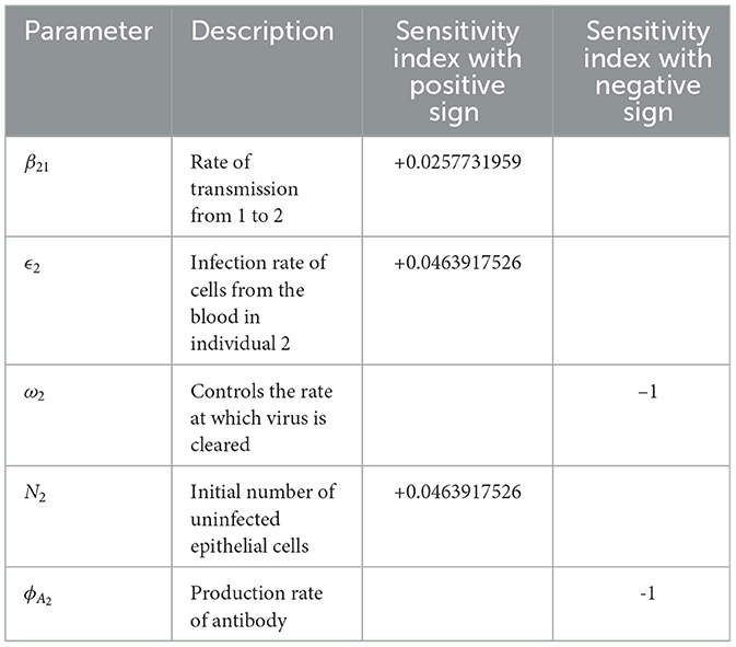
Table 4. Sensitivity indices of model reproduction number ${\mathcal{R}}_0$ to parameters for model system (Equations 1–8), evaluated at the parameter values presented in Table 3.

4.1.2 Global sensitivity analysis

This section presents the analysis of sensitivity for the FMDV transmission indicators obtained from the multiscale model to the model parameters. The transmission indicator we consider is the basic reproductive number, ${\mathcal{R}}_0$ that generally describes the dynamics for a disease at the beginning of an infection. For any particular epidemic model that illustrates the disease dynamics within a particular population, a sensitivity analysis study is important to perform since it enables us to establish model parameters which can be marked for control, elimination as well as eradication of disease. Therefore, the analysis of sensitivity of the FMDV metric ${\mathcal{R}}_0$, in relation to the variation of FMD multiscale model parameters is carried out by implementing Latin Hypercube Sampling and Partial Rank Correlation Coefficients (PRCCs). In order to explore the influence of each model parameter on the basic reproduction number, ${\mathcal{R}}_0$ we performed 1,000 simulations per run. The results of sensitivity of ${\mathcal{R}}_0$ to the model parameters are presented by the Tornado plot in Figure 2.

Figure 2

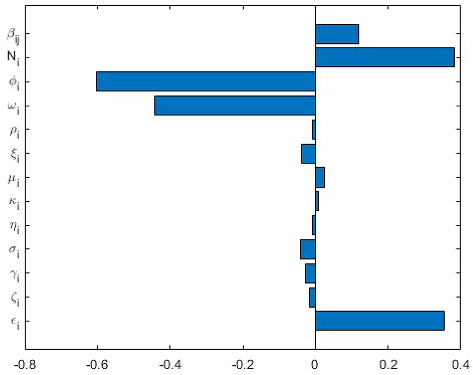
Figure 2. Tornado plot of partial rank correlation coefficients (PRCCs) of the multiscale model parameters that impact the FMDV transmission indicator ${\mathcal{R}}_0$.

According to the sensitivity analysis results of ${\mathcal{R}}_0$ to the multiscale model system's (Equations 1–8) parameters obtained in Figure 2, we deduce these outcomes:

(a) The multiscale model system's (Equations 1–8) parameters have both positive PRCCs and negative PRCCs. This implies that parameters with positive PRCCs will increase the value of ${\mathcal{R}}_0$ as they are increased, where as parameters with negative PRCCs will decrease the value for ${\mathcal{R}}_0$ as they are increased. For example, an increase in a parameter such as rate of infection of cells from the blood, ϵ_i at the within-host level will consequently increase the value of ${\mathcal{R}}_0$, and also increasing a parameter such as rate at which virus is cleared, ω_i leads to decrease in ${\mathcal{R}}_0$.

(b) The FMDV transmission metric ${\mathcal{R}}_0$ is extremely sensitive to five of the disease parameters of the multiscale model system (Equations 1–8), ( β_ij, N_i, ϕ_i, ω_i, ϵ_i). We note that ${\mathcal{R}}_0$ indicates spread of FMDV during the beginning of the outbreak. The following conclusions regarding sensitivity of ${\mathcal{R}}_0$ to the FMDV multiscale model system's (Equations 1–8) parameters can be established.

(i) Since ${\mathcal{R}}_0$ is significantly sensitive to (β_ij, N_i, ϕ_i, ω_i, ϵ_i), this implies that caution must be applied on the accuracy of these five FMDV multiscale model system's (Equations 1–8) parameters during the collection of data if the effectiveness and usefulness of the FMDV multiscale model system (Equations 1–8) is to be intensified.

(ii) In view of the fact that ${\mathcal{R}}_0$ is responsive to the transmission rate between the cattle, β_ij (the between-host level parameter) it implies that FMD interventions such as quarantines would be more effective to control the spread of FMD infection at the beginning of the outbreak.

(iii) Since ${\mathcal{R}}_0$ is significantly sensitive to the initial susceptible epithelial cells, N_i (the within-host level parameter) and the rate of infection of cells from the blood, ϵ_i this implies that FMD interventions such as vaccination (which reduces susceptible epithelial cells within the cattle) would be more effective to control the spread of FMD infection at the beginning of outbreak.

(iv) Since ${\mathcal{R}}_0$ is significantly sensitive to the rate of production of antibodies, ϕ_Ai and rate at which FMDV virus is cleared, ω_i this implies that FMD interventions such as vaccination (which increases the rate of antibody production and clearance of FMDV virus) would be more effective to control the spread of FMD infection at the beginning of outbreak.

4.2 Numerical simulations of the multiscale model of FMD transmission dynamics

This section enables us to implement numerical simulations to substantiate some outcomes obtained from the sensitivity analysis for ${\mathcal{R}}_0$ and analytical results of the multiscale model. Applying the multiscale model parameter values obtained from Table 2 we carried out the numerical simulations. We demonstrate the impact of five FMD transmission parameters (β_ij, N_i, ϕ_i, ω_i, ϵ_i) on the multiscale model variables V_i, F_i, U_i, P_i, I_i, A_i, C_i, J_i. These parameters were only selected because they are significantly sensitive to ${\mathcal{R}}_0$.

4.2.1 Influence of within-host scale parameters of the FMD multiscale model dynamics

In this section, we demonstrate by implementing numerical simulations the impact of within-host scale parameters

Figure 3 represents the graphs of numerical results of model system (Equations 1–8) demonstrating the progression in time of (a) concentration of virions in the blood for individual 1, V₁, (b) concentration of virions in the blood for individual 2, V₂, (c) infected cells for individual 1, F₁, (d) infected cells for individual 2, F₂ for variant values of infection rate of cells from the blood for individual 1, ϵ₁:ϵ₁ = 0.003, ϵ₁ = 0.03 and ϵ₁ = 0.3. From these results we can see that as the rate of infection of cells from the blood for individual 1, ϵ₁ increases, there is significant increase in the concentration of virions in the blood for individual 1, concentration of virions in the blood for individual 2, infected cells for individual 1, infected cells for individual 2. These results reflect that interventions such as vaccination of cattle will reduce the rate of infection of cells from the blood leading to a reduced risk of transmission of FMD for the individual in the community.

Figure 3

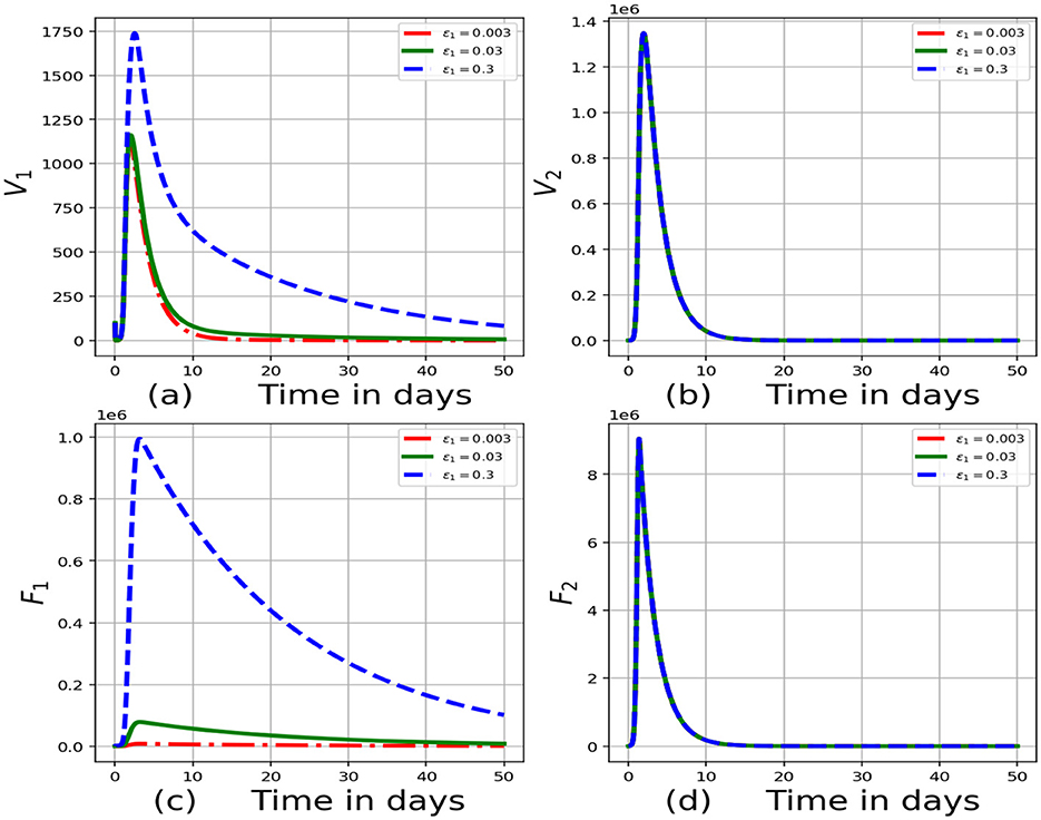
Figure 3. Graphs of numerical results of the model system (Equations 1–8) demonstrating the advancement with time of (a) concentration of virions in the blood for individual 1, V₁, (b) concentration of virions in the blood for individual 2, V₂, (c) infected cells for individual 1, F₁, (d) infected cells for individual 2, F₂ for variant values of infection rate of cells from the blood for individual 1, ϵ₁:ϵ₁ = 0.003, ϵ₁ = 0.03 and ϵ₁ = 0.3.

Figure 4 demonstrates the impact of variation of rate at which virus is cleared, ω₁:ω₁ = 0.006, ω₁ = 0.06 and ω₁ = 0.6 on the within-host scale variables V_i, F_i, U_i, P_i, I_i, A_i, C_i, J_i. The outcomes demonstrate that a decrease in ω is related to an increment in the within-cattle scale variables (V_i, F_i, I_i, C_i, J_i). An increment in the within-cattle scale variables like V_i and F_i implies that there is an increase in FMDV shedding into the environment and an increase in the strength of transmission of FMDV, β, throughout the cattle population. The within-host scale variables I_i, C_i, A_i represent the early immune response which intensifies as rate at which virus is cleared decreases. These results reflect that interventions such as vaccination of cattle will increase the clearance rate of virus leading to a reduced risk of transmission of FMD for each individual in the community. This can be justified by Equation 36, which shows that when the clearance rate of virus is increased, the value of R₀ decreased.

Figure 4

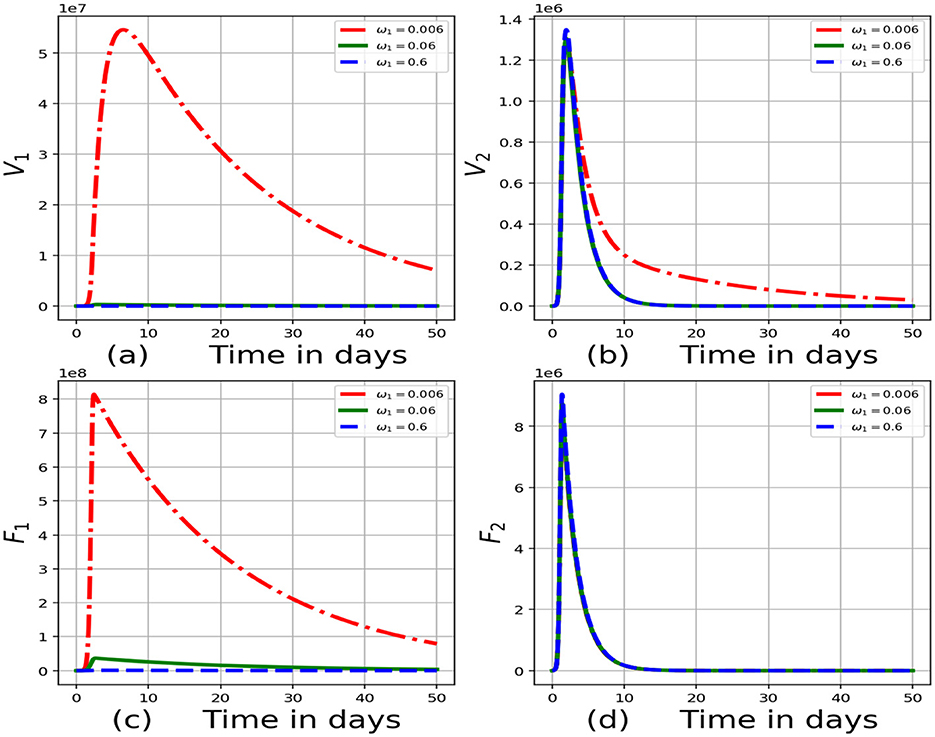
Figure 4. Graphs of numerical results of the model system (Equations 1–8) demonstrating the advancement with time of (a) concentration of virions in the blood for individual 1, V₁, (b) concentration of virions in the blood for individual 2, V₂, (c) infected cells for individual 1, F₁, (d) infected cells for individual 2, F₂ for variant values of rate at which virus is cleared for individual 1, ω₁:ω₁ = 0.006, ω₁ = 0.06 and ω₁ = 0.6.

4.2.2 Influence of between-host scale parameters of the FMD multiscale model dynamics

Figure 5 represents the graphs of numerical results of the model system (Equations 1–8) demonstrating the advancement with time of all model variables for variant values of rate of transmission of virus from individual 2 to individual 1, β₂₁:β₂₁ = 0.003, β₂₁ = 0.03 and β₂₁ = 0.3. Results indicate that as the rate of transmission of virus from individual 2 to individual 1 increases, there is an increase in the within-cattle scale variables such as V₁ and F₁. Intervention strategies such as quarantines would be more effective in reducing the rate of transmission. This can be justified by Equation 36, which shows that when the rate of transmission of virus from individual 2 to individual 1 is decreased, the value of R₀ decreased.

Figure 5

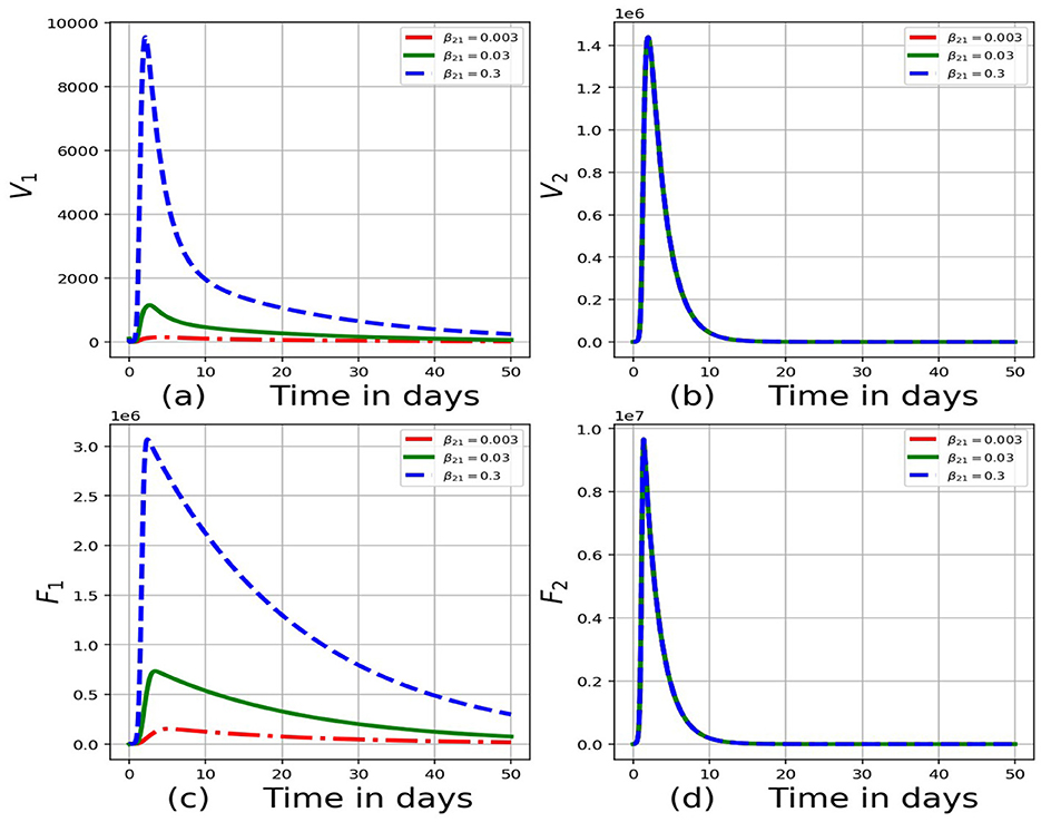
Figure 5. Graphs of numerical results of the model system (Equations 1–8) demonstrating the advancement with time of (a) concentration of virions in the blood for individual 1, V₁, (b) concentration of virions in the blood for individual 2, V₂, (c) infected cells for individual 1, F₁, (d) infected cells for individual 2, F₂ for variant values of rate of transmission of virus from individual 2 to individual 1, β₂₁:β₂₁ = 0.003, β₂₁ = 0.03 and β₂₁ = 0.3.

Figure 6 represents a network visualization based on the degree distribution of 50 cattle as a result of data generated by stochastic simulation approach (source code: Appendix B). The nodes represent cattle in the network and links represent the possible transmissions. The nodes with the highest node degree (number of connections) may indicate the presence of hubs or super-spreaders. Therefore, if hubs exist, targeted interventions such as isolation or vaccination (which reduces susceptible epithelial cells within the cattle) would have a positive impact in controlling the spread of FMD in cattle. Furthermore, the network has a uniform or Poisson distribution of node degree which implies there is lack of clustering and degree correlation that is observed in other complex networks.

Figure 6

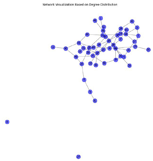
Figure 6. The network visualization based on the degree distribution of 50 cattle.

Figure 7 represents a degree distribution histogram which visualizes how node degrees (number of connections) are distributed in a network. Since the histogram is not heavy-tailed, this does not indicate the existence of super-spreaders or hubs. Therefore, targeted intervention such as vaccination to vulnerable groups would impact positively in controlling the spread of FMD in the cattle population.

Figure 7

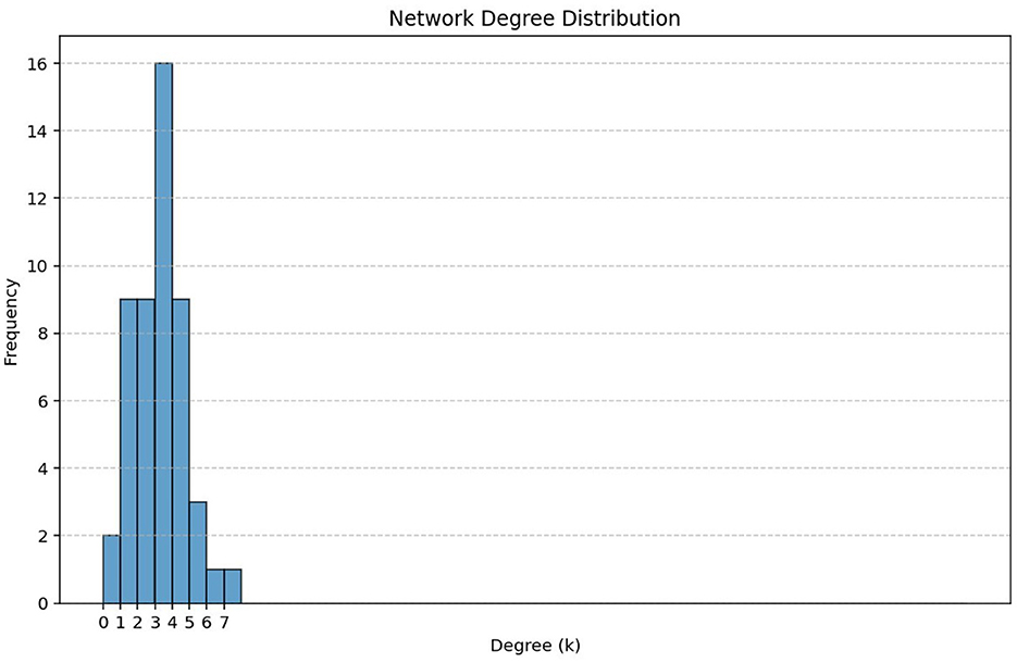
Figure 7. The network degree distribution in the cattle population.

Figure 8 shows scatterplots visualizing relationships between various pairs of variables in the FMD multiscale model. For example, there is a strong negative correlation between Infected cells and Interferons. This shows the impact of immune response since the infected cells decrease as the interferons are activated. Furthermore, there is a negative correlation between Infected cells and Virions. This is because as the infected cells burst, their population is reduced resulting in increased amounts of virions in the blood. Therefore, intervention strategies such as vaccination would help to combat the spread of FMD in cattle.

Figure 8

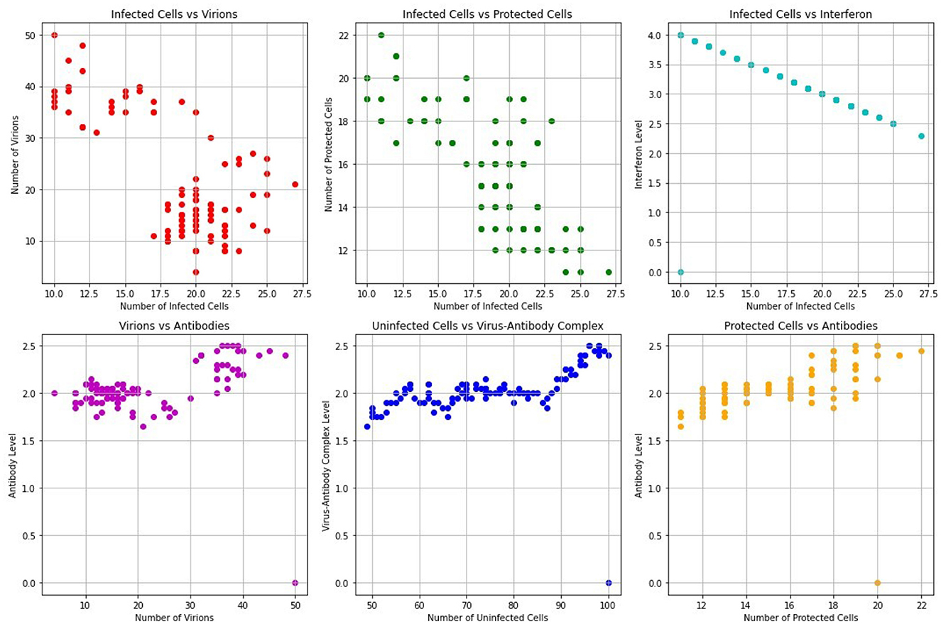
Figure 8. The relationships between various pairs of variables.

Figure 9 consist of the graphs (in black) representing the means of the dynamics for 50 cattle and the graphs (in blue) representing the dynamics of each individual animal for Infected cells (F_i), Virions in blood, (V_i), Interferon, (I_i) and Virus-Antibody Complexes, (C_i). The graphs indicate heterogeneity in: host susceptibility to infection, the ability of hosts to transmit pathogen to other hosts and host immune response for the 50 cattle (source code: Appendix A). Therefore, targeted interventions such as vaccination and isolation of the vulnerable group would have more impact in combating the spread of FMD.

Figure 9

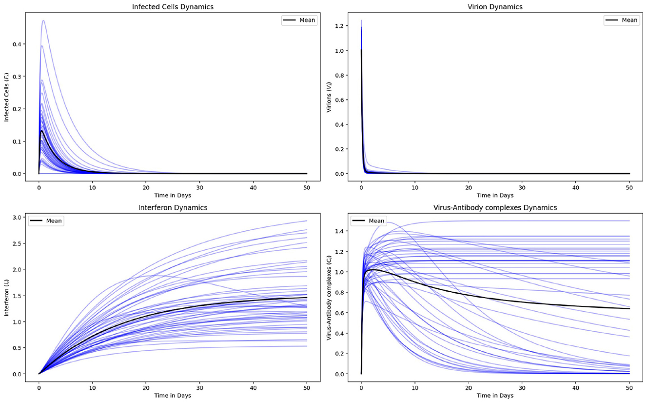
Figure 9. The graphs (in black) represent the means of the dynamics for 50 cattle and the graphs (in blue) represent the dynamics of each individual animal for Infected cells (F_i), Virions in blood, (V_i), Interferon, (I_i) and Virus-Antibody Complexes, (C_i).

Figure 10 shows a correlation heatmap of model variables (F_i, V_i, P_i, U_i). Results show that there is a negative correlation between Infected cells and Virions. This is because as the infected cells burst, their population is reduced resulting in increased amounts of virions in the blood. Furthermore, there is a positive correlation between Protected cells and Uninfected cells. This is because as the population of protected cells increases, the population of uninfected cells will also increase. Therefore, intervention strategies such as vaccination (which reduces susceptible epithelial cells within the cattle) would help to combat the spread of FMD.

Figure 10

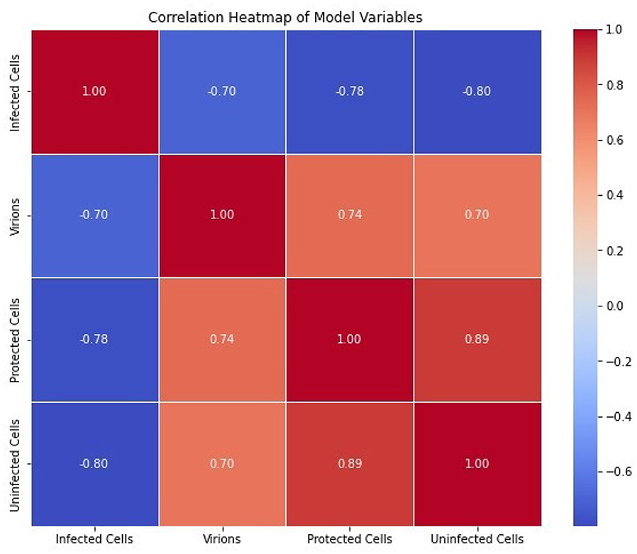
Figure 10. The correlation of different pairs of model variables (F_i, V_i, P_i, U_i).

Figure 11 shows the contact matrix with various transmission probabilities. The darkest color represents the highest transmission probability and lightest color represents the lowest transmission probability. Therefore, targeted intervention strategies such as vaccination or quarantine of vulnerable groups would be more effective in combating the spread of FMD.

Figure 11

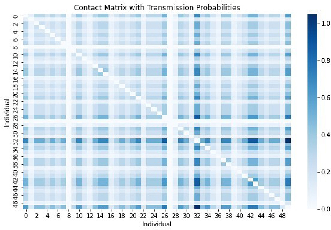
Figure 11. The contact matrix with various transmission probabilities. The darkest color represents the highest transmission probability and lightest color represents the lowest transmission probability.

4.3 Mean-field approximation (homogeneous mixing) of multiscale model

We now consider the mean-field approximation, a simplification used to reduce complex interactions into an averaged effect. This can be compared with the multiscale model system (Equations 1–8) to explore similarities or deviations.

$\begin{array}{ll}\frac{dV}{dt}=<k>\zeta F-{\varphi }_A\omega V,& (96)\end{array}$

$\begin{array}{ll}\frac{dF}{dt}=ϵUV-<k>\zeta F,& (97)\end{array}$

$\begin{array}{ll}\frac{dU}{dt}=-\kappa U\left(I-\frac{\mu }{\xi }\right),& (98)\end{array}$

$\begin{array}{ll}\frac{dP}{dt}=\kappa U\left(I-\frac{\mu }{\xi }\right),& (99)\end{array}$

$\begin{array}{ll}\frac{dI}{dt}=\mu -\xi I+{\varphi }_U(U)\eta C,& (100)\end{array}$

$\begin{array}{ll}\frac{dA}{dt}={\varphi }_V(V,J){\varphi }_A,& (101)\end{array}$

$\begin{array}{ll}\frac{dC}{dt}={\varphi }_A\omega (V+J)-\sigma C,& (102)\end{array}$

$\begin{array}{ll}\frac{dJ}{dt}=\gamma \zeta F-{\varphi }_A\omega J& (103)\end{array}$

where < k > is the average degree (number of contacts) in the network. The model variables and parameters in model system (Equations 1–8) have been simplified from the model variables and parameters in model system (Equations 1–8). The numerical simulation of the model system (Equations 1–8) is given in Figure 12.

Figure 12

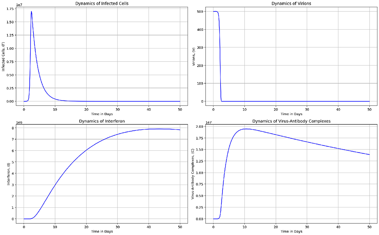
Figure 12. The graphs represent the dynamics of Infected cells, (F), Virions in blood, (V), Interferon, (I), and Virus-Antibody Complexes, (C).

Figure 12 consists of the graphs representing the dynamics of Infected cells, (F), Virions in blood, (V), Interferon, (I), and Virus-Antibody Complexes, (C). Results indicate that the graphs (in black) for model system (Equations 1–8) representing the means of the dynamics for 50 cattle in Figure 9 do not deviate from the mean-field predictions in model system (Equations 1–8). It is also important to highlight that multiscale models such as coupled multiscale models and nested multiscale models are examples of mean-field approximations which require more detailed comparison in future studies.

4.4 Effects of stochasticity on the model

In this section we introduce a white noise (dW_Q/dt) (that is, W(t) is a Brownian motion), where Q = {V_i, F_i, U_i, P_i, I_i, A_i, C_i, J_i}, into multiscale model system (Equations 1–8) which becomes

$\begin{array}{ll}\{\begin{array}{l}d{V}_i=\left[{\zeta }_i{F}_i-{\varphi }_{A_i}{\omega }_i{V}_i+{\displaystyle \underset{i\ne j}{\sum ^n}}{\beta }_{ij}{V}_j\right]dt+{\sigma }_{V_i}{V}_{i}d{W}_V(t),\\ d{F}_i=\left[{ϵ}_i{U}_i{V}_i-{\zeta }_i{F}_i\right]dt+{\sigma }_{F_i}{F}_{i}d{W}_F(t),\\ d{U}_i=\left[-{\kappa }_i{U}_i\left(I_i-\frac{{\mu }_i}{{\xi }_i}\right)\right]dt+{\sigma }_{U_i}{U}_{i}d{W}_U(t),\\ d{P}_i=\left[{\kappa }_i{U}_i\left(I_i-\frac{{\mu }_i}{{\xi }_i}\right)\right]dt+{\sigma }_{P_i}{P}_{i}d{W}_P(t),\\ d{I}_i=\left[{\mu }_i-{\xi }_i{I}_i+{\varphi }_{U_i}(U){\eta }_i{C}_i\right]dt+{\sigma }_{I_i}{I}_{i}d{W}_I(t),\\ d{A}_i=\left[{\varphi }_{V_i}(V,J){\varphi }_{A_i}\right]dt+{\sigma }_{A_i}{A}_{i}d{W}_A(t),\\ d{C}_i=\left[{\varphi }_{A_i}{\omega }_i(V_i+J_i)-{\sigma }_i{C}_i\right]dt+{\sigma }_{C_i}{C}_{i}d{W}_C(t),\\ d{J}_i=\left[{\gamma }_i{\zeta }_i{F}_i-{\varphi }_{A_i}{\omega }_i{J}_i\right]dt+{\sigma }_{J_i}{J}_{i}d{W}_J(t)\end{array}& (104)\end{array}$

We set W(t) = W_V(t), W_F(t), W_U(t), W_P(t), W_I(t), W_A(t), W_C(t), W_J(t) an 8-dimensional Wiener process that is defined on this probability space. Further, the constants σ_Vi, σ_Fi, σ_Ui, σ_Pi, σ_Ii, σ_Ai, σ_Ci, σ_Ji and non-negative and describe the intensities of the stochastic pertubations. Let us assume that the components of the 1-dimensional Wiener process W_i are mutually independent. It can be shown that the SDE model (Equation 104) has at least a unique global solution in order for the model to have meaning and also that the solution will always remain positive whenever the initial conditions are positive. Let us consider the following theorem.

Proposition 1. For Equation 104 and any initial value in ${ℝ}_{+}^8$, there is a unique solutionL = (V_i, F_i, U_i, P_i, I_i, A_i, C_i, J_i) where i = 1, ..., n of the system (Equation 104) for t ≥ 0 which will remain in ${ℝ}_{+}^8$ with probability one.

Figure 13 demonstrates the graphs of numerical results of infectious virions in blood in the 1st individual, V₁ of the multiscale SDE model system (Equation 104) with the ODE multiscale model system (Equations 1–8) solutions. For the Stochastic differential equation the intensity of the stochastic pertubations σ = 0.3. The solution for the stochastic multiscale model is obtained using the Milsten method.

Figure 13

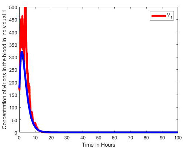
Figure 13. Graphs of numerical results of infectious virions in blood in the 1st individual, V₁ of the multiscale SDE model system (Equation 104) with the ODE multiscale model system (Equations 1–8) solutions. For the Stochastic differential equation the intensity of the stochastic pertubations σ = 0.3.

Figure 14 demonstrates the graphs of numerical results of the infected cells in the 1st individual, F₁ of the multiscale SDE model system (Equation 104) with the ODE multiscale model system (Equations 1–8) solutions. For the Stochastic differential equation the intensity of the stochastic pertubations σ = 0.3. The solution for the stochastic multiscale model is obtained using the Milsten method.

Figure 14

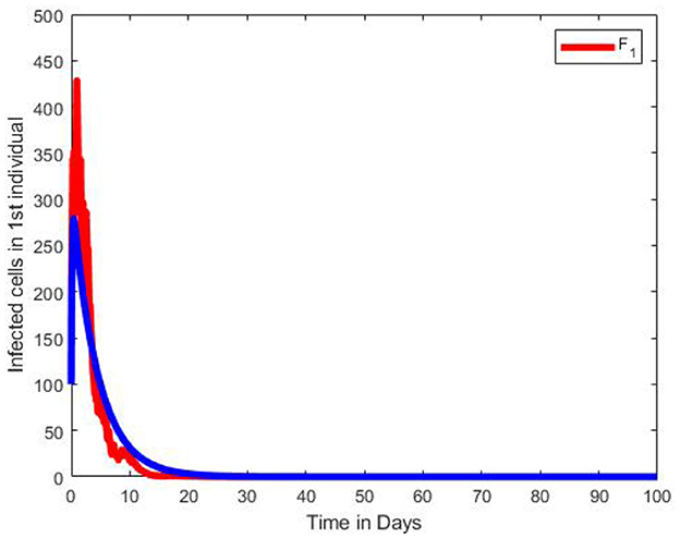
Figure 14. Graphs of numerical results of the infected cells in the 1st individual, F₁ of the multiscale SDE model system (Equation 104) with the ODE multiscale model system (Equations 1–8) solutions. For the Stochastic differential equation the intensity of the stochastic pertubations σ = 0.3.

5 Discussion and conclusions

The primary contribution of this study to scientific understanding is the development of an individual-based multiscale network model, grounded in the replication-transmission relativity theory, which integrates the within-host and between-host dynamics of infectious disease systems. It incorporates the pathogen replication cycle at the within-host level, utilizing Foot-and-mouth disease (FMD) in cattle as a case study. A key characteristic of individual-based multiscale network models is the variation in (i) host susceptibility to infection, (ii) the capability of hosts to transmit the pathogen to others, (iii) the immune response of hosts, and (iv) host behavior. Based on the sensitivity analysis, it is evident that the reproduction number is influenced by certain parameters, including the transmission rate among cattle (a between-host parameter), the initial count of susceptible epithelial cells, the rate at which cells become infected from the blood, the antibody production rate, and the rate at which the FMD virus is eliminated (within-host parameters). This suggests that interventions for FMD, such as vaccination (which activates the immune response to eliminate the FMD virus and thus lowers replication), along with bio-security measures like disinfecting vehicles, equipment, and footwear, as well as isolating new animals prior to their introduction, would be more effective in curbing the spread of FMD at the onset of an outbreak. Numerical simulations were conducted to demonstrate the influence of model parameters designated for controlling, eliminating, and eradicating FMD. The results of the simulations suggest that non-pharmacological strategies such as disinfection, quarantine, wildlife management, surveillance, and early detection can be utilized to reduce the transmission rate of FMDV within the cattle population. Additionally, the analysis of the network degree distribution indicates the absence of hubs due to lack of a heavy tail on the histogram. It is also important to highlight that the network has a uniform or Poisson distribution of node degree which implies lack of clustering and degree correlation that is observed in other complex networks such as scale-free and small-world.

This research offers valuable insights to mathematical modelers regarding the integration of varying scales across all levels of biological hierarchy. The primary focus of this study was the development and analysis of an individual-based multiscale network model. However, future research will incorporate more realistic complex networks such as scale-free networks characterized by a few highly connected nodes (hubs) and many nodes with few connections. These hubs (super-spreaders) might be responsible for a disproportionately large number of disease transmissions.

Data availability statement

The raw data supporting the conclusions of this article will be made available by the authors, without undue reservation.

Author contributions

BM: Conceptualization, Methodology, Visualization, Writing – original draft. WG: Conceptualization, Supervision, Writing – review & editing. DM: Methodology, Writing – review & editing.

Funding

The author(s) declare that no financial support was received for the research and/or publication of this article.

Conflict of interest

The authors declare that the research was conducted in the absence of any commercial or financial relationships that could be construed as a potential conflict of interest.

Generative AI statement

The author(s) declare that no Gen AI was used in the creation of this manuscript.

Publisher's note

All claims expressed in this article are solely those of the authors and do not necessarily represent those of their affiliated organizations, or those of the publisher, the editors and the reviewers. Any product that may be evaluated in this article, or claim that may be made by its manufacturer, is not guaranteed or endorsed by the publisher.

Supplementary material

The Supplementary Material for this article can be found online at: https://www.frontiersin.org/articles/10.3389/fams.2025.1608265/full#supplementary-material

References

1. Garira W, Mathebula D, Netshikweta R. A mathematical modelling framework for linked within-host and between-host dynamics for infections with free-living pathogens in the environment. Math Biosci. (2014) 256:58–78. doi: 10.1016/j.mbs.2014.08.004

PubMed Abstract | Crossref Full Text | Google Scholar

2. Garira W, Chirove F. A general method for multiscale modelling of vector-borne disease systems. Interface Focus. (2020) 10:20190047. doi: 10.1098/rsfs.2019.0047

PubMed Abstract | Crossref Full Text | Google Scholar

3. Garira W. A complete categorization of multiscale models of infectious disease systems. J Biol Dyn. (2017) 11:378–435. doi: 10.1080/17513758.2017.1367849

PubMed Abstract | Crossref Full Text | Google Scholar

4. Garira W. A primer on multiscale modelling of infectious disease systems. Infect Dis Model. (2018) 3:176–91. doi: 10.1016/j.idm.2018.09.005

PubMed Abstract | Crossref Full Text | Google Scholar

5. Garira W. The research and development process for multiscale models of infectious disease systems. PLoS Comput Biol. (2020) 16:e1007734. doi: 10.1371/journal.pcbi.1007734

PubMed Abstract | Crossref Full Text | Google Scholar

6. Garira W. The replication-transmission relativity theory for multiscale modelling of infectious disease systems. Sci Rep. (2019) 9:16353. doi: 10.1038/s41598-019-52820-3

PubMed Abstract | Crossref Full Text | Google Scholar

7. Keeling MJ, Eames KTD. Networks and epidemic models. J R Soc Interface. (2005) 2:295–307. doi: 10.1098/rsif.2005.0051

PubMed Abstract | Crossref Full Text | Google Scholar

8. Donaldson AI, Alexandersen S. Predicting the spread of foot and mouth disease by airborne virus. Rev Sci Tech. (2002) 21:569–78. doi: 10.20506/rst.21.3.1362

PubMed Abstract | Crossref Full Text | Google Scholar

9. Woolhouse MEJ. Foot-and-mouth disease in the UK: What should we do next time? J Appl Microbiol. (2003) 94:126–30. doi: 10.1046/j.1365-2672.94.s1.15.x

PubMed Abstract | Crossref Full Text | Google Scholar

10. Thompson D, Muriel P, Russell D, Osborne P, Bromley A, Rowland M, et al. Economic costs of the foot and mouth disease outbreak in the united kingdom in 2001. Rev Sci Tech. (2002) 21:675–87. doi: 10.20506/rst.21.3.1353

PubMed Abstract | Crossref Full Text | Google Scholar

11. Sinkala Y, Simuunza M, Muma JB, Pfeiffe DU, Kasanga CJ, Mweene A, et al. Foot and mouth disease in Zambia: Spatial and temporal distributions of outbreaks, assessment of clusters and implications for control. Onderstepoort J Vet Res. (2014) 81:1–6. doi: 10.4102/ojvr.v81i2.741

PubMed Abstract | Crossref Full Text | Google Scholar

12. Ringa N, Bauch CT. Impacts of constrained culling and vaccination on control of foot and mouth disease in near-endemic settings: a pair approximation model. Epidemics. (2014) 9:18–30. doi: 10.1016/j.epidem.2014.09.008

PubMed Abstract | Crossref Full Text | Google Scholar

13. Roche SE, Garner MG, Sanson RL, Cook C, Birch C, Backer JA, et al. Evaluating vaccination strategies to control foot-and-mouth disease: a model comparison study. Epidemiol Infect. (2015) 143:1256–75. doi: 10.1017/S0950268814001927

PubMed Abstract | Crossref Full Text | Google Scholar

14. Rawdon TG, Garner MG, Sanson RL, Stevenson MA, Cook C, Birch C, et al. Evaluating vaccination strategies to control foot-and-mouth disease: a country comparison study. Epidemiol Infect. (2018) 146:1138–50. doi: 10.1017/S0950268818001243

PubMed Abstract | Crossref Full Text | Google Scholar

15. Eschbaumer M, Stenfeldt C, Rekant SI, Pacheco JM, Hartwig EJ, Smoliga GR, et al. Systemic immune response and virus persistence after foot-and-mouth disease virus infection of naive cattle and cattle vaccinated with a homologous adenovirus-vectored vaccine. BMC Vet Res. (2016) 12:205. doi: 10.1186/s12917-016-0838-x

PubMed Abstract | Crossref Full Text | Google Scholar

16. Bradhurst RA, Roche SE, East IJ, Kwan P, Garner MG. A hybrid modeling approach to simulating foot-and-mouth disease outbreaks in Australian livestock. Front Environ Sci. (2015) 3:17. doi: 10.3389/fenvs.2015.00017

Crossref Full Text | Google Scholar

17. Kao RR, Green DM, Johnson J, Kiss IZ. Disease dynamics over very different time-scales: foot-and-mouth disease and scrapie on the network of livestock movements in the UK. J R Soc Interface. (2007) 4:907–16. doi: 10.1098/rsif.2007.1129

PubMed Abstract | Crossref Full Text | Google Scholar

18. Kostova-Vassilevska T. On the Use of Models to Assess Foot-and-Mouth Disease Transmission and Control. Technical report. Livermore, CA: Lawrence Livermore National Lab (2004). doi: 10.2172/15014467

Crossref Full Text | Google Scholar

19. Howey R, Quan M, Savill NJ, Matthews L, Alexandersen S, Woolhouse M, et al. Effect of the initial dose of foot-and-mouth disease virus on the early viral dynamics within pigs. J R Soc Interface. (2009) 6:835–47. doi: 10.1098/rsif.2008.0434

PubMed Abstract | Crossref Full Text | Google Scholar

20. Howey R, Bankowski B, Juleff N, Savill NJ, Gibson D, Fazakerley J, et al. Modelling the within-host dynamics of the foot-and-mouth disease virus in cattle. Epidemics. (2012) 4:93–103. doi: 10.1016/j.epidem.2012.04.001

PubMed Abstract | Crossref Full Text | Google Scholar

21. Tuckwell HC, Toubiana L, Vibert J-F. Spatial epidemic network models with viral dynamics. Phys Rev E. (1998) 57:2163. doi: 10.1103/PhysRevE.57.2163

Crossref Full Text | Google Scholar

22. Castillo-Chavez C, Feng Z, Huang W. On the computation of R_0 and its role in global stability. In:Castillo-Chavez C, Blower S, van den Driessche P, Kirschner D, , editors. Mathematical Approaches for Emerging and Re-Emerging Infectious Diseases Part 1: An Introduction to Models, Methods and Theory. The IMA Volumes in Mathematics and Its Applications, Vol. 125. Berlin: Springer-Verlag (2002). p. 229–50. doi: 10.1007/978-1-4613-0065-6

Crossref Full Text | Google Scholar

23. Diekmann O, Heesterbeek JAP, Metz JAJ. On the definition and the computation of the basic reproduction ratio r 0 in models for infectious diseases in heterogeneous populations. J Math Biol. (1990) 28:365–82. doi: 10.1007/BF00178324

PubMed Abstract | Crossref Full Text | Google Scholar

24. Van den Driessche P, Watmough J. Reproduction numbers and sub-threshold endemic equilibria for compartmental models of disease transmission. Math Biosci. (2002) 180:29–48. doi: 10.1016/S0025-5564(02)00108-6

PubMed Abstract | Crossref Full Text | Google Scholar

25. Chitnis N, Hyman JM, Cushing JM. Determining important parameters in the spread of malaria through the sensitivity analysis of a mathematical model. Bull Math Biol. (2008) 70:1272. doi: 10.1007/s11538-008-9299-0

PubMed Abstract | Crossref Full Text | Google Scholar

26. Njagarah JBH, Nyabadza F. Modeling the impact of rehabilitation, amelioration and relapse on the prevalence of drug epidemics. J Biol Syst. (2013) 21:1350001. doi: 10.1142/S0218339013500010

PubMed Abstract | Crossref Full Text | Google Scholar