Insights into pre-reversal paleosecular variation from stochastic models

Introduction

The Earth's magnetic field is one of the most representative characteristics of our planet. There is a widespread consent that the main geomagnetic field is of internal origin and is created and maintained by a dynamo mechanism in the molten outer core of the Earth (Moffatt, 1978). The external sources (ionosphere, magnetosphere, ring currents) have noticeable contributions although smaller than the contributions from internal sources. However these outer sources remain important to explain some features of the temporal changes of the geomagnetic field.

The field observed at the Earth's surface is mainly dipolar, at least for the last five Myr (Heimpel and Evans, 2013) and is subject to temporal changes in a wide range of time scales, from 10⁻³ s to 10⁸ years. The time variations with time scales shorter than several months are considered to have an external origin, while the time variation with a longer time scale are mainly of internal origin. The time variation with time scale from months to thousands of years is termed secular variation (SV) contains a small contribution from external origin, especially those variations of time scales of months to 10 years. Variations with longer time scale, namely geomagnetic field reversals or excursions, are properly due to internal sources (Merrill and Mcfadden, 1999).

A reversal is a complete flip of the polarity of the magnetic dipolar moment of the geomagnetic field (Krijgsman and Kent, 2004). The paleomagnetic data show that the Earth's magnetic field has experienced hundreds of polarity reversals during the planet's history. These reversals occurred at irregular intervals (Jacobs, 1994; Merrill et al., 1996) with durations of constant polarity lasting from 40 kyr to 40 Myr. The geomagnetic field reversals sequence of the last 160 Myr shows that the distribution of the length of the intervals between two consecutive reversals fits a lognormal distribution (Ryan and Sarson, 2007). Other authors derive different conclusions showing that the distribution of the chrons between reversals fits other statistical distributions like gamma distribution (Naidu, 1971) and Poisson distribution (Constable and Parker, 1988). Actually the picture is more complex because there are registered excursions as well that are considered to be two consecutive reversals bracketing an aborted polarity interval (Valet et al., 2008).

Despite of the increasing data which enhance our understanding on SV, especially abrupt changes such as jerks (Duka et al., 2012), there is yet unknown a physical mechanism that can fully and satisfactorily describe these features of the geomagnetic field. Apparently the short term changes (SV) and the reversals have different statistical behavior this being evidence that these features of the geomagnetic field are controlled by different physical mechanisms. However, now it is almost accepted that reversals are natural outgrowths of the SV (Gubbins, 1999; Biggin et al., 2008; Lhuillier and Gilder, 2013), and that these events occur during a persistent period of low intensity of dipolar magnetic field (Guyodo and Valet, 1999).

Measurements of the Earth magnetic field show that in the last centuries the dipolar moment has decreased and such decreasing is lasting for longer periods as given by different SV models like CALS7K.2, CALSK.10b, or SHA.DIF.14K (Korte and Constable, 2005; Genevey et al., 2008; Knudsen et al., 2008; Pavon-Carasco et al., 2014). There are authors that argue although the field intensity is rapidly decreasing, a reversal in the near future may be improbable (Cox, 1969). Others speculate the opposite (De Santis and Qamili, 2015).

Much of the magnetic field variations are thought to have a stochastic nature and almost all kinds of different models: phenomenological, experimental, or numerical (Petrelis et al., 2009) of the temporal changes of the magnetic field are based on stochastic processes, most of them treating the geomagnetic field as a dynamical system. On the other hand, some authors (Barraclough and De Santis, 1997) suggest that the geomagnetic field has a chaotic behavior becoming unpredictable after a time period of several years.

Numerical simulations are a very helpful tool to study the statistical behavior of the geomagnetic field, to provide some insights in its dynamics and probably to predict near future changes. The numerical models span from models based on magneto-hydrodynamics (MHD) partial differential equations (Rüdiger and Hollerbach, 2004; Christensen and Wicht, 2007) to “toy” models like the “domino” model (Nakamichi et al., 2011; Mori et al., 2013; Duka et al., 2015) or Rikitake two-disk dynamo (Hoshi and Kono, 1988). The time series obtained by numerically simulating various MHD models show that geomagnetic field reversals occur by imposing different conditions and different parameter values on the 3D dynamo equations (Glatzmaier and Roberts, 1995, 1997; Glatzmaier et al., 1999). Some succeeded to reproduce some features of the SV (Schmitt et al., 2001; Christensen and Olson, 2003).

The complexity of the MHD equations requires powerful computational resources that often are inaccessible, whereas “toy” models can be simulated easily with a PC. Despite their simplicity, “toy” models seem to reproduce quite accurately many features of the geomagnetic field temporal variations. One of these models, the “domino” model, appears with several versions, but two of them are of particular interest: the Short-range Coupled Spins (SCS) model (Mori et al., 2013) and the Long-range Coupled Spins (LCS) model (Nakamichi et al., 2011; Duka et al., 2015). Another model is the Rikitake model. Many extended versions can be found in the literature, but in this paper we will take in consideration the inhomogeneous Lebovitz (IL) model (Shimizu and Honkura, 1985). According to these authors, the IL model is the most appropriate in modeling the geomagnetic field reversals. In the present work we extend their study by controlling their result and analysing how efficient the IL model is in reproducing the SV behavior of the Earth magnetic field.

In the dynamical equations of the SCS and LCS models, there is an important random term (see Section Statistical Models below), which makes the name stochastic model quite accurate. As a consequence, the magnetisation time series generated by these models show random polarity flips (Duka et al., 2015). For the IL model, the random behavior is the result of the specific interactions among disks.

Similarly to Duka et al. (2015), we study the parameter space of the models although our study is not conclusive. We aim to find that set of parameter values (for each model) for which the statistical behavior of the time series generated by simulating the models is similar to the behavior of the SHA.DIF.14K time series. After we found these sets of parameter values, we extended the time series covering the near future. We do not pretend to give a prediction of the future behavior of the geomagnetic field because it has chaotic nature (Barraclough and De Santis, 1997; De Santis et al., 2011). Instead we aim to find if the period of low intensity dipolar field, like the one we are experiencing, is potentially the precursor of a reversal. Essentially, we will explore possible statistical features that may link SV models and the reversal process.

The structure of the paper is as follows: in Section Statistical Models we shortly describe both stochastic models together with the respective dynamical equations; in Section Some Results and Statistics we will present some preliminary results, comparing the statistical behavior of dipolar magnetic field generated by both models; in Section SV-like Time Series we present the results of the simulations of the long time series of SV of the dipolar geomagnetic field. In the last section we give our conclusions. We complete the article with an Supplementary Material where we include the MATLAB lists of programs used to generate the synthetic time series of the different models, whose main characteristics and results are explained in the article.

Statistical Models

“Domino” Model

The fluid flow in the Earth's outer core is organized in well-defined columns known as convective columns outside the Taylor cylinder (Kageyama and Sato, 1997; Davidson, 2013), the so called Taylor columns. These convective column cells are considered as dynamo cells (elements) and the dynamo mechanism would be a collection of the interactions of such elements (Nakamichi et al., 2011). Inspired by the idea that the convective Taylor column behaves as dynamo cell, Mori et al. (2013), proposed a simple model (“domino” model) composed of N macro-spins which are aligned along a ring and interact in a prescribed fashion (Figure 1). In detail, the macro-spins are embedded in a uniformly rotating medium and along the rotational axis lays the unit angular velocity vector Ω = (0; 1). Each macro-spin is designated by a unit vector S_i (i = 1, …, N) that is fully described by the angle θ_i that it makes with the rotational axis, i.e., S_i = (sinθ_i; cosθ_i). The kinetic energy K of the system of macro-spins is simply:

$\begin{array}{cc}K\left(t\right)=\frac{1}{2}{\displaystyle \sum _{i=1}^N{\dot{\theta }}_i{(t)}^2}& \left(1\right)\end{array}$

FIGURE 1

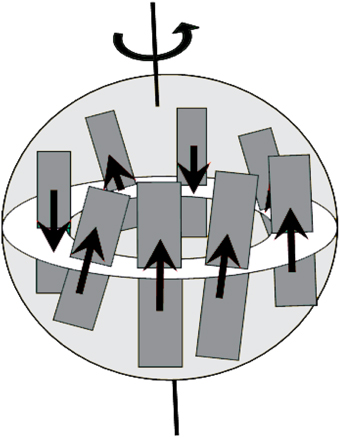
Figure 1. Sketch of the Standard “Domino” model (adapted from Mori et al., 2013).

The potential energy P of the system is composed by two terms: one term models the forcing tendency of each macro-spin to be aligned parallel to the rotational axes; the other term rises from the interaction among macro-spins. We considered two variations of macro-spin interactions: macro-spins interacting pair-wise with their neighbors and macro-spin interacting with all other macro-spins. In the first case the coupling is confined in short distances, hence we have the Short-range Coupling Spins model (SCS), whilst in the second case the coupling is global and the model is known as Long-range Coupled Spins (LCS) model. The potential energy for the SCS model is:

$\begin{array}{cc}P(t)=\gamma {\displaystyle \sum _{i=1}^N{\left(\Omega ·S_i\right)}^2}+\lambda {\displaystyle \sum _{i=1}^N\left(S_i·S_{i+1}\right)}& \left(2\right)\end{array}$

where S_i+1 = S_i when i = N. Here the γ parameter characterizes the tendency of the macro-spins to be aligned with the rotation axis. The squared scalar product in the first summation on R.H.S. of Equation (2) ensures that there is no preferred polarity as it is obvious in the geomagnetic field's case where two stable states of opposite polarity are observed. The λ parameter characterizes the intensity of spin-spin interaction.

The Lagrangian L of the system is:

$\begin{array}{cc}L=\frac{1}{2}{\displaystyle \sum _{i=1}^N{\dot{\theta }}_i}{(t)}^2-\gamma {\displaystyle \sum _{i=1}^N{\left(\Omega ·S_i\right)}^2}-\lambda {\displaystyle \sum _{i=1}^N\left(S_i·S_{i+1}\right)}& \left(3\right)\end{array}$

A Langevin-type equation is set up as follows:

$\begin{array}{cc}\frac{\partial }{\partial t}\left(\frac{\partial L}{\partial {\dot{\theta }}_i}\right)=\frac{\partial L}{\partial {\theta }_i}-\kappa {\dot{\theta }}_i+\frac{\epsilon {\chi }_i}{\sqrt{\tau }}& \left(4\right)\end{array}$

where the term $-\kappa {\dot{\theta }}_i$ describes energy dissipation and the term $\frac{\epsilon {\chi }_i}{\sqrt{\tau }}$ is a random force acting on each spin. The random number χ_i is a Gaussian-distributed random number with zero mean and unit variance which is updated after each correlation time τ. The substitution of Equations (3) into (4) yields the dynamical equations:

$\begin{array}{cc}\begin{array}{l}{\ddot{\theta }}_i-2\gamma \cos {\theta }_i\sin {\theta }_i+\lambda [\cos {\theta }_i(\sin {\theta }_{i-1}+\sin {\theta }_{i+1})\\ -\sin {\theta }_i(\cos {\theta }_{i-1}+\cos {\theta }_{i+1})]+\kappa {\dot{\theta }}_i-\frac{\epsilon {\chi }_i}{\sqrt{\tau }}=0\end{array}& \left(5\right)\end{array}$

where i = 1, 2, …N; θ₀ = θ_N and θ_N+1 = θ₁. (In both models (SCS and LCS), periodic boundary conditions are applied).

The LCS model differs from SCS model in the spin-spin interaction term and all the other terms in Equations (1) and (2) remain identical. The modified potential energy is:

$\begin{array}{cc}P\left(t\right)=\gamma {\displaystyle \sum _{i=1}^N{\left(\Omega ·S_i\right)}^2}+\frac{\lambda }{2N}{\displaystyle \sum _{i=1}^N{\displaystyle \sum _{j>1}\left(S_i·S_j\right)}},& \left(6\right)\end{array}$

and the Langevin equations derived from the modified Lagrangian become:

$\begin{array}{cc}\begin{array}{l}\stackrel{\mathrm{.}}{{\theta }_i}-2\gamma \cos {\theta }_i\sin {\theta }_i+\frac{\lambda }{2N}{\displaystyle \sum _{j\ne i}^N\left(\cos {\theta }_i\sin {\theta }_j-\cos {\theta }_j\sin {\theta }_i\right)}\\ -\kappa \stackrel{.}{{\theta }_i}+\frac{\epsilon {\chi }_i}{\sqrt{\tau }}=0,i=1,\cdots ,N.\end{array}& \left(7\right)\end{array}$

The Equations (5) and (7) are integrated using a 4th-order Runge-Kutta subroutine by applying an internal function of MATLAB (ode45). The initial values of θ_i and time derivatives ${\dot{\theta }}_i$ for the long time series are taken to be uniformly distributed between 0 and 2 π. The values of model parameters: N, γ, λ, κ, ε, and τ are chosen empirically (see Section Some Results and Statistics).

The output of each simulation is the cumulative axial orientation of all macro-spins or axial synchronization, simply named magnetization:

$\begin{array}{cc}M=\frac{1}{N}{\displaystyle \sum _{i=1}^N\left(\Omega ·S_i\right)}=\frac{1}{N}{\displaystyle \sum _{i=1}^{N}cos{\theta }_i}\left(t\right)& \left(8\right)\end{array}$

It corresponds to the normalized axial dipolar moment (ADM) of the geomagnetic field or the first Gauss coefficient $g_1^0$ of the multipolar expansion of the geomagnetic potential.

Inhomogeneous Lebovitz Model

The first example of a rigid rotating system where the dynamo process effect takes place is the homopolar disk dynamo (Moffatt, 1978; Backus et al., 1996). The system is composed of a rigid conductive disk rigidly connected to an axle, which coincides with the disk axis of rotation. A wire in a loop shape is connected mediating two sliding contacts with the disk and the axle (Figure 2A). The system rotates uniformly and the current I flows in the wire and the rigid parts. Depending on the sense of rotation, the initial magnetic field is amplified or decreased monotonically, showing no inversions.

FIGURE 2

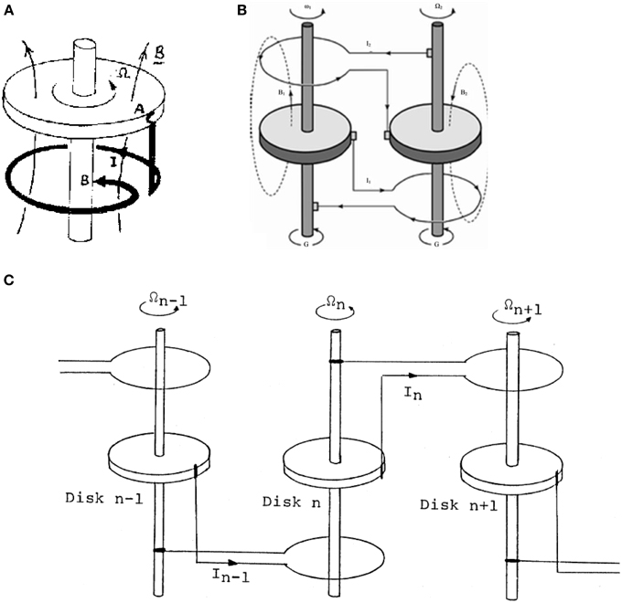
Figure 2. (A) Homopolar disk dynamo (adapted from Leprovost et al., 2005); (B) a sketch of the Rikitake disk dynamo (adapted from Yajima and Nagahama, 2009); (C) a sketch of the IL model consisting of N disks arranged in a circle. The main disk is not shown here (adapted from Shimizu and Honkura, 1985).

Constructing more complicated systems with disk dynamos, one can get interesting results. The first example is the Rikitake two-disk dynamo, widely studied especially from the nonlinear dynamics perspective (Shimizu and Honkura, 1985; Hoshi and Kono, 1988; Hardy and Steeb, 1999; Donato et al., 2009; Danca and Codreanu, 2011). The two disks affect each other through the wires that loop around the respective axes (Figure 2B). The coupling of the disks varies the intensities of the currents that flow in each of them, hence the magnetic field produced by these currents. The corresponding generated time series of magnetic field are chaotic and show magnetic field inversions occasionally. However the spiky oscillations that are observed make the system unrealistic.

Complex magnetic field time series can be obtained by constructing more complex systems with disk dynamos. Shimizu and Honkura (1985) give detailed descriptions for several N-disk systems providing also magnetic field time series generated from numerical simulations. In some of the several N-disk dynamos, the field oscillates chaotically and the spikes are visible. One system in particular produced more realistic magnetic field time series and that is the Inhomogeneous Lebovitz (IL) model. This model, as pointed out by the authors, produces time series that are statistically closer to the paleomagnetic time series. More specifically, they conclude that the statistical distribution of the length of stable polarity periods of the magnetic field time series generated by IL model is very similar to the statistical distribution of stable polarity periods of the Earth's magnetic field.

Basically the IL model is a modification of the Lebovitz model. In this last model, N identical disks are placed on a ring. The disks interact pair-wise only with one of the neighbors in a one-direction interaction. The loop of the i^th disk surrounds the axle of the i^th +1 disk (Figure 2) and the last disk (the N-th disk) interacts with the first disk, i.e., the periodic boundary conditions are assumed. As in the Rikitake two-disks dynamo, the variables of the Lebovitz system are the current intensities I_i and angular velocities Ω_i, where i = 1,…, N. The physical parameters of the system obviously are the electric resistance and inductivity of each loop, mutual inductivity and torques applied on each of the disks. All these physical parameters are the same for all disks. Having homogeneity throughout the system regarding the physical parameters of the disk dynamos, the model is named Homogeneous Lebovitz (HL) model. The non-dimensional dynamical equations of HL model, derived by Cook and Roberts (1970) and Hardy and Steeb (1999), are:

$\begin{array}{ll}\{\begin{array}{l}{\dot{x}}_1+\mu x_1=y_1{x}_N,{\dot{y}}_1=1-x_1{x}_N\\ \dots \dots \dots \dots \dots \dots \dots \dots \dots \dots \\ {\dot{x}}_n+\mu x_n=y_n{x}_{n-1},{\dot{y}}_1=1-x_n{x}_{n-1}\\ \dots \dots \dots \dots \dots \dots \dots \dots \dots \dots \\ {\dot{x}}_N+\mu x_N=y_N{x}_{N-1},{\dot{y}}_N=1-x_N{x}_{N-1}\end{array}& \left(9\right)\end{array}$

where the periodic boundary conditions are applied. In these equations x_i denotes the non-dimensional current intensity of i-th disk dynamo and y_i denotes the non-dimensional angular velocity of the same disk. The only model parameter μ is a non-dimensional quantity that results from the non-dimensioning procedure and characterizes the contribution of the current that flows in the i-th disk in the rate of change of itself. It can be seen that the dynamical equations are mathematically identical to each other that reflects the homogeneity present in the HL system.

If we replace one of the disk dynamos with another one with different physical parameter values, the homogeneity is broken. Let us choose the N-th disk dynamo to be different from the others. Practically the magnetic field generated by the N-th disk is stronger than the field of the other disks and it acts like a dominant magnetic field. The asymmetry or inhomogeneity now present in the system is reflected in the dynamical equations of the IL model (Shimizu and Honkura, 1985):

$\begin{array}{ll}\{\begin{array}{l}{\dot{x}}_1+\mu x_1=m{y}_1{x}_N,{\dot{y}}_1=1-m{x}_1{x}_N\\ \dots \dots \dots \dots \dots \dots \dots \dots \dots \dots \\ {\dot{x}}_n+\mu x_n=y_n{x}_{n-1},{\dot{y}}_1=1-x_n{x}_{n-1}\\ \dots \dots \dots \dots \dots \dots \dots \dots \dots \dots \\ l{\dot{x}}_N+r{x}_N=y_N{x}_{N-1},c{\dot{y}}_N=g-x_N{x}_{N-1}\end{array}& \left(10\right)\end{array}$

Here the parameters m, l, r, c, and g characterize the relative dominance of the main disk compared to the other disk, i.e., parameters give the ratios of the physical parameter values of the main disk to the analogous parameter values of the other minor disks. If all the parameters are equal to unity, we obtain the HL model governing equations. These parameters appear only in the equations of the first and N-th disk because we consider that the dominant disk is in the N-th position and its loop is around the axle of the first disk. The interaction among disks is confined to the interaction with only one the neighbors, hence the IL model is basically a short-range coupling model.

The output of the system is the total magnetisation or the normalized sum of the axial magnetic fields generated by all the disks. The magnetic dipole moment generated by a current I on a loop with surface S, is m = IS. The total magnetisation is proportional to the averaged current intensity because the loops are all with equal surface. The magnetisation M is then:

$\begin{array}{cc}M=\frac{S}{N}{\displaystyle \sum _{i=1}^N{I}_i}& \left(11\right)\end{array}$

where the constant S is the normalizing factor. The magnetisation will take values from -1 to 1 making the results of the IL model comparable with that of SCS/LCS model. A magnetic field reversal occurs when the sign of the averaged current changes from negative to positive (magnetic field flips to normal polarity state) or vice-versa (magnetic field flips to the reversed polarity state).

Some Results and Statistics

Domino Model

The SCS and LCS models have the same six independent parameters. It would be a great challenge to exploit the whole parameter space of the model. Duka et al. (2015) have shown some results of the empirical study of the SCS model dependency on several parameter values taken from defined intervals. Qualitatively similar results are obtained for the LCS model, too. Although we must point out that we have not fully exploited the parameter space for both models.

In order to compare results of the two models, the same set of parameter values are used, precisely: γ = −1, λ = −2, κ = 0.1, ε = 0.4, N = 8, τ = Δt = 0.01 (Duka et al., 2015). The correlation time τ is chosen equal to the time step Δt of equation numerical integration to ensure that the random number χ_i is updated after each time step Δt when the 4th order Runge-Kutta subroutine is called. In order to obtain the long time series of magnetization, we adopted the following initial conditions: random initial θ_i uniformly distributed in the interval (0, 2π) and ${\dot{\theta }}_i=0$.

The full run comprises 30,000,000 time steps and we print the output every 100 time steps, i.e., the full time series has 300,000 time steps. In Figures 3A,B are shown the first 30,000 time steps of two typical series of magnetisation for SCS (a) and LCS (b) model. In order to compare the results of the numerical models with the paleomagnetic data, we have to determine the time scale for each numerical model. In the whole time series generated by SCS model there were observed in average 1339 reversals, while in the LCS time series there were observed in average 660 reversals. The criterion by which the reversals are distinguished is explained in Duka et al. (2015). Dividing the full length of the time series by the number of reversals we obtain the mean time between reversals (mtr). This quantity is simply the statistical mean length of the chrons. The values of mtr for both models are respectively 224 and 454.5 time units. These mean values are derived from the statistical analysis of the reversals. Each of these intervals is considered equivalent to 270,000 years, which is approximately the mtr according to paleomagnetic data (Duka et al., 2015). The typical time series of 300,000 time units long comprises 360 Myr in the case of SCS model and 178 Myr in the case of LCS model. In other words, the time series generated by running the SCS model spans a period of time, in terms of Earth's geological history, nearly twice longer than the time series generated by the LCS model.

FIGURE 3

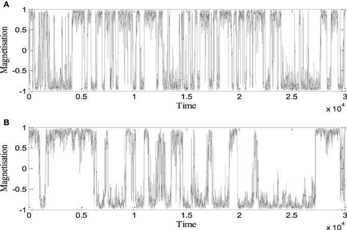
Figure 3. Time series of magnetization generated by (A) SCS model and (B) LCS model. Here are shown values for the first 30,000 time units (adapted from Duka et al., 2015).

The typical feature in both series is the apparently random variance of magnetisation and random change of polarity. It is Power Spectral Density (PSD) of the time series that supplies very valuable information about the statistical behavior of the system in different frequency ranges. The PSDs calculated for long time series (300,000 values) of both SCS and LCS models are shown in Figures 4A,B. One can see that the slopes of power spectra for each series are different for low frequency and high frequency ranges, showing different statistical behavior in low and high frequencies. In the case of the geomagnetic field the difference in statistics between low frequency processes (reversals) and higher frequency processes (in our case SV) would be an argument in favor of the idea that these phenomena are results of different processes in the outer core. This feature of statistic behavior appears not only with SCS/LCS models but with IL model, too.

FIGURE 4

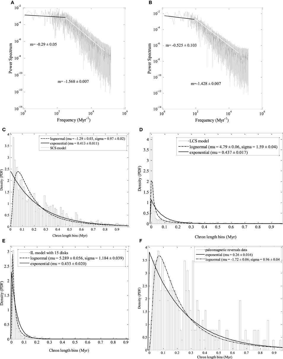
Figure 4. Power spectra density (PSD): of the magnetization series of 300,000 time units generated by (A) SCS model and (B) LCS model with the same values of model parameters; (C) the distribution of chrons length for the SCS model, (D) the distribution of chrons length for the LCS model, (E) the distribution of chrons length of the IL model, (F) the distribution of chrons length of the paleomagnetic time series covering the last 157.53 Myr.

In Figures 4A,B one can see that the statistical behavior of SCS model is qualitatively similar to the behavior of LCS model but quantitatively different. Despite that fact that the time series of the SCS model is twice the length of the time series of the LCS model, the time period they span are of the same order, so they have the same scale.

In order to determine which of the models is statistically closer to the paleomagnetic series of reversals (Cande and Kent, 1995), we have to compare the statistics of reversals of the time series of the models and the paleomagnetic time series which comprises 158 Myr of the past history of the Earth. The power spectra are useless in this case because of the basically different nature between the time series of SCS and LCS models where the magnetisation varies between -1 and 1, and the binary-valued paleomagnetic time series from Cande and Kent record. In Figures 4C–F are shown the distributions of chrons for the time series of the models and Cande and Kent record. We see that both SCS and LCS model have similar reversal statistics being quantitatively different from the statistics of the paleomagnetic time series. So both models are not very accurate in describing the reversal statistics of the geomagnetic field.

Inhomogeneous Lebovitz Model

It can be seen by Equation (10) that the IL model has seven independent parameters, where six of them characterize the physical quantities of the disk dynamos (we use the values μ = 1.0, m = 2.0, l = 2.0, r = 2.0, g = 0.5, c = 1.0; Shimizu and Honkura, 1985), while N is the number of disk dynamos. We used the 4th order Runge-Kutta algorithm to numerically integrate the 2N first order ordinary differential equations of the IL model (Equation 10) with the same ode45 subroutine. A typical time series generated by IL model is given in Figure 5 where N = 15. To generate this long time series we assumed random initial values of non-dimensional current intensities and angular velocities, where the former variables have values one order of magnitude higher than the last variables. When we chose initial values of the same order for all variables, the simulation of the IL model produced time series of monotone magnetisation with no reversals at all. The time series depicted in Figure 5 is 200,000 time units long and it comprises 452 reversals. Then the mean time between reversals for this series is mtr = 442.5 time units, where by considering this mean value equivalent to the geomagnetic field mtr = 270,000 kyr, we deduce that the full run spans nearly 122 Myr.

FIGURE 5

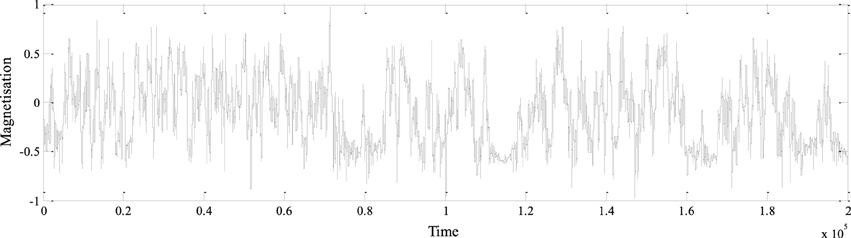
Figure 5. The full run (200,000 time units) generated by the IL model with 15 disk dynamos.

We studied some dependencies of the IL model from the parameter values, but our study does not completely explore all options for the parameter space variations. Especially, we studied the dependency from the number of disks N. When an even number N is used, we noticed that its behavior is very similar to the homogeneous Lebovitz model (see Section Inhomogeneous Lebovitz Model), making the IL model practically identical to the HL model. This result is in accordance with Shimizu and Honkura (1985), who point out the same result, concluding that when there is an even number of disks, the dominance of the main disk vanishes. The main disk effect appears only when we adopt an odd number of disks N. Dropping the N = 1 case, the N = 3 was not appropriate because the magnetisation saturated very early, after the first few thousands of time steps. Then we followed with the next odd natural numbers observing the monotone decrease of mtr with increasing of N. For N = 17, the number of reversals is very high making the model practically non-realistic.

Simulations with different values of the free parameters of the IL model show some interesting results. The increase of μ results in an increase of mtr, i.e., reduced number of reversals. Apparently when the effect of the current intensity on its proper rate of change (see Equation 10) increases, the reversal frequency is diminished. The increase of the values of m, l, c and the decrease of r and g causes an increase of mtr. Higher magnitudes of the first three parameters correspond to enhanced dominance of the main disk while higher magnitudes of the last two parameters correspond to diminished dominance of the same disk. We can conclude that when the dominance of the main disk increases, the system is stabilized and the reversals rate is diminished. On the other hand, when the dominance of the main disk decreases, the system is destabilized and the reversals become more frequent.

The PSDs of all series of magnetisation are qualitatively similar: all of them have a three slope pattern. Quantitatively there are differences especially in the magnitude of the second slope. This part of the power spectra is important because it comprises variations that occur in the time scale from thousands to hundreds of thousands of years, i.e., the time scale of SV. The system with the statistical behavior closest to SHA.DIF.14K model (Pavon-Carasco et al., 2014) is the 15-disk IL model (Figure 6C) and can be seen by comparing the PSDs shown in Figure 6. This implies that the 15-disk IL model should be used to generate the time series to be compared with the SV time series. We also performed simulations with N = 15 disks and different set of parameter values from the initial set. We noticed quantitative changes, because the slopes are different, but with no significant qualitative differences. In Figure 7 is shown the power spectra of one 15-disk IL model. It is evident, after comparing the slope values of this power spectrum with the analogous slope values of the SHA.DIF.14K model (Figure 6A), the time series generated by the IL model with this set of parameter values is statistically very similar to the SV time series making it appropriate to generate long time series of SV.

FIGURE 6

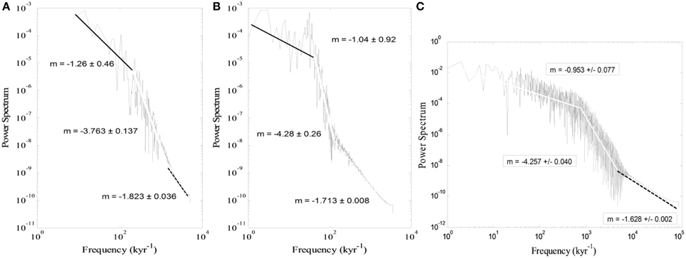
Figure 6. Comparison between the PSD of the time series of: (A) the SHA.DIF.14K model, (B) the LCS model, (C) the IL model with 15 disks.

FIGURE 7

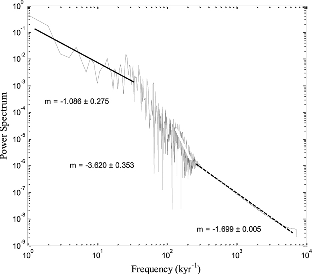
Figure 7. Power spectra (PSD) of the time series generated by the IL model with set of parameter values μ = 0.8, m = 1.8, l = 1.9, r = 2.0, c = 1.0, g = 0.25, N = 15.

The reversal statistics (Figure 4E) shows that the IL model is very close to the SCS and LCS model. The similarity is evident although there are discrepancies when comparing with the reversal statistics of paleomagnetic time series. This result suggests that the IL model is not very accurate in describing the reversal statistics of the geomagnetic field. Actually Shimizu and Honkura (1985) concluded that the IL model, among all the disk dynamo models they studied, is the most appropriate to describe the reversal statistics. However they do not pretend that this model is the best. Our results seem to confirm that this model is not the best for representing the actual reversal statistics.

SV-like Time Series

We generated by the LCS and IL models the time series of magnetisation that are statistically closest to the long time series of SV of the observed Axial Dipolar Moment (ADM) according to paleomagnetic models like as SHA.DIF.14K, at least in the range of parameter values of both models that we have investigated.

In order to compare the results of different models regarding the SV, the time series of axial magnetisation generated by LCS and IL models with proper parameter values and with initial values according to the series of SHA.DIF.14K model that starts at 14,000 BP. The full run comprises 100,000 years, from 14,000 BP to 86,000 terrestrial years in the future (after present, AP). This period of time corresponds to the time-scale of SV. The appropriate parameter values of the LCS model which produce a statistically similar time series with the SHA.DIF.14K time series, found empirically are (Duka et al., 2015): γ = −2.1, λ = −2.0, κ = 0.015, ε = 0.2, τ = 0.01, N = 10. The length of the generated time series which is equivalent to a 100,000-years time series is chosen according to the time scale of LCS model. We considered a set of initial values of angles θ_i, uniformly randomly generated, such that their sum is equal to the initial value of the magnetic dipolar moment (ADM) of the SHA.DIF.14K time series. The initial angular velocities ${\dot{\theta }}_i$, were uniformly randomly generated and filtered until their sum was equal to the initial rate of change of the magnetic dipolar moment. We must emphasize that we do not pretend the set of parameter values we have chosen are unique. From the geodynamo perspective, the magnitudes of the parameters of the “toy” models we study have no relation with the magnitudes of certain quantities which describe the dynamics of the fluid in the outer core. Although these parameters are dimensionless, we do not offer here any theoretical way by which these quantities are connected to other dimensionless quantities, like the fluid dynamics numbers. The same argument is valid for the IL model.

A similar approach is applied for the IL model. The set of parameter values we used is μ = 0.8, m = 1.8, l = 1.9, r = 2.0, c = 1.0, g = 0.25, N = 15. Again this set is found empirically without exploiting large ranges of the whole parameter space. The length of the generated time series spans periods of time as long as 14 millennia (the period of time comprised by the SHA.DIF.14K model), and it is determined considering the time scale of the IL model (see Section Inhomogeneous Lebovitz Model). The initial non-dimensional current intensities and angular velocities of the disks, all uniformly randomly generated, and the magnetisation magnitude Equation (11) is filtered appropriately to fit the initial values of the ADM according to the SV time series.

In both cases we obtained 30 time series respectively. Then we calculated the averaged time series. The SHA.DIF.14K time series and the averaged time series generated by LCS and IL models are all shown in Figure 8.

FIGURE 8

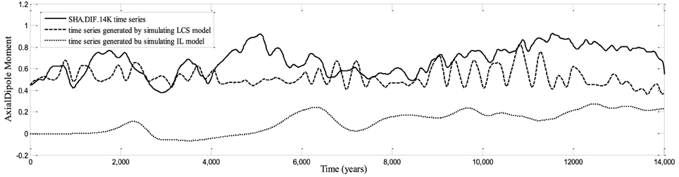
Figure 8. Short time series generated by LCS and IL models compared with the SHA.DIF.14K model time series.

The time series generated by the LCS model approximately reproduces the patterns of SV not only from the statistics point of view, but also by the time dependence of the ADM magnitude. Despite of the quantitative differences, the series have similar statistical behavior (Figures 6A,B). The LCS model seems to nicely describe the SV of the last 14 Myr. The IL model time series on the other hand has the eminent problem that the magnetisation jumps to zero almost immediately from the initial value (this happens in all the time series generated). This discrepancy shows that the IL model is not reliable to reproduce time series of SV that span short geological periods.

The long SV time series is practically a future extension of the actual 14 kyr period initially based on the SHA.DIF.14K model. We performed 30 runs to obtain the averaged long SV time series. The series generated by both models and the respective power spectra are shown in Figures 9A,B, 10A,B. As in Figure 8 it can be seen that the LCS model time series fulfills the non-zero initial conditions, whilst the IL model time series shows the same problem of abruptly jumping to zero ADM soon after the simulation begins. In the IL model time series (Figure 9A), actually occur several reversals that make this series not realistic. In the LCS times series (Figure 10A) a reversal is observed nearly 78,000 years after the hypothetical present, preceded by several millennia of low intensity geomagnetic field. Please note that the exact time of the reversal after the start of the simulation is not the most significant result: because of the high sensitivity of the initial conditions of the system, this could occur at any time. The comparison of power spectra of the SHA.DIF.14K model, LCS and IL models (Figures 6A, 9B, 10B) show that the LCS model (with the chosen parameters) is statistically closer to the paleo-SV series despite the discrepancy in the highest frequencies. What is the most important fact is that several millennia of low intensity geomagnetic dipolar field precede the occurrence of the reversal. This picture supports the idea that reversals might occur during periods of low intensity of the geomagnetic field, as the present feature of the real geomagnetic field. This seems to favor also the view of reversals as outgrowth of SV.

FIGURE 9

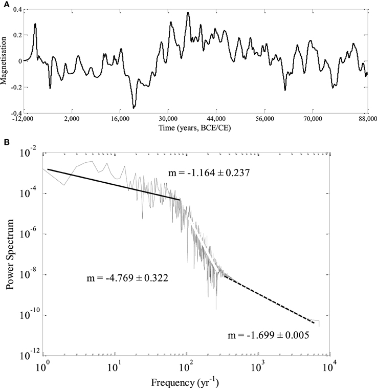
Figure 9. (A) The time series generated by the IL model which comprises 100,000 years, from −12,000 (or BCE) to 88,000 and (B) the Power Spectra of the same time series.

FIGURE 10

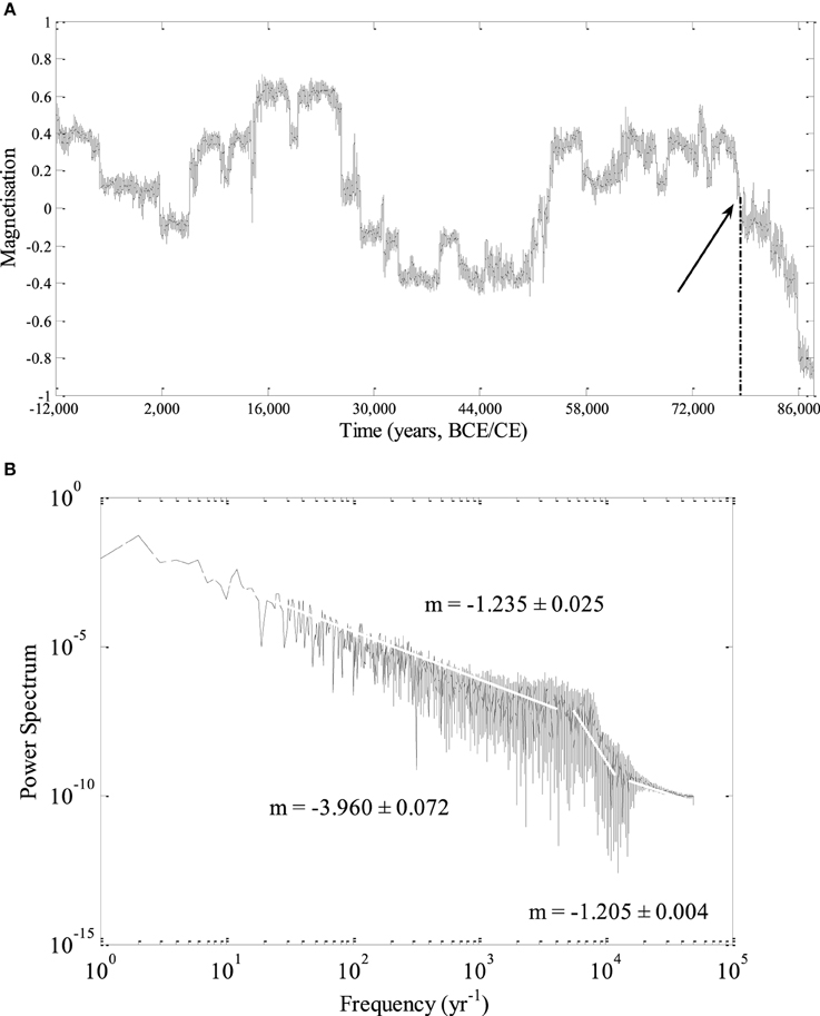
Figure 10. (A) The time series generated by the LCS model which comprises 100,000 years, from −12,000 (or BCE) to 88,000 and (B) the Power Spectra of the same time series.

Discussion and Conclusions

We studied the time series generated by two stochastic models, the LCS model (a version of the “domino” model) and IL model (an extended version of the Rikitake two disk dynamo model). These models consider two distinct ways of dipolar magnetic field generation through collective interaction of dynamo elements: a global interaction of macrospins (LCS model) and a one-sense interaction among neighboring disk dynamos (IL model). In the former case there are implemented secondary interactions like friction and random forces, whilst in the latter case the magnetic field generation is based on interactions among disk dynamos including electric resistance that is analogous to the dissipation in the LCS model. However based on the IL model, more complicated systems including secondary interactions can be explored. The statistical analysis of the magnetisation series generated by both models suggests that the LCS model is more appropriate than IL model to simulate the low frequency processes of the geomagnetic field, i.e., reversals. On the other hand, the power spectra study shows no significant difference between the IL model and LCS model for higher frequency variations. Despite of this, the time series generated by the models showed that the IL model, at least for the considered range of parameters and periods of time of several millenia, is not reliable because of the large discrepancies between the time series of the IL model and paleomagnetic models like SHA.DIF.14K model (Pavon-Carasco et al., 2014). This misfit likely comes from the over simplicity of the IL model. The LCS model on the other hand produces more SV-like time series. We cannot pretend that the time series generated by the LCS and IL models that span more than 86,000 in the Earth's future show what will really occur. However the simulations by both the LCS model and IL model show that the field can be subject to a reversal, when it is preceded by a period of several millennia of low dipole field intensity. Translating these results to the actual geomagnetic field, this conclusion would support the general opinion that reversals occur during geological periods of weak dipolar field, as the present state of the geomagnetic field. The same results also support the view of reversals as outgrowth of SV.

Conflict of Interest Statement

The authors declare that the research was conducted in the absence of any commercial or financial relationships that could be construed as a potential conflict of interest.

Acknowledgments

Some financial support was provided by the Istituto Nazionale di Geofisica e Vulcanologia (INGV) through the funded project LAIC-U.

Supplementary Material

The Supplementary Material for this article can be found online at: https://www.frontiersin.org/article/10.3389/feart.2015.00052

References

Backus, G., Constable, C., and Parker, R. (1996). Foundations of Geomagnetism. New York, NY: Cambridge University Press.

Google Scholar

Barraclough, D., and De Santis, A. (1997). Some possible evidence for a chaotic geomagnetic field from observational data. Phys. Earth. Planet. Inter. 99, 207–220. doi: 10.1016/S0031-9201(96)03215-3

CrossRef Full Text | Google Scholar

Biggin, A. J., van Hinsbergen, D. J. J., Langereis, C. G., Straathof, G. B., and Deenen, M. H. L. (2008). Geomagnetic secular variation in the Cretaceous normal superchron and in the Jurassic. Phys. Earth Planet. Inter. 169, 3–19. doi: 10.1016/j.pepi.2008.07.004

CrossRef Full Text | Google Scholar

Cande, S. C., and Kent, D. V. (1995). A new geomagnetic polarity time scale for the late Cretaceous and Cenozoic. J. Geophys. Res. 97, 13917–13951. doi: 10.1029/92JB01202

CrossRef Full Text | Google Scholar

Christensen, U. R., and Olson, P. (2003). Secular variation in numerical geodynamo models with lateral variations of boundary heat flow. Phys. Earth Planet Inter. 138, 39–54. doi: 10.1016/S0031-9201(03)00064-5

CrossRef Full Text | Google Scholar

Christensen, U. R., and Wicht, J. (2007). “Numerical dynamo simulations,” in Treatise on Geophysics (Core Dynamics), Vol. 8, ed P. Olson (New York, NY: Elsevier), 245–282.

Constable, C. G., and Parker, R. L. (1988). Statistics of the geomagnetic secular variation for the past 5 Ma. J. Geophys. Res. 93, 11569–11582. doi: 10.1029/JB093iB10p11569

CrossRef Full Text | Google Scholar

Cook, A. E., and Roberts, P. H. (1970). The Rikitake two-disk dynamo system. Proc. Cambridge Philoc. Soc. 68, 547–569. doi: 10.1017/S0305004100046338

CrossRef Full Text | Google Scholar

Cox, A. (1969). Geomagnetic reversals. Science 163, 237–245. doi: 10.1126/science.163.3864.237

PubMed Abstract | CrossRef Full Text | Google Scholar

Danca, M. F., and Codreanu, S. (2011). Finding the Rikitake's attractors by parameter switching. arXiv: 1102.2164v1 [nlin.CD].

PubMed Abstract | Google Scholar

Davidson, P. A. (2013). Turbulence in Rotating, Stratified and Electrically Conducting Fluids. New York, NY: Cambridge University Press.

Google Scholar

De Santis, A., and Qamili, E. (2015). Geosystemics: a systemic view of the earth's magnetic field and the possibilities for an imminent geomagnetic transition. Pure Appl. Geophys. 172, 75–89. doi: 10.1007/s00024-014-0912-x

CrossRef Full Text | Google Scholar

De Santis, A., Qamili, E., and Cianchini, G. (2011). Ergodicity of the recent geomagnetic field. Phys. Earth Plan. Inter. 186, 103–110. doi: 10.1016/j.pepi.2011.04.008

CrossRef Full Text | Google Scholar

Donato, S., Meduri, D., and Lepreti, F. (2009). Magnetic field reversals of the earth: a two disk rikitake dynamo model. Inter. J. Modern Phys. B 23, 5492–5503. doi: 10.1142/S0217979209063808

CrossRef Full Text | Google Scholar

Duka, B., De Santis, A., Mandea, A., Isac, A., and Qamili, E. (2012). Geomagnetic jerks characterization via spectral analysis. Solid Earth 3, 131–148. doi: 10.5194/se-3-131-2012

CrossRef Full Text | Google Scholar

Duka, B., Peqini, K., De Santis, A., and Pavon-Carrasco, F. J. (2015). Using “domino” model to study the secular variation of the geomagnetic dipolar moment. Phys. Earth. Planet. Inter. 242, 9–23. doi: 10.1016/j.pepi.2015.03.001

CrossRef Full Text | Google Scholar

Genevey, A., Gallet, Y., Constable, C. G., Korte, M., and Hulot, G. (2008). Archeoint: an upgraded compilation of geomagnetic field intensity data for the past ten millennia and its application to the recovery of the past dipole moment. Geochem. Geophys. Geosyst. 9, Q04038. doi: 10.1029/2007gc001881

CrossRef Full Text | Google Scholar

Glatzmaier, G. A., Coe, R. S., Hongre, L., and Roberts, P. H. (1999). The role of the Earth's mantle in controlling the frequency of geomagnetic reversals. Nature 401, 885–890. doi: 10.1038/44776

CrossRef Full Text | Google Scholar

Glatzmaier, G. A., and Roberts, P. H. (1995). A three-dimensional self-consistent computer simulation of a geomagnetic field reversal. Nature 377, 203–209. doi: 10.1038/377203a0

CrossRef Full Text | Google Scholar

Glatzmaier, G. A., and Roberts, P. H. (1997). Numerical simulations of the geodynamo. Acta Astron. Et Geophys. Uni. Comenianae XIX, 125–143.

PubMed Abstract

Gubbins, D. (1999). The distinction between geomagnetic excursions and reversals. Geophys. J. Int. 137, F1–F3. doi: 10.1046/j.1365-246x.1999.00810.x

CrossRef Full Text | Google Scholar

Guyodo, Y., and Valet, J.-P. (1999). Global changes in intensity of the Earth's magnetic field during the past 800 kyr. Nature 399, 249–252. doi: 10.1038/20420

CrossRef Full Text | Google Scholar

Hardy, Y., and Steeb, W. H. (1999). The rikitake two-disk dynamo system and domains with periodic orbits. Inter. J. Theor. Phys. 38, 2413–2417. doi: 10.1023/A:1026640221874

CrossRef Full Text | Google Scholar

Heimpel, M. H., and Evans, M. E. (2013). Testing the geomagnetic dipole and reversing dynamo models over Earth's cooling history. Phys. Earth Planet. Inter. 224, 124–131. doi: 10.1016/j.pepi.2013.07.007

CrossRef Full Text | Google Scholar

Hoshi, M., and Kono, M. (1988). Rikitake two-disk dynamo system: statistical properties and growth of instability. J. Geophys. Res. 93/B10, 11643–11654. doi: 10.1029/JB093iB10p11643

CrossRef Full Text | Google Scholar

Jacobs, J. A. (1994). Reversals of the Earth's Magnetic Field, 2nd Edn. New York, NY: Cambridge University Press.

Google Scholar

Kageyama, A., and Sato, T. (1997). Velocity and magnetic field structures in a magnetohydrodynamic dynamo. Phys. Plasmas 4, 1569–1575. doi: 10.1063/1.872287

CrossRef Full Text | Google Scholar

Knudsen, M. F., Riisager, P., Donadini, F., Snowball, I., Muscheler, R., Korhonen, K., et al. (2008). Variations in the geomagnetic dipole moment during the Holocene and the past 50 kyr. Earth Plan. Sci. Lett. 272, 319–329. doi: 10.1016/j.epsl.2008.04.048

CrossRef Full Text | Google Scholar

Korte, M., and Constable, C. G. (2005). Continuous geomagnetic field models for the past 7 millennia: 2 CALS7K. Geochem. Geophys. Geosyst. 6, Q02H16. doi: 10.1029/2004gc000801

CrossRef Full Text | Google Scholar

Krijgsman, W., and Kent, D. V. (2004). “Non-uniform occurrence of short-term polarity fluctuations in the geomagnetic field? New results from middle to late miocene sediments of the North Atlantic (DSDP Site 608),” in Timescales of the Paleomagnetic Field, eds J. E. T. Channell, D. V. Kent, W. Lowrie, and J. G. Meert (Washington, DC: American Geophysical Union), 161–174.

Leprovost, N., Dubrulle, B., and Plunia, F. (2005). Instability of the homopolar disk-dynamo in presence of white noise. arXiv:0506050v1 [nlin.CD].

Google Scholar

Lhuillier, F., and Gilder, S. A. (2013). Quantifying paleosecular variation: insights fromnumerical dynamo simulations. Earth Planet. Sci. Lett. 382, 87–97. doi: 10.1016/j.epsl.2013.08.048

CrossRef Full Text | Google Scholar

Merrill, R., and Mcfadden, P. H. (1999). Geomagnetic polarity transitions. Rev. Geophys. 37, 201–226. doi: 10.1029/1998RG900004

PubMed Abstract | CrossRef Full Text | Google Scholar

Merrill, R. T., McElhinny, M. W., and McFadden, P. L. (1996). The Magnetic Field of The Earth: Paleomagnetism, The Core, and The Deep Mantle. San Diego, CA: Academic Press.

Google Scholar

Moffatt, H. K. (1978).Magnetic Field Generation in Electrically Conducting Fluids. London: Cambridge University Press.

Mori, N., Schmitt, D., Wicht, J., Ferriz-Mas, A., Mouri, H., Nakamichi, A., et al. (2013). Domino model for geomagnetic field reversals. Phys. Rev. E 87:012108. doi: 10.1103/physreve.87.012108

PubMed Abstract | CrossRef Full Text | Google Scholar

Naidu, P. (1971). Statistical structure of geomagnetic field reversals. J. Geophys. Res. 76, 2649–2662. doi: 10.1029/JB076i011p02649

CrossRef Full Text | Google Scholar

Nakamichi, A., Mouri, H., Schmitt, D., Ferriz-Mas, A., Wicht, J., and Morikawa, M. (2011). Coupled spin models for magnetic variation of planets and stars. arXiv:1104.5093 [astro-ph.EP].

Google Scholar

Pavon-Carasco, F. J., Osete, M. L., Torta, J. M., and De Santis, A. (2014). A geomagnetic field model of the Holocene based on archaeomagnetic and lava flow data. Earth Planet. Sci. Lett. 388, 98–109. doi: 10.1016/j.epsl.2013.11.046

CrossRef Full Text | Google Scholar

Petrelis, F., Fauve, S., Dormy, E., and Valet, J. P. (2009). A simple mechanism for magnetic field reversals. arXiv: 0806.3756 [physics.geo-ph].

Rüdiger, G., and Hollerbach, R. (2004). The Magnetic Universe: Geophysical and Astrophysical Dynamo Theory. New York, NY: Wiley-VCH.

Google Scholar

Ryan, D. A., and Sarson, G. R. (2007). Are geomagnetic field reversals controlled by turbulence within the Earth's core? Geophys. Res. Lett. 34, L02307. doi: 10.1029/2006GL028291

CrossRef Full Text | Google Scholar

Schmitt, D., Ossendrijver, M. A. J. H., and Hoyng, P. (2001). Magnetic field reversals and secular variation in a bistable geodynamo model. Phys. Earth Planet. Inter. 125, 119–124. doi: 10.1016/S0031-9201(01)00237-0

CrossRef Full Text | Google Scholar

Shimizu, M., and Honkura, Y. (1985). Statistical nature of polarity reversals of the geomagnetic field in coupled-disk dynamo models. J. Geomagn. Geoelectr. 37, 455–497. doi: 10.5636/jgg.37.455

CrossRef Full Text | Google Scholar

Valet, J. P., Plenier, G., and Herrero-Bervera, E. (2008). Geomagnetic excursions reflect an aborted polarity state. Earth Planet. Sci. Lett. 274, 472–478. doi: 10.1016/j.epsl.2008.07.056

CrossRef Full Text | Google Scholar

Yajima, T., and Nagahama, H. (2009). Geometrical unified theory of Rikitake system and KCC-theory. Nonlin. Anal. 71, e203–e210. doi: 10.1016/j.na.2008.10.017

CrossRef Full Text | Google Scholar