When Can a High-Resolution Simulation Over Complex Terrain be Called LES?

The ceaseless rise of computational power leads to a continuous increase of the resolution of the numerical models of the atmosphere. It is found today that operational models are run at horizontal resolutions near 1 km whereas research exercises for flows over complex terrain use resolutions at the hectometer scale. Horizontal resolutions of 100 m or finer have been used to perform Large-Eddy Simulations (LES) for some specific regimes like, e.g., the atmospheric boundary-layer in idealized configurations. However, to use the name “Large-Eddy Simulation” implies to be able to resolve at least the largest turbulent energetic eddies, which is almost impossible to reach with resolutions of the order of 100 m for a real case, where many different processes occur linked to different scales, many of them even smaller than 100 m. Therefore, LES is an inappropriate denomination for these numerical exercises, that may simply be called High-Resolution Mesoscale Simulations.

1. Introduction

Continuous increase of the spatial resolution in mesoscale modeling is allowing currently horizontal resolutions finer than 1 km. This allows modelers to activate the turbulence scheme in three-dimensional (3D) mode and to compute the statistics from the model results. This implies that, sometimes, by an abuse of language, the corresponding simulations are called “Large-Eddy Simulations” (LES), since the traditional tools of the LES community are used. This denomination is seldom found in the written literature [an early example was the one of Chow et al. (2006), that had resolutions of 150 m], probably due to the correcting effect of the review process, but it is often heard in conferences and seminars, followed by unavoidable terminological discussions.

LES have been used by the atmospheric boundary-layer and turbulence scientific community to explore idealized flow configurations at the highest possible resolution. The largest and most energetic eddies must be well resolved, likewise most smaller eddies resulting from non-linear interaction among them, in the so-called energy cascade process that takes place in the Inertial Subrange of the spectrum of motions. The unresolved motions are expected to be homogeneous and isotropic and parameterized accordingly. The simulated regimes are usually run using homogeneous surfaces or simple patterns in the surface heterogeneities, as in Dörnbrack and Schumann (1993) for a wavy surface or Couvreux et al. (2005) and Van Heerwaarden et al. (2014), for terrain discontinuities. A good description of the resolution requirements to perform LES is given in Brasseur and Wei (2010), and a large number of references is listed there referring to other important issues concerning this type of simulations.

The complex-terrain community has made recently a number of LES studies, mainly concerning the Convective Boundary-Layer (CBL) over slopes and in valleys, using resolutions of the order of 50 m and idealized terrain configurations, which fulfill the LES requirements, as in Serafin and Zardi (2010), Schmidli (2013) or Wagner et al. (2014), since the larger and most energetic eddies in this regime have sizes of several hundreds of meters. On the contrary, high-resolution simulations of stably stratified cases over complex terrain, even with resolutions of 100 m like in Vosper et al. (2013) for a valley cold pool, are not called LES, because the largest eddies in that regime are only of the order of some decameters with prescribed realistic surface conditions.

When Chow et al. (2006) called LES a high-resolution simulation case using hectometric resolution, they justified the use of this denomination referring to Wyngaard (2004). In that work Wyngaard suggested that the LES technique could be applied to coarser resolutions that those of LES to address the challenge of the so-called “terra incognita” or “gray zone,” as the horizontal resolutions become finer than 1 km. However, Wyngaard always made a clear distinction between what he labelled high-resolution LES and high-resolution mesoscale modeling, and indicated that the LES technique is another way of parameterizing subgrid motions. The subject of the “gray zone” has been a subject of intense research in the recent years (see Honnert et al., 2011, as an example).

The aim of the paper is clarifying when a complex terrain simulation could be called LES. It will first introduce the concept of the Inertial Subrange of turbulence in Section 2, followed in Section 3 by a discussion about the fact that an LES simulation must have a resolution falling in the Inertial Subrange. Section 4 will explore the scales of some relevant phenomena in complex terrain and see if they are able to be simulated in LES mode with the current numerical capabilities. Finally section 5 will provide the main conclusions of this paper, proposing the more convenient denomination of “High-Resolution Mesoscale Simulations” when using resolutions at the hectometer scale.

2. The Inertial Subrange of Turbulence

The spectrum tensor of turbulence (see Tennekes and Lumley, 1972, for instance) is the Fourier transform of the covariance tensor of the velocity field (R_ij(r, x, t) = $\overline{u_i(\text{x},t)u_j(\text{x}+\text{r},t)}$, the overline corresponding to the Reynolds average),

$\begin{array}{cc}{\psi }_{ij}(k,x,t)={\displaystyle {\int }_{R^3}{R}_{ij}}(r,x,t)e^{-ikr}dr& \left(1\right)\end{array}$

and ψ_ii(k) represents the amount of kinetic energy related to motions of wave number k

$\begin{array}{cc}\frac{1}{2}\overline{u_i^2}=\frac{1}{2}{\displaystyle {\int }_{R^3}{\psi }_{ii}}(k)dk={\displaystyle {\int }_0^{\infty }E}(k)dk& \left(2\right)\end{array}$

where $E(k)=\frac{1}{2}{\int }_{S^2}{\psi }_{ii}(\text{k})dS(\text{k})$ is the scalar energy spectrum, that represents the contribution to the kinetic energy of motions of wave number k, regardless of direction. An evolution equation can be written for this quantity and, assuming that the fluid motion is in statistical equilibrium, a relation can be found for the wave numbers that lie between the scales that bring energy to the flow and those in which this energy is dissipated, but not too close to them, assuming that turbulent motions are isotropic and homogeneous (Kolmogorov, 1941).

$\begin{array}{cc}E(k)\approx {ϵ}^{2/3}{k}^{-5/3};({\Lambda }^{-1}<<k<<{\eta }^{-1})& \left(3\right)\end{array}$

in which Λ is the scale at which energy is supplied to the turbulence, usually scaling well with the dimensions of the largest turbulent eddies, and η is the so-called “Kolmogorov length,” corresponding to the smallest scales in a turbulent flow, where viscosity dominates and turbulent energy is dissipated into heat (Figure 1A). The energy is transferred by non-linear interaction from the large to the small dissipative scales in what is known as “energy cascade.” Introducing Equation (3) in Equation (2) and integrating, we reach the following expression for the dissipation of the turbulent kinetic energy (TKE, $e=\frac{1}{2}\overline{u_i^2}$)

$\begin{array}{cc}ϵ\approx \frac{e^{3/2}}{\Lambda }& \left(4\right)\end{array}$

FIGURE 1

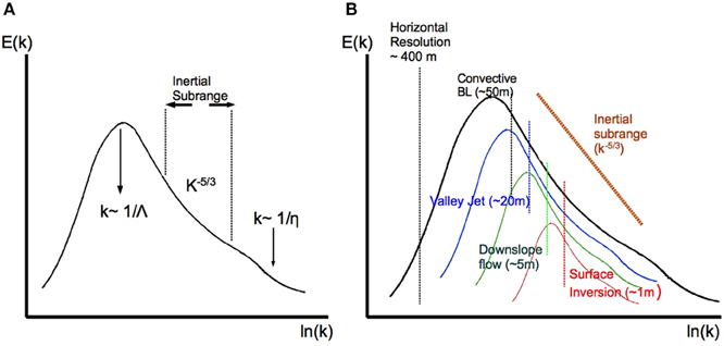
Figure 1. (A) Spectrum for a turbulent flow that has a scale of entrance of energy (Λ), a dissipation scale (η) and a well defined Inertial Subrange. (B) Conceptual representation of the Inertial Subranges corresponding to different structures in a valley flow. The vertical lines indicate the typical scale of the upper size of the Inertial Subrange.

3. LES: Resolution Falling into the Inertial Subrange

A Large-Eddy Simulation (LES) uses a numerical model of a turbulent flow, with the aim of explicitly representing the largest and most energetic scales of turbulence. This way the upper part of the Inertial Subrange is captured and, if the later is well defined until the dissipation scales, the Kolmogorov theory is of application. The Smagorinsky-Lilly closure can be applied in first order models (see in Wyngaard, 2004) and the dissipation formula (4) can be used in models using a TKE-equation (1.5 order models, as in Cuxart et al., 2000), since in both cases it is implicitly assumed that resolved energy production and parameterized dissipation are in equilibrium.

It is therefore clear that an LES must be capturing explicitly at least the largest turbulent eddies of the Inertial Subrange. This is extremely difficult even for the simplest configurations. Let us illustrate the problem taking a simple atmospheric CBL for discussion. Assuming that the surface heating is able to generate a CBL of a height approximately of 1000 m, the well-developed thermals may have vertical dimensions of several hundreds of meters. The non-linear interaction between convective eddies will generate smaller eddies due to the energy cascade described above. This process can be successfully simulated using resolutions of tens of meters in which the smallest resolved eddies will have scales of at most 100 m, eddies that probably will already be homogeneous and isotropic, allowing the full application of the Kolmogorov theory.

However, even in this simple case there are two layers where the resolution is usually not able to capture the largest turbulent eddies in them: the surface layer near the ground and the entrainment zone at the top of the CBL. In the first case the eddies are smaller as they are closer to the surface and are not captured by the aforementioned resolution of some tens of meters (see a detailed discussion in Brasseur and Wei, 2010). The classical solution in this case is to impose the phenomenological knowledge that the similarity theory provides to overcome this limitation or to use hybrid approaches (Bechmann and Sorensen, 2010). In the case of the entrainment zone, stable stratification limits the vertical size of the eddies and introduces anisotropy in the turbulence. The solutions would be either to increase the resolution—and, as long as the latter is too low, the numerical results may not match well with the available observations (Sullivan et al., 1998)—or to introduce a parameterization for this effect in the layer.

In a general case, as the size of the most energetic eddies of a regime becomes smaller, the finer must be the resolution of the LES. For instance a weakly stably stratified nocturnal boundary layer has the more energetic eddies that have typical sizes below 100 m, slightly anisotropic, and that need resolutions of the order of 5 to 10 m to be well resolved, still having the problem of the surface layer (Beare et al., 2006). For a more stable nocturnal boundary layer, eddies are typically of few meters, even for slope flows, and the requested resolutions for a LES must be clearly finer than 5 m (Jimenez and Cuxart, 2005).

When a simulation is using a resolution that is not capturing the most energetic turbulent eddies of all the different configurations that it contains, then there is a range of energetic motions that cannot be parameterized using the Kolmogorov theory. We would say that in this case the resolution falls to the left of the beginning of the Inertial Subrange (see Figure 1). If this limitation happens extensively for a simulation, then it cannot be called LES anymore, and the 3D subgrid turbulence scheme is just a parameterization of the unresolved motions not sustained on the Kolmogorov theory and therefore, conceptually similar to a pure one-dimensional approach.

There is also the issue of the anisotropy of the grid mesh. LES must have a grid that captures energetic eddies and those not resolved are supposed to be isotropic and homogeneous. A largely anisotropic grid would allow anisotropic eddies to be unresolved and it is advisable to refrain using grids that depart too much from isotropy [customarily never more than a 1 to 4 ratio between vertical and horizontal resolution, Baggett et al. (1997)]. This requirement is sometimes relaxed near the surface, where similarity theory is used.

In the next section we will discuss about how a real case simulation for complex terrain is very often not fulfilling the LES requirements, and why, in consequence, they cannot be called LES.

4. Characteristic Scales of the Regimes Over Complex Terrain

The examples cited in the previous section were mostly for flat terrain Boundary-Layer regimes and the LES resolution requirements became evident, especially near the surface and in stably stratified conditions.

Figure 2 is a vertical cross section from a simulation for La Cerdanya Valley in the Pyrenees (Martinez-Villagrasa et al., 2015), using a horizontal resolution of 400 m and a vertical resolution of 5 m, with a 1.5 order one-dimensional turbulence scheme activated, a setup identical to the one described in Jimenez and Cuxart (2014) for a narrow valley in the Northern Pyrenees. We call this a high-resolution mesoscale simulation, as it is capturing phenomena with scales between one and 40 km (mesogamma and mesobeta structures). This approach, with very anisotropic grid elements, cannot be called LES by definition, since the grid structure should not depart too much from isotropy, and because many relevant eddies have scales well below 400 m and could never be captured by this discretization setup. However, the dynamic equations and the one-dimension turbulence scheme are able to provide a description of the flows that is very close to reality.

FIGURE 2

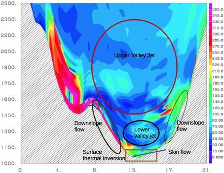
Figure 2. Vertical cross-section of the wind direction for a simulation of La Cerdanya valley in the Pyrenees, for a cross valley direction at night. Some main structures are indicated. The vertical scale is in meters and the horizontal scale in kilometers.

Some of the main structures taking place in a wide mountainous valley at night can be seen in Figure 2, where the wind direction is shown. The valley bottom has near 5 km width and 25 km length, whereas the distance between the tops of the surrounding mountain ranges is close to 20 km and the vertical distance from peaks to valley is 1500 m. Five main structures have been signaled in the Figure and some relevant scales are listed in Table 1. A conceptual graph indicating a typical start of the Inertial subrange for each structure is given in Figure 1B. For a real flow containing all these structures the spectrum may be a superposition of the above-mentioned spectra and, consequently, it may not show an inertial subrange.

TABLE 1

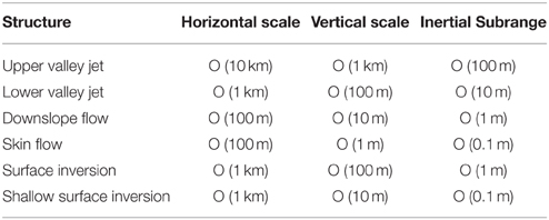
Table 1. Valley flow structures: order of magnitude of sizes and of related inertial subrange.

The upper valley jet is a mesobeta structure, covering usually the whole length of the valley and many times connected to adjacent valley structures, that can exist at day and at night. Its depth is of several hundred meters and a simulation with a resolution near 100 m could resolve well the largest eddies and perform a LES of this structure. The lower valley jet results from the accumulation of cold air at night flowing downvalley, many times above a shallow thermal inversion, with some intermittent mixing events between the two structures during the night. Typically they have a depth of 50–100 m and a LES of them could be made with resolutions of the order of 10–20 m.

All the other important structures signaled in Figure 2 have much smaller scales and it is currently not possible to be able to capture the most energetic eddies related to them with the setups that we are discussing here. All of them are shallow and in contact with the surface, therefore they adapt to the topographical characteristics of the terrain. These are usually broken structures, anisotropic (shallow and elongated) with energetic eddies that have a short size in the vertical. To make an LES of them, resolutions of the order of 5–10 m would be a minimum requirement. Furthermore, no generally accepted similarity expressions exist, due to the high influence of the local effects, although work is in progress for some simple configurations, such as in Grisogono et al. (2007), but these approaches seem still not to be well adjusted to general observations (Nadeau et al., 2013).

Specifically, for downslope flows and deep surface inversions, any LES study of them would require vertical resolutions of the order of at least 5 m, keeping in mind that grid meshes must not be too anisotropic. When addressing skin flows or shallow inversions, which are cases of strongly stably stratified regimes, the resolution should be of the order of 1 m or finer.

5. The Current State: High-resolution Mesoscale Simulations

Arguments have been given above about why activating a 3D turbulence scheme does not directly imply that the simulation becomes an LES. The latter should capture the most energetic eddies of all the structures present in the simulated field. If it is a real case, it will include daytime, nighttime and the morning and evening transitions, with a large variety of structures of different scales, many of them with sizes of only a few meters. Besides, to perform an LES implies using a quasi-isotropic grid mesh, since it is necessary that the resolved eddies belong to the upper part of the Inertial Subrange. The only usual exception is to impose the phenomenological knowledge close to the surface by use of the similarity theory, not well established yet over complex terrain for strongly stratified conditions.

To use resolutions of some hundreds of meters has been a hot research topic in the last decade, since it is still unclear when it is more convenient to use a parameterized 1D turbulence scheme or to activate a 3D turbulence scheme that may resolve part of the most energetic eddies, in what is called the “gray zone” area. With these resolutions, for turbulence eddies of scales of 100 m or smaller, a 3D scheme will not add much to the performance of a 1D scheme, because the horizontal gradients will already be taken into account by the advection scheme of the model. On the other hand, energetic eddies of several hundreds of meters will be resolved by the model and highly parameterized 1D turbulence schemes may also account for their effects, leading to what is known as the “double-counting” problem (Honnert et al., 2011).

A good practice is to inspect very carefully the characteristics of the regime that is the subject of study before fixing the key options in the simulation setup. In complex terrain daytime real flows, eddies will be of relatively large dimension and the choice of a 3D turbulence scheme may be advisable, even if the resolution is as low as some hundreds of meters. In this case we would be in the frame of what is called “Very-Large Eddy simulation” (VLES, Smolarkiewicz and Prusa, 2002), for which the resolution falls outside but near the Inertial subrange and the 3D scheme is still just a parameterization.

For the morning and evening transitions, as well as for the nighttime, most eddies are of scales of some decameters. This resolution is currently not affordable for the vast majority of numerical studies over real complex terrain. Furthermore, many of these eddies are strongly anisotropic, having a horizontal dimension much larger than the vertical one. Therefore, many of the horizontal characteristics will be approximately well captured by the dynamical equations. Instead, the turbulence exchanges will be of small dimension, sometimes generated by vertical gradients and many times in an intermittent manner. Therefore, here it is perhaps more advisable to choose a 1D-turbulence scheme to save computational resources, although a 3D scheme with a highly parameterized mixing length will probably be acting equivalently, due to the very small values of the horizontal gradients. In this case we would be talking about a high-resolution mesoscale simulation, since the horizontal resolution is clearly coarser than the scales of the larger eddies at the beginning of the Inertial Subrange.

Summarizing, for simulations of real flows over complex terrain:

• A simulation over complex terrain with horizontal resolution of some hectometers with a 3D turbulence scheme is not an LES, since the resolved motions do not belong to the Inertial Subrange of the flow.

• In the daytime, with prevailing convective motions, simulations with resolutions of the order of 50 m or finer can be considered LES, whereas coarser resolutions of a few hectometers correspond to Very-Large Eddy Simulations (VLES), as the smaller resolved motions are into the Inertial Subrange.

• For other regimes, especially at night, simulations at the hectometer resolution have resolved eddies that are far from the Inertial Subrange. The turbulence is highly parameterized, either with a 1D scheme or with a 3D scheme. Even finer resolutions fail to capture the inertial subrange of shallow structures near the surface. In this case an LES is usually not possible with the computational capabilities at hand of most research teams. These numerical exercises should be called more properly “High-Resolution Mesoscale Simulations.”

Funding

This article has received financial support of the Spanish Government, supplement with European FEDER funds, through Grant CGL2012-37416-C04-01.

Conflict of Interest Statement

The author declares that the research was conducted in the absence of any commercial or financial relationships that could be construed as a potential conflict of interest.

Acknowledgments

Maria Antonia Jiménez is acknowledged for providing the vertical cross-section used to build Figure 2.

References

Baggett, J. S., Jimenez, J., and Kravchenko, A. G. (1997). Resolution Requirements in Large-eddy Simulations of Shear Flows. Stanford: Turbulence Research Center.

Google Scholar

Beare, R. J., Macvean, M. K., Holtslag, A. A., Cuxart, J., Esau, I., Golaz, J. C., et al. (2006). An intercomparison of large-eddy simulations of the stable boundary layer. Boundary Layer Meteorol. 118, 247–272. doi: 10.1007/s10546-004-2820-6

CrossRef Full Text | Google Scholar

Bechmann, A., and Sorensen, N. N. (2010). Hybrid RANS/LES method for wind flow over complex terrain. Wind Energy 13, 36–50. doi: 10.1002/we.346

CrossRef Full Text | Google Scholar

Brasseur, J. G., and Wei, T. (2010). Designing large-eddy simulation of the turbulent boundary layer to capture law-of-the-wall scaling. Phys. Fluids 22, 021303. doi: 10.1063/1.3319073

CrossRef Full Text | Google Scholar

Chow, F. K., Weigel, A. P., Street, R. L., Rotach, M. W., and Xue, M. (2006). High-resolution large-eddy simulations of flow in a steep Alpine valley. Part I: methodology, verification, and sensitivity experiments. J. Appl. Meteorol. Climatol. 45, 63–86. doi: 10.1175/JAM2322.1

CrossRef Full Text | Google Scholar

Couvreux, F., Guichard, F., Redelsperger, J. L., Kiemle, C., Masson, V., Lafore, J. P., et al. (2005). Water-vapour variability within a convective boundary-layer assessed by large-eddy simulations and IHOP 2002 observations. Q. J. R. Meteorol. Soc. 131, 2665–2693. doi: 10.1256/qj.04.167

CrossRef Full Text | Google Scholar

Cuxart, J., Bougeault, P., and Redelsperger, J. L. (2000). A turbulence scheme allowing for mesoscale and large-eddy simulations. Q. J. R. Meteorol. Soc. 126, 1–30. doi: 10.1002/qj.49712656202

CrossRef Full Text | Google Scholar

Dörnbrack, A., and Schumann, U. (1993). Numerical simulation of turbulent convective flow over wavy terrain. Boundary Layer Meteorol. 65, 323–355.

Google Scholar

Grisogono, B., Kraljevic, L., and Jericevic, A. (2007). Notes and correspondencethe low-level katabatic jet height versus MoninObukhov height. Q. J. R. Meteorol. Soc. 133, 2133–2136. doi: 10.1002/qj.190

CrossRef Full Text | Google Scholar

Honnert, R., Masson, V., and Couvreux, F. (2011). A diagnostic for evaluating the representation of turbulence in atmospheric models at the kilometric scale. J. Atmos. Sci. 68, 3112–3131. doi: 10.1175/JAS-D-11-061.1

CrossRef Full Text | Google Scholar

Jimenez, M. A., and Cuxart, J. (2005). Large-eddy simulations of the stable boundary layer using the standard Kolmogorov theory: range of applicability. Boundary Layer Meteorol. 115, 241–261. doi: 10.1007/s10546-004-3470-4

CrossRef Full Text | Google Scholar

Jimenez, M. A., and Cuxart, J. (2014). A study of the nocturnal flows generated in the north side of the Pyrenees. Atmos. Res. 145, 244–254. doi: 10.1016/j.atmosres.2014.04.010

CrossRef Full Text | Google Scholar

Kolmogorov, A. N. (1941). “Dissipation of energy in locally isotropic turbulence,” in Doklady Akademii Nauk SSSR, Vol. 32 (Moscow), 16–18.

Martinez-Villagrasa, D., Conangla, L., Tabarelli, D., Jimenez, M. A., Miro, J. R., Zardi, D., et al. (2015). “Slope and valley flows at the Cerdanya valley in the Pyrenees,” in 33rd International Conference on Alpine Meteorology (Innsbruck).

Nadeau, D. F., Pardyjak, E. R., Higgins, C. W., and Parlange, M. B. (2013). Similarity scaling over a steep alpine slope. Boundary Layer Meteorol. 147, 401–419. doi: 10.1007/s10546-012-9787-5

CrossRef Full Text | Google Scholar

Schmidli, J. (2013). Daytime heat transfer processes over mountainous terrain. J. Atmos. Sci. 70, 4041–4066. doi: 10.1175/JAS-D-13-083.1

CrossRef Full Text | Google Scholar

Serafin, S., and Zardi, D. (2010). Daytime heat transfer processes related to slope flows and turbulent convection in an idealized mountain valley. J. Atmos. Sci. 67, 3739–3756. doi: 10.1175/2010JAS3428.1

CrossRef Full Text | Google Scholar

Smolarkiewicz, P. K., and Prusa, J. M. (2002). VLES modelling of geophysical fluids with nonoscillatory forward-in-time schemes. Int. J. Numer. Methods Fluids 39, 799–819. doi: 10.1002/fld.330

CrossRef Full Text | Google Scholar

Sullivan, P. P., Moeng, C. H., Stevens, B., Lenschow, D. H., and Mayor, S. D. (1998). Structure of the entrainment zone capping the convective atmospheric boundary layer. J. Atmos. Sci. 55, 3042–3064. doi: 10.1175/1520-0469(1998)055<3042:SOTEZC>2.0.CO;2

CrossRef Full Text | Google Scholar

Tennekes, H., and Lumley, J. L. (1972). A First Course in Turbulence. Cambridge, MA: MIT press.

Google Scholar

Van Heerwaarden, C. C., Mellado, J. P., and De Lozar, A. (2014). Scaling laws for the heterogeneously heated free convective boundary layer. J. Atmos. Sci. 71, 3975–4000. doi: 10.1175/JAS-D-13-0383.1

CrossRef Full Text | Google Scholar

Vosper, S., Carter, E., Lean, H., Lock, A., Clark, P., and Webster, S. (2013). High resolution modelling of valley cold pools. Atmos. Sci. Lett. 14, 193–199. doi: 10.1002/asl2.439

CrossRef Full Text | Google Scholar

Wagner, J. S., Gohm, A., and Rotach, M. W. (2014). The impact of horizontal model grid resolution on the boundary layer structure over an idealized valley. Mon. Weather Rev. 142, 3446–3465. doi: 10.1175/MWR-D-14-00002.1

CrossRef Full Text | Google Scholar

Wyngaard, J. C. (2004). Toward numerical modeling in the Terra Incognita. J. Atmos. Sci. 61, 1816–1826. doi: 10.1175/1520-0469(2004)061<1816:TNMITT>2.0.CO;2

CrossRef Full Text | Google Scholar