Non-linear Topographic Effects in Two-Layer Flows

Introduction

Some phenomena in the lower atmosphere may be approximately described by motion of a dense lower layer surmounted by a deep upper layer of approximately uniform density. The processes that occur in such flows can be described by the analysis of flows consisting of two layers of uniform density and velocity with a rigid upper surface. This constitutes the simplest form of density-stratified flow, and contains a number of phenomena that are prominent in more complex flows, such as hydraulic jumps. Here we report results of a study of two-layer stratified flow over isolated topography that incorporate some recent results on hydraulic jumps, namely improved (and justifiably correct) models of such jumps, for all density ratios. The Boussinesq approximation (namely, that the fluid density is assumed uniform except where multiplied by g) is not made here. This enables a better appreciation of the effects of density variation, particularly in hydraulic jumps. The presence of the upper boundary provides some simplifications, and while not being particularly relevant to the atmosphere, can be removed to an arbitrarily high level.

A general description of two-layer flows over topography is given in Chapter 3 (specifically, Section 3.6 of Baines, 1995, 1998), using models of hydraulic jumps that were prevalent at that time. The cases considered were those of two-layer flow with uniform velocity that commenced from a state of rest over an isolated, long obstacle, and concentrated on the “Boussinesq limit” where the density difference is very small. The resulting flows were described in terms of the parameters r, F₀, and H_m, where (generalizing to all densities)

$\begin{array}{ll}r=\frac{d_{10}}{D},H_m=\frac{h_m}{d_{10}},F_0=\frac{U}{c_0},c_0^2=\frac{\Delta \rho g}{\frac{{\rho }_1}{d_{10}}+\frac{{\rho }_2}{d_{20}}},& \left(1.1\right)\hfill \end{array}$

where ρ₁ and ρ₂ denote the lower and upper layer densities respectively, Δρ = ρ₁ − ρ₂, U is the initial fluid velocity in the frame of the obstacle, D the total depth, g gravity, d₁₀ and d₂₀ = D − d₁₀ the initial undisturbed lower and upper layer thicknesses, and h_m is the height of the highest point of the obstacle. c₀ denotes the speed of long waves in two-layer fluid at rest. A definition sketch with velocities given in the frame of the topography is given in Figure 1. If the lower layer is thinner than the upper layer, the sudden onset of flow generates an hydraulic jump upstream, and the appropriate solutions for the flow depend on the dynamical properties of such jumps.

FIGURE 1

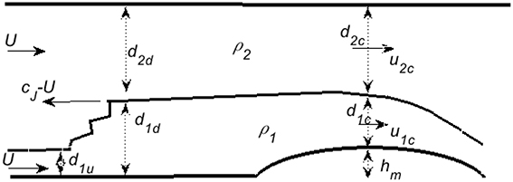
Figure 1. A representative diagram showing the nature of the flows considered in this analysis. These are hydrostatic two-layer flows with a rigid lid, forced by flow over a long obstacle. See text for notation.

Section Hydraulic Jumps in Two-layer Flows gives a summary of the properties of such jumps based on recent analysis by Borden and Meiburg (2013) for Boussinesq flows, which have been generalized to all densities by the first author of this paper in Baines (2015). A study of jumps in continuously stratified fluids in the Boussinesq limit has been described by White and Helfrich (2014) using the Dubreil-Jacotin-Long equations, which provides an interesting contrast to the two-layer model employed here.

The basic equations for time-dependent non-linear two-layer flow are presented in Section Equations for Time-Dependent Non-linear Two-Layer Flow, and using the new model of hydraulic jumps, the methodology for computing the properties of flow over a single obstacle is presented in Section Two-Layer Flow over a Single Obstacle. The results are given in terms of F₀ − H_m diagrams in Section Results, and the conclusions are summarized in Section Conclusions.

Flows close to the Boussinesq limit are more relevant to applications to the atmosphere and ocean, where (potential) densities do not vary greatly, and these have been more closely studied in the past, but non-Boussinesq flows show some interesting differences. Flows where the lower layer is thinner than the upper are perhaps the most relevant to atmospheric and oceanic situations, and these are found to be the more complex in the non-Boussinesq case. The new hydraulic jump model may be extended to include mixing within (or downstream of) the jump, and hence also applied to flow over topography, but this has not been done here.

Hydraulic Jumps in Two-layer Flows

This section summarizes the results given in Baines (2015). An hydraulic jump in two-layer fluids is here defined to be a flow structure that represents a transition between two steady uniform two-layer flow states (this may be extended to include an undular bore that leaves a downstream wavetrain, in which case the downstream flow state is taken to be the average layer thickness and velocities). A definition sketch for jumps is shown in Figure 2, which shows variables and velocities in the frame of the jump: subscripts 1 and 2 denote the lower and upper layers, subscripts “u” and “d” denote upstream and downstream, and u and d with subscripts denote layer velocities and thicknesses (see Figure 1). p_su and p_sd denote the pressure at the upper surface upstream and downstream respectively. Our objective is to obtain the flow properties downstream of the jump in terms of its amplitude, where the latter is measured by the increment in lower-layer thickness. We make the following assumptions: (1) the jump is steady in a reference frame moving with it; (2) the top and bottom surfaces are horizontal through the jump, with no surface stress, and (3) the layers maintain their identity through the jump, with negligible exchange of fluid between them. With these assumptions we have

$\begin{array}{ll}{d}_{1u}+d_{2u}=D=d_{1d}+d_{2d},d_{id}{u}_{id}=d_{iu}{u}_{iu},i=1,2.& \left(2.1\right)\hfill \end{array}$

and from assumption (2) we have that the momentum flux S must be uniform (see Baines, 1995, 1998), so that

$\begin{array}{l}S={\displaystyle {\int }_0^D}(p+\rho u^2)\text{d}z=\text{constant}\\ =p_{su}D+\frac{1}{2}\Delta \rho g{d}_{1u}^2+{\rho }_1{u}_{1u}^2{d}_{1u}+{\rho }_2{u}_{2u}^2{d}_{2u}+\frac{1}{2}{\rho }_{2}g{D}^2,& \left(2.2\right)\hfill \end{array}$

which is equal to the same expression on the downstream side. This equation introduces an additional variable, p_su − p_sd, which needs to be determined by other considerations:

$\begin{array}{l}{p}_{su}-p_{sd}=\frac{\Delta \rho g}{2D}\left(d_{1d}^2-d_{1u}^2\right)+{\rho }_1\left(u_{1d}^2{d}_{1d}-u_{1u}^2{d}_{1u}\right)∕D\\ +{\rho }_2\left(u_{2d}^2{d}_{2d}-u_{12}^2{d}_{2u}\right)∕D.& \left(2.3\right)\hfill \end{array}$

FIGURE 2

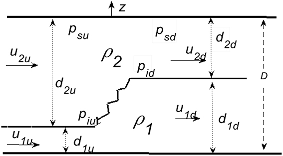
Figure 2. Notation sketch for hydraulic jumps, with velocities relative to a frame of reference moving with the jump. For the subscripts, layer 1 is the lower, layer 2 the upper, “u” denotes upstream, “d” downstream, and for the pressure, “s” denotes surface, and “i” the interface.

There have been essentially three previous attempts which have involved assumptions about the dynamics to give expressions for p_su–p_sd. The first was by Yih and Guha (1955) (the problem is 60 years old!), who assumed that the flow within the jump was hydrostatic, and that p_s varies linearly with d₂; the second was by Chu and Baddour (1977) and Wood and Simpson (1984), who assumed that all the energy dissipation in the jump was contained within the expanding (lower) layer, and the third was by Klemp et al. (1997), who assumed that all the energy dissipation was contained in the contracting (upper) layer. These assumptions gave different results, and with hindsight, none of them is correct, though as it turns out, the model of Klemp et al. is a good approximation in the Boussinesq limit. See Baines (2015) for details.

The novel approach from Borden and Meiburg (2013) was to consider a vorticity budget of the jump, and show, for the Boussinesq case, that the vorticity generation is independent of the pressure difference across the jump, and Equation (2.3) is not needed. In the non-Boussinesq case (Baines, 2015), the vorticity generated is determined by this pressure difference, and provides an expression for it. Specifically, if the vorticity equation (without friction) is written in the form

$\begin{array}{ll}\mathbf{u}.\nabla \omega =-\nabla x\left(\frac{1}{\rho }\nabla p\right),& \left(2.4\right)\hfill \end{array}$

and integrated over the area A of the jump, using the Gauss and Stokes theorems it reduces to

$\begin{array}{ll}\int \omega {\mathbf{u}}_{\bullet }d\mathbf{S}=-\int \frac{1}{\rho }\nabla p.d\mathbf{l},& \left(2.5\right)\hfill \end{array}$

where S denotes the normal vector to the boundary of A, and l denotes the vector along it, in the anti-clockwise sense. Since the density is uniform in each layer, and if u_1u = u_2u, this equation reduces to

$\begin{array}{l}\frac{1}{2}\left(u_{2d}^2-u_{1d}^2\right)=\left[\frac{1}{{\rho }_2}-\frac{1}{{\rho }_1}\right]\left(p_{iu}-p_{id}\right)\\ =\frac{\Delta \rho }{{\rho }_1}\frac{p_{su}-p_{sd}}{{\rho }_2}+\frac{\Delta \rho g}{{\rho }_1}\left(d_{1d}-d_{1u}\right),& \left(2.6\right)\hfill \end{array}$

where p_id and p_iu denote the pressures at the downsteam and upstream interfaces respectively, which may be related hydrostatically to the surface pressures. This analysis obviates the necessity for the various different assumptions made or proposed by Yih and Guha (1955), Wood and Simpson (1984), Klemp et al. (1997) and Li and Cummins (1998).

From Equations (2.3) and (2.6) we may eliminate p_su − p_sd, and obtain the expression for the speed c_J of an hydraulic jump (see Figure 1) moving into fluid at rest:

$\begin{array}{ll}{\left(\frac{c_J}{c_0}\right)}^2=\frac{r_d^2{\left(1-r_d\right)}^2\left[1-r_u\left(1-\frac{{\rho }_2}{{\rho }_1}\right)\right]\left[1+\left(\frac{{\rho }_1}{{\rho }_2}-1\right)\frac{\left(r_u+r_d\right)}{2}\right]}{r_u\left(1-r_u\right)\left[\frac{\left(r_u+r_d\right)}{2}-r_u{r}_d+\left(\frac{{\rho }_1}{{\rho }_2}-1\right)r_u{r}_d{\left(1-r_d\right)}^2-\left(1-\frac{{\rho }_2}{{\rho }_1}\right)r_d^2\left(1-r_u\right)\left(1-r_d\right)\right]},& \left(2.7\right)\hfill \end{array}$

where c₀ is the linear wavespeed as in Equation (1.1) and r_u = d_1u∕D, r_d = d_1d∕D. Borden and Meiburg (2013) termed their Boussinesq model for the jump speed the VS, or “Vortex Sheet” model, so that it is appropriate to term this model the FVS, or “Full Vortex Sheet” model.

Some representative plots for c_J∕c₀ are shown in Figure 3, as a function of r_d, for a range of density ratios. Note that all of these curves attain a maximum speed, but exist at larger amplitude, up to a maximum amplitude where the energy loss in each layer vanishes. For each curve, the maximum energy loss in each layer within the jump coincides with the point of maximum speed. Further, relative to the reference frame of the jump, the flow immediately downstream is subcritical for jump amplitudes r_d less than that of maximum speed (denoted r_dms), but is supercritical for jumps with amplitudes greater than or equal to that maximum speed (r_d ≥ r_dms). This means that, on the dashed part of the curves, disturbances from downstream cannot propagate up to these jumps and affect them. Such jumps, if they did exist, would also be expected to be unstable, and degenerate to a jump of maximum speed. For these reasons, the jumps with r_d ≥ r_dmsare shown dashed in Figure 3, and are not significant in the following analysis. More details are given in Baines (2015).

FIGURE 3

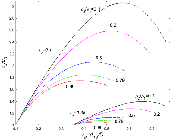
Figure 3. Some representative jump speeds as a function of jump amplitude, moving into fluid at rest, for a range of density ratios (ρ₂∕ρ₁ = 0.1, 0.2, 0.5, 0.79, 0.99). The upstream lower layer thicknesses are given by r_u = d_1u/D = 0.1 and 0.35. The dashed portions of the curves denote the regions where jump speed decreases with increasing amplitude. This makes them potentially unstable. Further, for these dashed curves, the flow is supercritical (relative to the jump) on the downstream side. This means that disturbances from downstream cannot propagate up to the jump and increase (or affect) it. In particular, jumps with amplitude greater than that of maximum speed cannot be generated from downstream, so that only the solid parts of the curves represent enduring jumps generated by flow over topography.

Observations of the speeds of hydraulic jumps in two-layer flows with water and kerosene (ρ₂/ρ₁ = 0.79) forced by flow over (under) an obstacle were measured by Baines (1984), and at the time were compared with the model of Yih and Guha (1955). The agreement was somewhat disappointing. Comparisons between the same observations and jump speeds from the current model described above are shown in Figure 4, and the agreement is much more satisfying (see Baines, 2015 for a comparison with Yih and Guha). This lends support to the notion that this new model is indeed the correct formulation for two-layer hydraulic jumps.

FIGURE 4

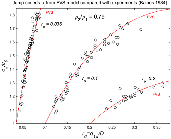
Figure 4. Comparison between jump speeds c_J (scaled with c₀) computed using the Full Vortex Sheet model (FVS) with experimental observations with water and kerosene (ρ₂/ρ₁ = 0.79), from Baines (1984).

Equations for Time-dependent Non-linear Two-layer Flow

We now consider two-layer flow over a long obstacle for which the horizontal length scale L and the time scale of the motion are sufficiently large for the equation for vertical motion to be hydrostatic, apart from the possible presence of hydraulic jumps. Under these conditions the equations of motion for the two layers may be written

$\begin{array}{ll}\frac{\partial u_1}{\partial t}+\frac{\partial }{\partial x}\left[\frac{1}{2}{u}_1^2+g\left(h+d_1+\frac{{\rho }_2}{{\rho }_1}{d}_2\right)+\frac{p_s}{{\rho }_1}\right]=0,& \left(3.1\right)\hfill \end{array}$

$\begin{array}{ll}\frac{\partial u_2}{\partial t}+\frac{\partial }{\partial x}\left[\frac{1}{2}{u}_2^2+g\left(h+d_1+d_2\right)+\frac{p_s}{{\rho }_2}\right]=0,& \left(3.2\right)\hfill \end{array}$

where u₁, u₂, d₁, d₂ denote the velocities and thicknesses of layers 1 and 2, and h(x) is the height of any bottom topography on the lower surface. If the upper layer has a rigid upper surface, and we assume that the total flow of fluid through the system is constant, we have, at all locations x,

$\begin{array}{ll}h(x)+d_1+d_2=D,d_1{u}_1+d_2{u}_2=Q,& \left(3.3\right)\hfill \end{array}$

where Q is the nett volume flux through the system, presumed constant after some initial starting time t = t₀. This system of equations governs the internal or baroclinic mode, and may be reduced to two equations for two convenient perturbation variables v and η, defined by

$\begin{array}{ll}v=u_1-\frac{{\rho }_2}{{\rho }_1}{u}_2,d_1+h=d_{10}+\eta ,d_2=d_{20}-\eta ,& \left(3.4\right)\hfill \end{array}$

where d₁₀ and d₂₀ denote a reference state for the thicknesses d₁ and d₂. If the unknown surface pressure p_s is eliminated by subtraction, from the above we may obtain equations for v and η in the form

$\begin{array}{ll}\frac{\partial \eta }{\partial t}+\frac{\partial }{\partial x}\left[\frac{\left(d_{20}-\eta \right)\left(d_{10}-h+\eta \right)v+\frac{1}{2}Q\left(\eta -d_{20}+\frac{{\rho }_2}{{\rho }_1}\left(d_{10}-h+\eta \right)\right)}{D-h-\delta }\right]=0,& \left(3.5\right)\hfill \end{array}$

$\begin{array}{ll}\frac{\partial v}{\partial t}+\frac{\partial }{\partial x}\left[\frac{\Delta \rho g\eta }{{\rho }_1}+\frac{\left[{\left(d_{20}-\eta \right)}^2-\frac{{\rho }_2}{{\rho }_1}{\left(d_{10}-h+\eta \right)}^2\right]v^2+\frac{{\rho }_2}{{\rho }_1}\left[2Qv(D-h)-\left(1-\frac{{\rho }_2}{{\rho }_1}\right)Q^2\right]}{2{(D-h-\delta )}^2}\right]=0,& \left(3.6\right)\hfill \end{array}$

where

$\begin{array}{ll}\delta =\frac{\Delta \rho }{{\rho }_1}\left(d_{10}-h+\eta \right).& \left(3.7\right)\hfill \end{array}$

These equations describe time-dependent motions in this two-layer system, which involve waves on the interface. There are two waves, propagating in opposite directions relative to the mean motion of the local fluid, and these waves may be described by the characteristic equations as follows (e.g., Whitham, 1974).

Equations (3.6–7) may be expressed as

$\begin{array}{ll}\frac{\partial \eta }{\partial t}+a_{11}\frac{\partial \eta }{\partial x}+a_{12}\frac{\partial v}{\partial x}=b_1\frac{\partial h}{\partial x},\frac{\partial v}{\partial t}+a_{21}\frac{\partial \eta }{\partial x}+a_{22}\frac{\partial v}{\partial x}=b_2\frac{\partial h}{\partial x},& \left(3.8\right)\hfill \end{array}$

where a₁₁(η, v) etc. are given in the Appendix, and in the region where h = 0, we may (trivially) write, for any arbitrary factors l₁, l₂,

$\begin{array}{ll}{l}_1\left(\frac{\partial \eta }{\partial t}+a_{11}\frac{\partial \eta }{\partial x}+a_{12}\frac{\partial v}{\partial x}\right)=0,l_2\left(\frac{\partial v}{\partial t}+a_{21}\frac{\partial \eta }{\partial x}+a_{22}\frac{\partial v}{\partial x}\right)=0.& \left(3.9\right)\hfill \end{array}$

If we may write

$\begin{array}{l}{l}_1{a}_{11}+l_2{a}_{21}=l_{1}c,l_1{a}_{12}+l_2{a}_{22}=l_{2}c,\text{which requires}\\ \text{det}\left[a_{ij}-cI\right]=0,& \left(3.10\right)\hfill \end{array}$

for real values of c, adding the two equations in Equation (3.9) gives

$\begin{array}{ll}{l}_1\left(\frac{\partial \eta }{\partial t}+c\frac{\partial \eta }{\partial x}\right)+l_2\left(\frac{\partial v}{\partial t}+c\frac{\partial v}{\partial x}\right)=0,i.e.,l_1\frac{\text{d}\eta }{\text{d}t}+l_2\frac{\text{d}v}{\text{d}t}=0,& \left(3.11\right)\hfill \end{array}$

where

$\begin{array}{ll}\frac{\text{d}}{\text{d}t}\left(\eta ,v\right)=\frac{\partial }{\partial t}\left(\eta ,v\right)+c\frac{\partial }{\partial x}\left(\eta ,v\right).& \left(3.12\right)\hfill \end{array}$

There are two solutions for c, denoted c₊ and c₋, for waves propagating rightward (with the stream c₊), and leftward, against it (c₋). It follows that the time-dependent motion at a given point is the sum of the leftward- and rightward-propagating motions with speeds given by Equation (3.10), which are

$\begin{array}{ll}{c}_{+},c_{-}=\frac{1}{2}\left(a_{11}+a_{22}\right)\pm \frac{1}{2}{\left[{\left(a_{11}-a_{22}\right)}^2+4a_{21}{a}_{12}\right]}^{1∕2}.& \left(3.13\right)\hfill \end{array}$

Two-layer Flow Over a Single Obstacle

We consider motions governed by the above equations, with the initial conditions:

$\begin{array}{ll}{u}_1=u_2=U,d_1=d_{10}+h(x),d_2=d_{20}-h(x),att=0,& \left(4.1\right)\hfill \end{array}$

after which U and h(x) remain constant. This corresponds to the sudden introduction of the obstacle into a uniform two-layer stream (the result is similar to that for the sudden onset of a uniform two-layer stream over a stationary obstacle). Our objective is to describe the properties of the resulting flow in terms of the parameters given in Equation (1.1).

For a sufficiently small obstacle, the commencement of conditions Equation (4.1) causes two transient disturbances, each having the form of the topography. One of these propagates against the flow, and the other with it, as described in Section Equations for Time-Dependent Non-linear Two-layer Flow, leaving a locally steady solution in the vicinity of the obstacle. This steady solution is given by steady forms of Equations (3.5) and (3.6), where the square-bracket terms are equal to their values where h, η, and v = 0. They may also be manipulated to give the “hydraulic alternative,” namely that

$\begin{array}{ll}\frac{\text{d}}{\text{d}x}\left(\eta ,v\right)=0,\text{or }{c}_{-}=0,\text{where}\frac{\text{d}h}{\text{d}x}=0.& \left(4.2\right)\hfill \end{array}$

If c₋ < 0 the flow is subcritical, and if both c₊, c₋ > 0 the flow is supercritical, and the steady solution applies provided c₋ ≠ 0, which implies F₀ ≠ 1.

For subcritical flows where r_u = d₁₀∕D is small, as H_m is increased the steady solution is valid until a point is reached at which c₋ = 0 at the peak of the obstacle, i.e.,

$\begin{array}{ll}{c}_{-}=\frac{1}{2}\left(a_{11}+a_{22}\right)-\frac{1}{2}{\left[{\left(a_{11}-a_{22}\right)}^2+4a_{21}{a}_{12}\right]}^{1∕2},& \left(4.3\right)\hfill \end{array}$

where a_ij are given in the Appendix with

$\begin{array}{ll}{d}_1=d_{11},d_2=d_{21},\eta ={\eta }_c,v=v_c,h=h_m,& \left(4.4\right)\hfill \end{array}$

η_c and v_c denoting the values of η and v at the critical section at the peak of the obstacle.

For larger heights the steady solution is not valid, and the fluid responds by sending a disturbance upstream, which effectively alters the upstream flow conditions. The flow over the obstacle is then no longer symmetric about the highest point, and for the resulting steady flow, the fluid must adjust so that the second alternative—c₋ = 0 applies there. Further increases in the obstacle height beyond this point cause yet faster disturbances to propagate upstream, with the result that the flow forms upstream hydraulic jumps. When this happens, it is necessary to take into account the properties of hydraulic jumps, and assuming steady flow over the obstacle, to link this to the condition c₋ = 0 at the obstacle crest. The appropriate variables and notation are shown in Figure 5. The new (correct) formulation for hydraulic jumps described in Section Hydraulic Jumps in Two-layer Flows above is used here. The simplest procedure is to assume a given upstream jump height, and then take the conditions downstream of the jump as input to flow over the topography, where the critical condition at the obstacle crest together with the steady-state forms of Equations (3.5) and (3.6) determines the obstacle height. From this one may construct regions of the F₀–H_m diagram. For subcritical flows with small r_u, the above phenomena are sufficient to describe the upstream flow properties up to the point where the lower layer becomes blocked by the topography, and is locally absent on the downstream side.

FIGURE 5

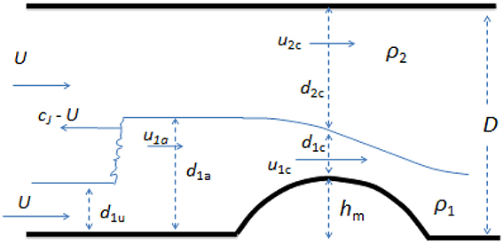
Figure 5. Definition sketch for notation for flow over an obstacle with an upstream jump. All velocities are relative to a frame of reference at rest with the obstacle. Here the velocities and thickness immediately downstream of the jump (section “a”) are the same as those immediately upstream of the obstacle.

The above procedure is essentially the same as that for single-layer flows over obstacles (e.g., Baines, 1995, 1998, Section 2.3). But for larger values of r_u, and supercritical flows, increasing H_m may cause the upstream jump to reach its maximum speed. At this point, the flow immediately downstream of the upstream jump becomes supercritical, as described in Section Hydraulic Jumps in Two-layer Flows. This means that, although larger-amplitude jumps are theoretically possible, they cannot be built up by disturbances approaching it from the downstream side, and hence the flow must respond in some other way. Increasing H_m causes more upstream disturbances that increase the lower layer thickness and progressively travel more slowly, so that the resulting upstream disturbance becomes more spread out as it propagates, rather than steepening to form an hydraulic jump. Such a disturbance is termed a rarefaction, because the disturbance itself is becoming more rarefied with time (see Chapter 3 of Baines, 1995, 1998). The resulting upstream motions are governed by Equations (3.8–12), and the flow has the form shown in Figure 6. The flow eventually reaches a quasi-steady form, with the distance between the jump and the obstacle progressively increasing, but with a dynamical link between them manifested in the interfacial waves. The only way the jump can influence the flow downstream is via the rightward-propagating waves (with speed c₊).

FIGURE 6

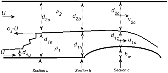
Figure 6. The same as Figure 5, except for larger obstacle heights where the flow contains a rarefaction. Here the jump has the maximum speed, and section “b” immediately upstream of the obstacle has larger lower-layer thickness than section “a,” immediately downstream of the jump.

The rightward propagating waves commence with the conditions at section a of Figure 6, immediately downstream of the jump. With c = c₊, Equation (3.11) provides the relation

$\begin{array}{ll}\frac{\text{d}v}{\text{d}\eta }=-\frac{l_1}{l_2}=-\frac{a_{11}-a_{22}\pm {\left[{\left(a_{11}-a_{22}\right)}^2+4a_{21}{a}_{12}\right]}^{1∕2}}{2a_{12}},& \left(4.5\right)\hfill \end{array}$

where the plus sign is taken. This gives a relation between v and η for these downstream propagating waves. The expressions for a₁₁(η, v) etc. are those given in the Appendix, with d₁ = d₁₁, d₂ = d₂₁, and the initial conditions of section a:

$\begin{array}{ll}\eta =0,v=u_{11}-\frac{{\rho }_2}{{\rho }_1}{u}_{21},& \left(4.6\right)\hfill \end{array}$

where u₁₁, u₂₁ are the velocities at Section Introduction in the frame of the obstacle, and are determined by the properties of the jump. Integrating Equation (4.3) then gives a relation between v and η that applies up to section b of Figure 6, immediately upstream of the obstacle.

The jump equations give the conditions (v and η) downstream of the jump at section a, and Equation (4.3) links these conditions with those upstream of the obstacle at section b. The steady-state forms of Equations (3.5) and (3.6) and the critical condition at the obstacle crest then give the obstacle height, as before. For clarity, we here describe this process in a little more detail.

In general, Equation (4.3) must be integrated numerically using the expressions in the Appendix, where d₁, d₂ denote the layer thicknesses immediately downstream of the jump. In the notation of Figure 5, the initial conditions at section a are therefore

$\begin{array}{ll}{d}_1=d_{1a},d_2=d_{2a},{\eta }_a=0,v_a=u_{1a}-\frac{{\rho }_2}{{\rho }_1}{u}_{2a},& \left(4.7\right)\hfill \end{array}$

and Equation (4.5) gives a relationship between v and η. It should be noted that Section Introduction is not at a fixed location, but the velocities in Equation (4.7) are relative to the reference frame of the obstacle, as in Figure 5.

In the Boussinesq limit, the a_ij take the form

$\begin{array}{l}{a}_{11}=\frac{v\left(d_2-d_1+h-2\eta \right)+Q}{D-h},\\ a_{12}=\frac{\left(d_2-\eta \right)\left(d_1-h+\eta \right)}{D-h},(\text{A}.11)\\ a_{21}=\frac{\Delta \rho g}{{\rho }_1}-\frac{v^2}{D-h},a_{22}=a_{11},(\text{A}.12)\end{array}$

so that Equation (4.5) can be expressed as

$\begin{array}{l}\frac{\text{d}v}{\text{d}\eta }=-{\left(\frac{a_{21}}{a_{12}}\right)}^{1∕2}=-{\left(\frac{g\prime D-v^2}{\left(d_{2a}-\eta \right)\left(d_{1a}+\eta \right)}\right)}^{1∕2},\\ \text{where }g\prime =\frac{\Delta \rho g}{{\rho }_0}.& \left(4.8\right)\hfill \end{array}$

Equation (4.8) can then be integrated directly to give the “Riemann invariant”

$\begin{array}{l}\text{arcsin}\left(\frac{2\eta +d_{1a}-d_{2a}}{D}\right)+\text{arcsin}\left(\frac{v}{{\left(g\prime D\right)}^{1∕2}}\right)\\ =\text{arcsin}\left(\frac{d_{1a}-d_{2a}}{D}\right)+\text{arcsin}\left(\frac{u_{1a}-u_{2a}}{{\left(g\prime D\right)}^{1∕2}}\right).& \left(4.9\right)\hfill \end{array}$

This gives a relationship between v and η that applies immediately upstream of the topography (denoted section b in Figure 5, with variables d_1b, d_2b, u_1b, u_2b, η_b, v_b). The flow over the obstacle may be assumed to be steady after sufficient time has elapsed. We may therefore use the steady-state versions of Equations (3.5) and (3.6) to link the flow immediately upstream of the obstacle to the flow at the obstacle crest (denoted section c in Figure 5), which for the general case give.

$\begin{array}{l}\frac{\left(d_{2a}-{\eta }_b\right)\left(d_{1a}+{\eta }_b\right)v_b+\frac{1}{2}Q\left({\eta }_b-d_{2a}+\frac{{\rho }_2}{{\rho }_1}\left(d_{1a}+{\eta }_b\right)\right)}{D-{\delta }_b}=\\ \frac{\left(d_{2a}-{\eta }_c\right)\left(d_{1a}-h_m+{\eta }_c\right)v_c+\frac{1}{2}Q\left({\eta }_c-d_{2a}+\frac{{\rho }_2}{{\rho }_1}\left(d_{1a}-h_m+{\eta }_c\right)\right)}{D-h_m-{\delta }_c},& \left(4.10\right)\hfill \end{array}$

$\begin{array}{l}g\prime {\eta }_b+\frac{\left[{\left(d_{2a}-{\eta }_b\right)}^2-\frac{{\rho }_2}{{\rho }_1}{\left(d_{1a}+{\eta }_b\right)}^2\right]v_b^2+\frac{{\rho }_2}{{\rho }_1}\left[2Q{v}_{b}D-\left(1-\frac{{\rho }_2}{{\rho }_1}\right)Q^2\right]}{2{(D-{\delta }_b)}^2}=\\ g\prime {\eta }_c+\frac{\left[{\left(d_{2a}-{\eta }_c\right)}^2-\frac{{\rho }_2}{{\rho }_1}{\left(d_{1a}-h_m+{\eta }_c\right)}^2\right]v_c^2+\frac{{\rho }_2}{{\rho }_1}\left[2Q{v}_c(D-h_m)-\left(1-\frac{{\rho }_2}{{\rho }_1}\right)Q^2\right]}{2{(D-h_m-{\delta }_c)}^2},& \left(4.11\right)\hfill \end{array}$

$\begin{array}{ll}\text{where }{\delta }_b=\frac{\Delta \rho }{{\rho }_1}\left(d_{1a}+{\eta }_b\right),{\delta }_c=\frac{\Delta \rho }{{\rho }_1}\left(d_{1a}-h_m+{\eta }_c\right).& \left(4.12\right)\hfill \end{array}$

The other remaining equation is the critical condition at the obstacle crest, as in Equation (4.3), which takes the form

$\begin{array}{l}{c}_{-}=\frac{1}{2}\left(a_{11}\left({\eta }_c,v_c,h_m\right)+a_{22}\left({\eta }_c,v_c,h_m\right)\right)\\ -\frac{1}{2}[{\left(a_{11}\left({\eta }_c,v_c,h_m\right)-a_{22}\left({\eta }_c,v_c,h_m\right)\right)}^2\\ {+4a_{21}\left({\eta }_c,v_c,h_m\right)a_{12}\left({\eta }_c,v_c,h_m\right)]}^{1/2}=0,& \left(4.13\right)\hfill \end{array}$

using the expressions for a_ij in the Appendix, with d₁ = d_1a, d₂ = d_2a. We therefore have four equations for the four variables η_b, v_b, η_c, v_c, for an upstream jump of given amplitude and hence known values of d_1a, d_2a, u_1a, u_2a, v_a, (with η_a = 0) which enables us to determine the appropriate value of h_m. Hence one may construct diagrams of flow properties in the F₀ − H_m plane, for various values of the density ratio ρ₂∕ρ₁. For the situations analyzed for this paper (shown in Figures 9, 10), the regions in F₀ − H_m space where rarefactions occur are small.

Results

With the above analysis, we may determine the nature of the two-layer flow over an obstacle, and its variation with the relevant parameters. We are concerned with flows that are (or are equivalent to being) started from a state of rest, and after a short starting period are maintained at constant conditions. This includes, for example, an obstacle that is towed through stationary fluid, or a stationary obstacle situated in a two-layer stream where the latter is suddenly forced into uniform motion.

An effective way of getting an overall view of the types of flow that may occur is through the F₀–H_m diagram. Here, given uniform initial flow velocity, we have two additional parameters: r_u = d₁₀/D, the initial relative thickness of the lower layer, and ρ₂∕ρ₁, the ratio of the densities of the fluids in the two layers. We present some representative examples of such diagrams which indicate some surprising and novel features of the flow of two fluids. This includes the phenomenon of “hysteresis,” or multiple steady flow states, in parameter ranges that include the state of fully supercritical flow over the obstacle.

As a point of reference and subsequent comparison, Figure 7 shows the F₀–H_m diagram for a single homogeneous fluid layer (from Baines and Davies, 1980; Baines, 1995, 1998). This shows parameter ranges where the ultimate steady flow is wholly subcritical or supercritical over the obstacle, where the fluid is blocked by the topography, and where the flow over the obstacle forces an upstream jump that alters the approaching flow, which is governed by a critical condition at the crest of the obstacle. There is also a parameter range within which a hysteresis phenomenon may occur. Here the flow over the obstacle may be entirely supercritical, or partially blocked (with an upstream hydraulic jump) with critical flow at the crest: subcritical on the upstream side, and supercritical on the downstream side. Which of these two states occurs in practice will depend on how the flow is set up. One may then make the transition from one state to the other by slowly varying the basic flow parameters F₀ and H_m in a quasi-static manner—hence the term “hysteresis.”

FIGURE 7

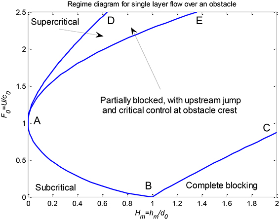
Figure 7. Regime diagram for hydrostatic single-layer flow over an obstacle. U and d₀ are the initial fluid velocity and layer thickness, with c₀ the wavespeed. In the region EABC the flow is partially blocked, with an upstream hydraulic jump controlled by a critical condition at the obstacle crest. DAE is the “hysteresis” region, in which the flow may be either partially blocked as in EABC, or supercritical, as above AD, as indicated by arrows. For more details see Section 2.3 of Baines (1995, 1998).

One may expect similar types of behavior to occur for two-layer flow over topography. Some examples have been given by Baines (1984) for the special case of water and kerosene, where a range of parameters with two states was observed experimentally. However, computations for flows in the Boussinesq limit (Baines, 1995, 1998) using the Yih-Guha hydraulic jump model (which seemed to be the best available at the time) did not give any multiple states. Here we present two parameter diagrams in which r_u = 0.1, and is representative of thin lower layers. In one of these, ρ₂∕ρ₁ is small (0.1), and in the other, 0.99, which is very close to the Boussinesq limit. The contrast between these two cases is surprising and instructive. But first, Figure 8 shows the curves for the boundary of wholly subcritical (for F₀ < 1) or wholly supercritical (for F₀ > 1) flow as the obstacle height is increased from zero in a stream with given F₀, for a range of density ratios, for r_u = 0.1. The positions and shapes of these curves are generally similar in form to that for a single layer, which is curve BAE in Figure 7. The main difference is that single-layer curve BAE is unlimited, whereas all the two-layer curves must necessarily terminate.

FIGURE 8

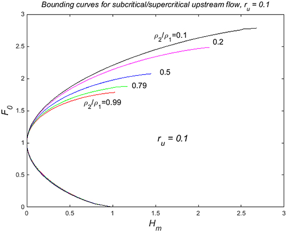
Figure 8. Curves for the onset of critical flow at the obstacle crest as H_m increases from zero, with no upstream jump, for a range of density ratios, for r_u = 0.1. For F₀ values larger (or H_m less) than those on the upper part of these curves, the steady flow is everywhere supercritical, and for F₀ (or H_m) less than the lower part (where these curves effectively coincide), the steady flow is subcritical.

Figure 9 shows the F₀ − H_m diagram for r = r_u = 0.1, ρ₂∕ρ₁ = 0.99, near the Boussinesq limit. Here curve BAE denotes the critical flow condition, with subcritical/supercritical flow to the left if F₀ < 1/F₀ > 1, and partially blocked lower-layer flow with an upstream jump to the right (as in Figure 7). The magnitude of this jump is given by the plotted values of r_a = d_1a/D. This part of the diagram extends to the line where r_a = 0.385, which is the value for the maximum jump speed. The curves terminate at the boundary where the lower layer is completely blocked, and for larger F₀, there is a small region where larger upstream motions occur through rarefactions. This is limited by the flow immediately upstream of the obstacle becoming critical, which occurs where r_b is very close to 0.45. For larger values of F₀, or H_m, the flow over the obstacle is supercritical.

FIGURE 9

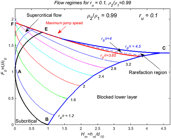
Figure 9. Flow properties for steady-state flow over an obstacle, depicted on the F₀–H_m diagram for r = r_u = 0.1, ρ₂∕ρ₁ = 0.99—the near-Boussinesq case. The flow is subcritical below AB, and upstream hydraulic jumps occur to the right of EAB below EC; the lower layer is completely blocked to the right of BC. Rarefactions that increase the upstream disturbance above that due to the jump of maximum speed occur in the small region immediately below EC, above the curve with r_a/r_u = 3.85. In the region AEFA, there are three possible flow states: supercritical flow, and two states with different upstream jump heights, given by the cross-over of the two curves passing through any given point.

This figure is similar to Figure 3.12a of (Baines, 1995, 1998), which uses Yih and Guha, as described above except that the curves for the amplitudes of upstream jumps extend beyond AE. Here, because some of these curves “double back” after touching H_m = 0, there are two additional solutions for the upstream flow, in the region below the curve for maximum jump speed. Given that the flow in this region may also be supercritical, there are three possible solutions in the region AEF—a jump at small amplitude, a jump at somewhat larger amplitude, and no jump at all (supercritical flow, as indicated by the arrow). It is possible that one or more of these jumps may be unstable, but this has not been investigated.

The F₀ − H_m diagram for r = 0.1, ρ₂∕ρ₁ = 0.1 is shown in Figure 10. Here the overall pattern is the same as for Figure 9, with the exception that the bounding curve BADE for supercritical flow extends above the boundary line FDC for partially blocked flows. In particular there is a region above FD where partially blocked or completely supercritical flows are possible, between DE and the axis H_m = 0. This is an upward extension of the curves that commence from the line BC. Hence, there are six different regions in this diagram. The first four are: subcritical flow below AB, blocked lower layer below BC, supercritical flow above GEDC, and partially blocked flow with upstream jump in DABCD; in these regions the flow state for given (F₀, H_m) is unique. In the region ADFA there are three possible flow states: supercritical flow, and two possible critically controlled flows with different upstream jumps, given by the intersecting contours of jump height at any particular point. In section DEGFD the same applies, except that there is only one possible upstream jump. This latter region is curious because, when compared with the diagram for single-layer flows (Figure 7), the region with multiple states is to the left of curve ADE, whereas for single-layer flows it is to the right of it.

FIGURE 10

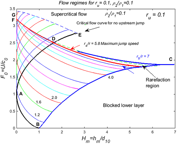
Figure 10. As for Figure 9, but for the parameters r_u = 0.1, ρ₂∕ρ₁ = 0.1. The properties are essentially the same, except for the region DEGF, within which the flow has two possible flow states: supercritical flow, or critical flow at the obstacle crest with an upstream jump.

A corresponding diagram for r_u = 0.1, ρ₂∕ρ₁ = 0.5 (not shown) displays the same features as in Figure 10, but the region ADFA is less pronounced, so that the diagram is closer to that of Figure 9, as might be expected.

Conclusions

We have used a new (and within its limitations, essentially correct) formulation of two-layer hydraulic jumps to determine the properties of non-linear flow over long obstacles. This hydraulic jump formulation uses a vorticity balance to infer the pressure differences across the jump, and avoids assumptions made in earlier models that are now seen to be incorrect. The model can be (and has been) applied to a full range of upstream conditions and density ratios, and hence is not restricted to the Boussinesq limit. For obstacles moving relative to fluid at rest, there are four main dimensionless parameters involved: the lower layer thickness ratio r_u = d₁₀/D, the density ratio ρ₂∕ρ₁, the initial Froude number F₀, and the obstacle height ratio H_m = h_m/d₁₀.

The nature of the resulting flows (steady over the obstacle) has features similar to those obtained with a single layer—sub- or supercritical flow for small obstacle heights for small values of H_m, and an upstream hydraulic jump followed by a thicker lower layer and governed by a critical condition at the obstacle crest, for larger H_m. The hydraulic jumps, however, have a maximum speed, and when this is reached, larger amplitude jumps cannot be forced from the topography. Instead, the upstream disturbances forced by larger obstacle heights have the form of rarefactions, which become elongated and lag behind the jump. For r_u values ≥0.5, only rarefactions are present, and previous analysis without jumps is still valid (e.g., Figure 3.12d of Baines, 1995, 1998).

The use of the new hydraulic jump formulation produces some surprises that are best seen in the flow types in the various regions of the F₀-H_m plane diagrams of Figures 9, 10. These are very different from previous versions (see for example Figures 3.12a,b of Baines, 1995, 1998) which used the jump formulation of Yih and Guha (1955). Figure 9 shows results for ρ₂∕ρ₁ = 0.99, near the Boussinesq limit. Here the surprise is in the “supercritical” region AEF, where in addition to possibly being supercritical, the flow may have two other flow states with upstream jumps, of different heights. In Figure 10, the same phenomenon is seen in region ADF, but now there is an additional region FDEG in which there are two possible states—supercritical flow, or an upstream jump with critical flow at the crest. This region FDEG is vanishingly small for ρ₂∕ρ₁ = 0.99, but increases in size as ρ₂∕ρ₁ decreases toward zero.

Author Contributions

This work relies heavily on earlier work by PGB who initiated the present study. ERJ contributed subsequently. Both authors approved it for publication.

Conflict of Interest Statement

The authors declare that the research was conducted in the absence of any commercial or financial relationships that could be construed as a potential conflict of interest.

References

Baines, P. G., and Davies, P. A. (1980). “Laboratory studies of topographic effects in rotating and/or stratified fluids,” in Orographic Effects in Planetary Flows, GARP Publication No. 23 (World Meteorological Organisation/Ingernational Council of Scientific Unions), 233–299.

Google Scholar

Baines, P. G. (1984). A unified description of two-layer flow over topography. J. Fluid Mech. 146, 127–167.

Google Scholar

Baines, P. G. (1995, 1998). Topographic Effects in Stratified Flows. Cambridge, UK: Cambridge University Press.

Baines, P. G. (2015). Internal hydraulic jumps in two-layer systems. J. Fluid Mech. 787, 1–15. doi: 10.1017/jfm.2015.662

CrossRef Full Text | Google Scholar

Borden, Z., and Meiburg, E. (2013). Circulation-based models of Boussinesq internal bores. J. Fluid Mech. 276, R1, doi: 10.1017/jfm.2013.239

CrossRef Full Text | Google Scholar

Chu, V. H., and Baddour, R. E. (1977). Surges, waves and mixing in two-layer density stratified flow. Proc. Int. Assn. Hydraul. Res. 1, 303–310.

Klemp, J. B., Rotunno, R., and Skamarock, W. C. (1997). On the propagation of internal bores. J. Fluid Mech. 331, 81–106.

Google Scholar

Li, M., and Cummins, P. F. (1998). A note on hydraulic theory of internal bores. Dyn. Atmos. Oceans 28, 1–7.

Google Scholar

White, B. L., and Helfrich, K. R. (2014). A model for internal bores in continuous stratification. J. Fluid Mech. 761, 282–304. doi: 10.1017/jfm.2014.599

CrossRef Full Text | Google Scholar

Whitham, G. B. (1974). Linear and Non-Linear Waves. New York, NY: J. Wiley & Sons. 636.

Wood, I. R., and Simpson, J. E. (1984). Jumps in layered miscible fluids. J. Fluid Mech. 140, 329–342.

Google Scholar

Yih, C.-S., and Guha, C. R. (1955). Hydraulic jump in a uid system of two layers. Tellus 7, 358–366.

Google Scholar

Appendix

The functions a_ij, b_i in Equation (3.8) take the following general forms. The variable η is relative to layer thicknesses d₁, d₂, for the lower and upper layers respectively, where d₁ + d₂ + h = D. With d₁ and d₂ as reference values, for a_ij(η, v) we have

$\begin{array}{ll}{a}_{11}=\frac{v\left(d_2-d_1+h-2\eta \right)+\frac{Q}{2}\left(1+\frac{{\rho }_2}{{\rho }_1}\right)}{D-h-\delta }+\frac{\Delta \rho }{{\rho }_1}\frac{T_1}{{\left(D-h-\delta \right)}^2},& \left(\mathrm{A1}\right)\hfill \end{array}$

where

$\begin{array}{l}{T}_1=v\left(d_2-\eta \right)\left(d_1-h+\eta \right)\\ +\frac{Q}{2}\left(\eta -d_2+\frac{{\rho }_2}{{\rho }_1}\left(d_1-h+\eta \right)\right),\\ \delta =\frac{\Delta \rho }{{\rho }_1}\left(d_1-h+\eta \right),& \left(\mathrm{A2}\right)\hfill \end{array}$

$\begin{array}{ll}{a}_{12}=\frac{\left(d_2-\eta \right)\left(d_1-h+\eta \right)}{D-h-\delta },& \left(\mathrm{A3}\right)\hfill \end{array}$

$\begin{array}{ll}{a}_{21}=\frac{\Delta \rho g}{{\rho }_1}-\frac{v^2\left(d_2-\eta +\frac{{\rho }_2}{{\rho }_1}\left(d_1-h+\eta \right)\right)}{{\left(D-h-\delta \right)}^2}+\frac{\Delta \rho }{{\rho }_1}\frac{T_2}{{\left(D-h-\delta \right)}^3},& \left(\mathrm{A4}\right)\hfill \end{array}$

where

$\begin{array}{l}{T}_2=v^2\left[{\left(d_2-\eta \right)}^2-\frac{{\rho }_2}{{\rho }_1}{\left(d_1-h+\eta \right)}^2\right]\\ +\frac{{\rho }_2}{{\rho }_1}Q\left(2vD-\left(1-\frac{{\rho }_2}{{\rho }_1}\right)Q\right),& \left(\mathrm{A5}\right)\hfill \end{array}$

$\begin{array}{ll}{a}_{22}=\frac{\left[v\left({\left(d_2-\eta \right)}^2-\frac{{\rho }_2}{{\rho }_1}{\left(d_1-h+\eta \right)}^2\right)+\frac{{\rho }_2}{{\rho }_1}Q(D-h)\right]}{{(D-h-\delta )}^2}.& \left(\mathrm{A6}\right)\hfill \end{array}$

If one can make the assumption

$\begin{array}{ll}\eta \frac{\Delta \rho }{{\rho }_1}<<D-\frac{\Delta \rho }{{\rho }_1}{d}_1-h\left(1-\frac{\Delta \rho }{{\rho }_1}\right),(A.7)& \left(\mathrm{A7}\right)\hfill \end{array}$

which implies $\delta \approx \frac{\Delta \rho }{{\rho }_1}\left(d_1-h\right)$, and if h = 0, these reduce to

$\begin{array}{ll}\eta \frac{\Delta \rho }{{\rho }_1}<<D-\frac{\Delta \rho }{{\rho }_1}{d}_1,\text{and }\delta \approx \frac{\Delta \rho }{{\rho }_1}{d}_1,(A.8)& \left(\mathrm{A8}\right)\hfill \end{array}$

the above expressions simplify to

$\begin{array}{l}{a}_{11}=\frac{v\left(d_2-d_1+h-2\eta \right)+\frac{Q}{2}\left(1+\frac{{\rho }_2}{{\rho }_1}\right)}{D-h-\delta },\\ a_{12}=\frac{\left(d_2-\eta \right)\left(d_1-h+\eta \right)}{D-h-\delta },& \left(\mathrm{A9}\right)\hfill \end{array}$

$\begin{array}{l}{a}_{21}=\frac{\Delta \rho g}{{\rho }_1}-\frac{v^2\left(d_2-\eta +\frac{{\rho }_2}{{\rho }_1}\left(d_1-h+\eta \right)\right)}{{\left(D-h-\delta \right)}^2},\\ a_{22}=\frac{\left[v\left({\left(d_2-\eta \right)}^2-\frac{{\rho }_2}{{\rho }_1}{\left(d_1-h+\eta \right)}^2\right)+\frac{{\rho }_2}{{\rho }_1}Q(D-h)\right]}{{(D-h-\delta )}^2},& \left(\mathrm{A10}\right)\hfill \end{array}$

If we further make the Boussinesq approximation (ρ₂ = ρ₁, except for the first term in a₂₁) we have

$\begin{array}{l}{a}_{11}=\frac{v\left(d_2-d_1+h-2\eta \right)+Q}{D-h},\\ a_{12}=\frac{\left(d_2-\eta \right)\left(d_1-h+\eta \right)}{D-h},& \left(\mathrm{A11}\right)\hfill \end{array}$

$\begin{array}{ll}{a}_{21}=\frac{\Delta \rho g}{{\rho }_1}-\frac{v^2}{D-h},a_{22}=a_{11}.& \left(\mathrm{A12}\right)\hfill \end{array}$