Constraining the Origins of the Magnetism of Lepidocrocite (γ-FeOOH): A Mössbauer and Magnetization Study

Introduction

Iron oxides and oxyhydroxides are widespread magnetic minerals in geologic records. Quantifying the magnetic assemblage of natural samples allows deciphering past geologic, environmental, climatic, pedogenic, or diagenetic conditions (e.g., Liu et al., 2012). Among these minerals, lepidocrocite (γ-FeOOH) has been less studied from a magnetism point of view than other iron-bearing minerals. It is commonly found in hydromorphic soils where there is seasonal alternation of reducing and oxidizing conditions, and has been shown to be a precursor of more magnetic phases such as maghemite or magnetite (eg., Fitzpatrick et al., 1985; Gehring and Hofmeister, 1994; Cornell and Schwertmann, 2003; Gendler et al., 2005; Till et al., 2014). Lepidocrocite is a ferric oxyhydroxide, orange in color, with an orthorhombic crystal structure (e.g., Ewing, 1935). The structural model consists of double chains of edge-sharing FeO₃(OH)₃ octahedra running along the c-axis. These double chains share edges to form layers, which are connected by hydrogen bonds (e.g., Eggleton et al., 1988). Natural and synthetic samples occur as needle shaped crystallites or platelets with one of their dimensions that can reach a few nanometers, the other two being much larger. Lepidocrocite is an antiferromagnet with a Néel temperature, T_N, ranging from 50 to 70 K depending on crystallinity and possibly water content (Johnson, 1969; De Grave et al., 1986). Although the Mössbauer spectra resemble those of an ensemble of superparamagnetic nanoparticles, it is clearly established, in particular through in-field Mössbauer spectra (De Grave et al., 1986), that lepidocrocite is paramagnetic above T_N and that the shape of the Mössbauer spectra reflects an unusually broad distribution of Néel temperatures. Another puzzling feature of lepidocrocite is that the Field Cooled (FC) and Zero Field Cooled (ZFC) branches of the low field direct current (dc) susceptibility (Lee et al., 2004) are also akin to those encountered in ensembles of superparamagnetic nanoparticles (Tronc et al., 1995), although lepidocrocite laths or needles cannot be considered, from a magnetism point of view, as nanometric particles. Hirt et al. (2002) proposed several interesting hypotheses to explain the low temperature magnetic behavior of lepidocrocite, but did not provide a definite picture. They proposed the existence of a defect moment and a rather large range of T_N-values, but observed the presence of shifted magnetic hysteresis loops below T_N and the persistence of a low temperature remanent magnetization (acquired in 2.5 T while cooling from 300 to 5 K) well above T_N during thermal demagnetization. The first observation was attributed to either a minor loop (as the maximum field was not enough to saturate the sample) or exchange bias arising from defective regions behaving like ferrimagnets, while the second observation was attributed to the presence of a small inducing field in the instrument. This persistence of a remanent magnetization at temperatures higher than T_N was also observed in other samples (Till et al., 2014), suggesting that it is inherent to lepidocrocite. Till et al. (2014) also showed that nanoparticles of maghemite formed within the larger particles of lepidocrocite, during the early stage of lepidocrocite dehydroxylation achieved through moderate heating under oxidizing conditions.

In the present study, a comprehensive interpretation of ⁵⁷Fe Mössbauer spectroscopy and magnetization (in zero, constant, or alternating field) data acquired on synthetic lepidocrocite is presented. It is demonstrated that the occurrence of two magnetic behaviors can be tracked in all measured quantities, one due to the antiferromagnetic (AFM) bulk material and the other to sparse (probably) ferrimagnetic nanoparticles similar to (but in lesser content) those observed during moderate heating of lepidocrocite. Supporting evidence is provided from modeling efforts. We discuss the possible form of this coexistence, which seems to be inherent to lepidocrocite although the concentration of ferrimagnetic nanoparticles appears to be sample dependent.

Materials and Methods

Sample Synthesis

A batch of lepidocrocite was prepared by mixing a 0.228 M solution of FeCl₂·4H₂O with a 0.4 M solution of NaOH to precipitate an Fe(II) hydroxide (Ona-Nguema et al., 2002). The resulting suspension was aerated at 25°C by continuous magnetic stirring to oxidize the precipitate, leading to a change in color of the suspension from dark green to orange. The reaction was also monitored through recording of Eh and pH values. The precipitate was subsequently removed from the suspension by centrifuging, washed with Milli-Q^® water to remove electrolytes and vacuum-dried in a desiccator. A representative transmission electron microscope (TEM) image of the resulting sample is shown in Figure 1, displaying platy particles with an approximate length of 100 nm, and irregular terminations. An X-ray diffraction (XRD) pattern of the sample was obtained using Co (Kα) radiation on a Panalytical XPert PRO MPD diffractometer, displaying all the diffraction peaks of lepidocrocite and confirming the absence of contamination (Figure 2). The lepidocrocite sample has an orthorhombic symmetry for which cell parameters are a = 3.88 Å, b = 12.60 Å and c = 3.07 Å when the space group is Vh¹⁷ – Amam. These parameters are similar to those previously obtained by Ewing (1935).

FIGURE 1

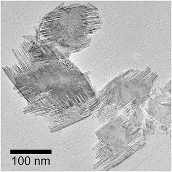
Figure 1. Transmission electron micrograph of the lepidocrocite sample.

FIGURE 2

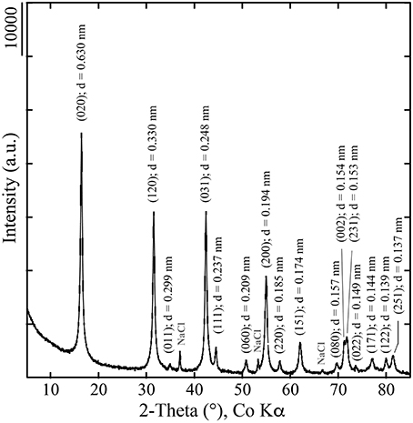
Figure 2. X-ray diffractogram of the lepidocrocite sample.

Magnetic Characterization Methods

The ⁵⁷Fe Mössbauer spectra were recorded using a constant acceleration electromagnetic drive to which is attached a ⁵⁷Co/Rh commercial γ-ray source. Spectra were obtained in the 4.2–77 K temperature range. Isothermal magnetization curves were measured on dry powder in a Cryogenic Ltd Vibrating Sample Magnetometer up to 7 T in the 10–250 K temperature range. Low field direct curent (dc) susceptibility (i.e., measured in constant magnetic field) was measured on dry powder from 10 to 300 K using a Cryogenic Ltd SQUID magnetometer, in the Zero Field Cooled (ZFC) and Field Cooled (FC) procedures. In the ZFC procedure, the sample is cooled in zero external magnetic field and the dc magnetic susceptibility measured using a 5 mT magnetic induction, while in the FC procedure the sample is cooled in a 5 mT magnetic induction prior to measurement. Alternating current (ac) susceptibility (i.e., measured in an alternating magnetic field) was measured in a Quantum Design MPMS (Magnetic Properties Measurement System) with a magnetic induction of amplitude 0.2 mT and frequencies of 1, 10, 100, and 1000 Hz. The MPMS was also used to measure the temperature variation of the isothermal remanent magnetization (IRM) imparted with a 2.5 T magnetic induction at 10 K, either after cooling the sample from 300 K in zero field (ZFC IRM) or in a 2.5 T magnetic induction (FC IRM). The zero field in the MPMS used for these experiments is better than 0.5 μT. Additionally, a Cisowski test was performed using the MPMS at 10 K (e.g., Cisowski, 1981; Moskowitz et al., 1997), which consisted in stepwise acquisition of the IRM up to 2.5 T, followed by the stepwise demagnetization using backfields exactly opposite to those used for the acquisition.

Results

⁵⁷Fe Mössbauer Spectroscopy

The Mössbauer spectra obtained at 4.2, 40, and 77 K are shown in Figure 3. These spectra are similar to those presented in De Grave et al. (1986) with a magnetic hyperfine pattern at low temperature (blue line in Figure 3) whose lines broaden and whose relative weight decreases on heating, to the profit of a paramagnetic two-line sub-spectrum (green line in Figure 3). The mean hyperfine field at 4.2 K is 44.9(1) T, close to the previously published values of 44.4 T (De Grave et al., 1986) and 46 T (Johnson, 1969). At higher temperature, the magnetic sub-spectrum was fitted to a hyperfine field histogram. The thermal variation of the relative intensity of the doublet spectrum, which corresponds to the paramagnetic fraction of the sample, is represented in Figure 4. One can define the Néel temperature (T_N) as the temperature at which half the sample is paramagnetic, which in our case leads to T_N = 46.5 K. Our lepidocrocite sample shows a broad coexistence region of about 20 K around T_N (i.e., an unusually broad distribution of Néel temperatures) that could be linked to different degrees of crystallization or different contents of excess structural water (De Grave et al., 1986) in the crystallites.

FIGURE 3

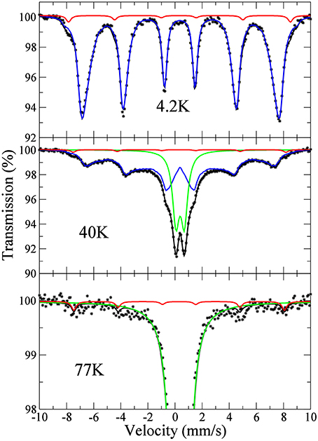
Figure 3. ⁵⁷Fe Mössbauer spectra in lepidocrocite at selected temperatures; the lines are fits and show the decomposition in sub-spectra. The close-up of the 77 K spectrum focuses on the presence of the small (red line) component

FIGURE 4

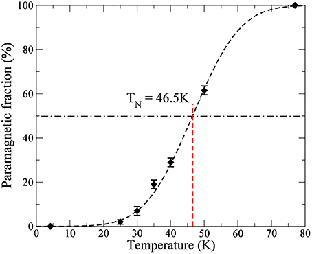
Figure 4. Thermal variation of the paramagnetic fraction (green sub-spectrum in Figure 3); the line is a fit to an erf function.

A small intensity component (red line in Figure 3) with a hyperfine field of 51.0(5) T at 4.2 K is also visible in the spectra, which is still present with a slightly decreased hyperfine field at 77 K (close-up of the 77 K spectrum in Figure 3). This small intensity component could easily be overlooked if Mössbauer spectroscopy is only conducted at room temperature. Its relative weight is estimated at 1.5(5) at.% from its relative area. Its saturated hyperfine field value matches that of ferric oxides like ferrimagnetic maghemite γ-Fe₂O₃ or oxyhydroxides like antiferromagnetic goethite α-FeOOH (e.g., Greenwood and Gibb, 1971; Murad and Cashion, 2004). As shown in several previous studies, lepidocrocite transforms to maghemite through dehydroxylation (e.g., Gehring and Hofmeister, 1994; Cudennec and Lecerf, 2005; Till et al., 2014). The presence of a small amount of maghemite in the sample would thus not be surprising.

Isothermal Magnetization

Isothermal magnetization curves are shown in Figure 5. At all temperatures, these curves show a pronounced downward curvature, which can be attributed to a Langevin-like behavior, superimposed to a variation linear with the field. This linear component is characteristic of an antiferromagnetic (AFM) structure below the spin-flip field. Its slope, referred to as χ_AFM, shows a small variation with temperature (Figure 6), with an asymptotic value of 5.34 × 10⁻⁷ m³/kg.

FIGURE 5

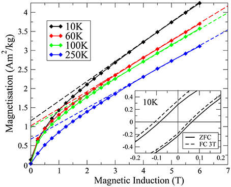
Figure 5. Isothermal magnetization curves in lepidocrocite at selected temperatures; the dashed lines are fits of the magnetization curves to a linear law: M = M₀ + χ_AFM μ₀ H. Inset: close-up of the hysteresis loop at 10 K.

FIGURE 6

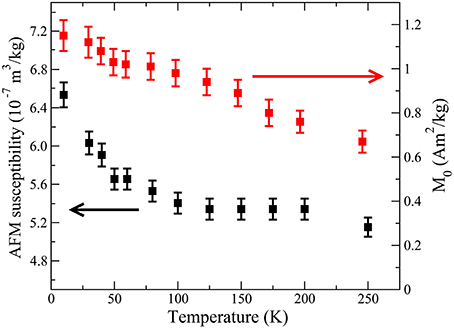
Figure 6. Thermal variations of the quantities M₀ and χ_AFM. Note that the ordinate scale for χ_AFM does not start at 0.

In the framework of a simple two-sublattice three-dimensional mean field theory, the values of χ_AFM and T_N are linked through the single ion molecular field constant λ:

$\begin{array}{l}{\chi }_{AFM}=\frac{1}{3\left|\lambda \right|}\text{ and }{T}_N=\left|\lambda \right|{\mu }_B\frac{S(S+1)}{3}{g}^2\frac{{\mu }_B}{k_B},\\ \text{with the Landé factor}g=2\text{ and spin }S=5∕2.\end{array}$

In this expression, μ_B is the Bohr magneton and k_B the Boltzmann constant. The χ_AFM-value determined for our lepidocrocite sample, 5.34 × 10⁻⁷ m³/kg, leads to T_N = 392 K. For comparison, χ_AFM in goethite is 3.96 × 10⁻⁷ m³/kg (Coey et al., 1995), which corresponds to a theoretical value of T_N = 532 K, close to the actual Néel temperature of about 400 K (e.g., Özdemir and Dunlop, 1996). In our lepidocrocite sample, the Néel temperature (ca. 50 K) obtained by Mössbauer spectroscopy is much lower than the theoretical value. Furthermore, contrary to usual antiferromagnets, the shape of the χ_AFM(T) curve does not show a clear anomaly at T_N. Both observations could be due to the bi-dimensional character of the Fe layers in this material. It has been known for a long time that the Heisenberg model for exchange interactions shows no magnetic ordering in a bi-dimensional lattice (Mermin and Wagner, 1966). Long range ordering can be restored at low temperature by (usually weak) inter-plane interactions, resulting in a reduced Néel temperature, although the in-plane exchange can be quite strong.

The intercept of the linear part of M with the ordinate axis, M₀, can be considered as the saturation magnetization of a ferrimagnetic component in lepidocrocite (Figure 5). Its value decreases on heating, more slowly above about 50 K than below, and a rough extrapolation of its thermal variation shows that it should go to zero well above room temperature (Figure 6). Identifying this component with the small intensity (1.5 at.%) phase observed in the Mössbauer spectra, the saturated M₀-value of 1.1 Am²/kg corresponds to a saturated magnetization M_s = 73 Am²/kg (assuming that lepidocrocite and the extra phase have similar Fe mass %). As it will be presented in the next section, the dc susceptibility curves show that the FC/ZFC irreversibility temperature T_irr attributed to this component is close to 80 K. Therefore, one can consider that its magnetization obeys a Langevin law above 80 K. Figure 7 shows its field variation, obtained by subtracting the linear law (χ_AFM × μ₀H) from the magnetization curves, at selected temperatures above T_irr. The lines are fits to a Langevin law with a log-normal distribution of particles with a mean diameter d₀ = 3.4 nm and a log-normal dispersion σ = 0.22, assuming a 1.5% mass fraction of the ferrimagnetic phase. For a given particle volume V, the argument of the Langevin function ${L}$(x) = 1∕tanh x − 1∕x is x = MsVH∕k_BT, resulting in a strong dependence of the curvature of the Langevin law on the mean volume <V> or mean diameter d₀ of the particles. The fit of the field variations in Figure 7 indicates that the ferrimagnetic particles are quite small, with a mean diameter d₀ = 3.4 nm. The agreement with the experimental data is quite good, the M_s(T) values corresponding to the M₀ (T) values shown in Figure 6 (M_s = M₀/0.015). Furthermore, the M/M_sat vs. B/T curves are found to superpose quite well, confirming the superparamagnetic behavior of this system. This interpretation leads us to consider that nanosized ferrimagnetic inclusions are embedded in the lepidocrocite matrix.

FIGURE 7

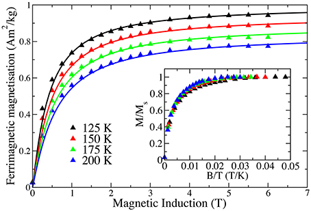
Figure 7. Ferrimagnetic contribution to the magnetization at 125, 150, 175, and 200 K; the lines are fits to a Langevin law. Inset: Normalized magnetization curves scaled with temperature.

This picture is in line with the observed hysteresis visible at 10 K (insert of Figure 5), which disappears above 30 K. The loop is slightly asymmetric, with coercive fields H${}_c^{+}=0.066$ T and H${}_c^{-}$ = −0.084 T. It is shifted along the field axis by an additional −0.020 T after field cooling under 3 T, while there is no shift of the loop along the magnetization axis. This behavior is typical of exchange-bias, a well-documented phenomenon observed in nanoparticles with a ferrimagnetic core and an antiferromagnetic outer shell (e.g., Iglesias et al., 2008), where the exchange field at the interface acts to shift the ferrimagnetic hysteresis loop. A similar observation was reported in Hirt et al. (2002), where it was attributed either to an under-saturation of the sample (and thus a minor loop was measured) or to exchange bias between the bulk of the lepidocrocite particles (antiferromagnetic) and defective regions with uncompensated spins behaving like ferrimagnets. Considering our observations based on both Mössbauer and magnetometry measurements of the coexistence of antiferromagnetism (with T_N around 46.5 K) and ferrimagnetism (with T_irr around 80 K), the observed asymmetric loop in lepidocrocite is more likely due to the exchange bias exerted by the antiferromagnetic matrix on the ferrimagnetic nano-inclusions.

dc and ac Magnetic Susceptibility

The thermal variation of the low field dc susceptibility is shown in Figure 8. The overall shape of these curves corresponds to the response of an ensemble of ferrimagnetic nanoparticles (Gittleman et al., 1974; Tronc et al., 1995) or of uncompensated antiferromagnetic particles (Gilles et al., 2000). The irreversibility temperature (T_irr) between the FC and ZFC branches is around 80–100 K and the blocking temperature (with respect to the characteristic time of the magnetic measurements, τ = 100 s) is about 50 K (maximum of the ZFC curve). The rather flat character of the FC curve below 50 K suggests the possible presence of inter-particle interactions (Tronc et al., 1995). The presence of interactions is also suggested by the Cisowski test (e.g., Cisowski, 1981; Moskowitz et al., 1997) performed at 10 K. The crossover point between the appropriately normalized IRM acquisition and demagnetization curves occurs at 0.45, close to but slightly less than the value of 0.5 expected for non-interacting systems. If one neglects these interactions as a first approximation, it is possible to simulate a ZFC curve using the formalism developed by Gittleman et al. (1974) for an ensemble of volume distributed particles. Once the mean particle diameter d₀ is known, the anisotropy density K can be deduced since the temperature of the maximum of the ZFC curve is proportional to the product $K{d}_0^3$. Identifying the susceptibility in excess of the antiferromagnetic susceptibility (taken to be 5.34 × 10⁻⁷ m³/kg) with that of the ferrimagnetic nano-inclusions, with mean diameter d₀ = 3.4 nm, and assuming a log-normal diameter distribution, we obtain a good reproduction of the ZFC curve with an anisotropy density K = 3.2 × 10⁵ J/m³ and a log-normal deviation of the diameter distribution σ = 0.22 (red curve in Figure 8). With a ferrimagnetic mass content of 1.5%, the obtained saturation magnetization of the particle M_s = 77 Am²/kg is very close to the M_s-value determined from the magnetization curves (73 Am²/kg), measured on a different instrument. We note that the deduced K-value must be considered as an estimate since the inter-particle interactions were neglected in the calculation. Therefore, the dc magnetic responses in lepidocrocite, both low field and high field, after subtraction of the AFM susceptibility of the bulk phase, correspond to those of ferrimagnetic nanoparticles of 3.4 nm mean diameter and low temperature magnetization of about 70 Am²/kg.

FIGURE 8

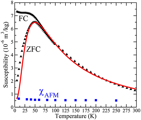
Figure 8. ZFC and FC branches of the susceptibility vs. temperature in lepidocrocite measured with a field of 5 mT and cooled with the same field in the FC procedure. The red curve is a calculation of the ZFC susceptibility using a model of independent volume distributed particles (see text). The blue points represent the AFM susceptibility

The thermal variation of the in-phase χ′ and out-of-phase χ″ components of the ac magnetic susceptibility are shown in Figure 9. Frequency dependence of the amplitude of χ′ is clearly observed from about 20 to 100 K. This region is larger than the one in the sample L89 measured by Hirt et al. (2002), where it can only be observed below 60–70 K. In Till et al. (2014), this frequency dependence was also observed in the two samples of their study. Both samples were synthesized using the same method as in the present study, the only difference being the precipitate oxidation rate. In their study, the frequency dependence in χ' was observed below about 100 K in the rapid synthesis sample and below about 150 K in the slow synthesis sample. This phenomenon thus appears to be sample dependent. Furthermore, in our sample, the temperature T_max of the maximum of χ′(T) is seen to slightly increase as frequency increases, from 54 K at 1 Hz to 60 K at 1000 Hz. This is characteristic of an ensemble of superparamagnetic particles (Dormann et al., 1997), although the T_max variation is quite small. This variation is small enough that it would not have been observed if measurements were taken every 10 K, as in previous studies (Hirt et al., 2002; Till et al., 2014). For an ensemble of non-interacting particles with a mean anisotropy barrier E_a = K <V>, the relationship between T_max and the frequency f is an Arrhenius law: f = 1/τ₀ exp(−E_a/(k_BT_max)) (Néel, 1949), where τ₀ appearing in the pre-exponential factor is τ₀ is an attempt time characteristic of the material, which should be of order 10⁻⁹–10⁻¹² s. Using this law to fit our data leads to τ₀ = 10⁻³⁵ s, which is considered to be unrealistically small and possibly due to magnetic interactions (e.g., Dormann et al., 1997). In the present case, such interactions could be dipolar in nature if locally the concentration of ferrimagnetic nano-particles was large enough. Alternatively, considering 3.4 nm diameter γ-Fe₂O₃ ferrimagnetic nanoparticles embedded in a γ-FeOOH antiferromagnetic matrix, one can expect the surface spins of the ferrimagnetic nanoparticles to be strongly dependent on the magnetic state of the lepidocrocite matrix. Magnetic exchange interactions between the antiferromagnetic matrix and the ferrimagnetic particles (as suggested by the exchange bias evidenced in Figure 5), could lead to the existence of a surface anisotropy rapidly varying when heating through T_N. In Figure 10, we compare two models of in-phase ac magnetic susceptibility, one using only the bulk anisotropy and one using a combination of bulk and surface anisotropy. Following Gittleman et al. (1974) the ac magnetic susceptibility can be written as:

$\begin{array}{l}{\chi }_{ac}=\frac{({\mu }_{0}V{M}_s^2∕3k_{B}T)+\left({\mu }_0{M}_s^2∕3K\right)i\omega \tau }{1+i\omega \tau },\\ \text{with }\omega =2\pi f\text{ and }\tau ={\tau }_0\text{exp}(KV∕k_{B}T)\end{array}$

FIGURE 9

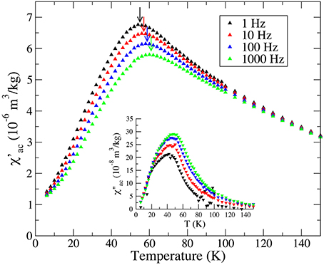
Figure 9. Low-temperature alternative current (ac) magnetic susceptibility curves (χ′). The out-of-phase magnetic susceptibility (χ″) is displayed in the inset.

FIGURE 10

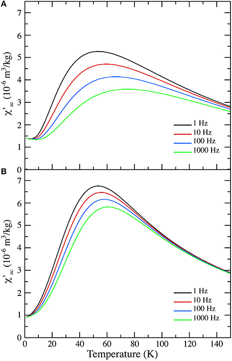
Figure 10. Models of low-temperature alternative current (ac) magnetic susceptibility curves (χ′) for 3.4 nm superparamagnetic particles with an effective anisotropy of 3.2 × 10⁵ J/m³ (A) and two component anisotropy with a volume anisotropy of 3 × 10⁴ J/m³ and a surface anisotropy of 5.1 × 10⁻⁵ J/m² (at 10 K) (B).

In these expressions, f is the alternating field frequency, τ₀ the pre-exponential time constant, M_s the saturation magnetization, μ₀ the permeability of free space, and k_B the Boltzmann constant. The magnetic anisotropy K can be taken as the bulk anisotropy value, K = K_bulk, or a combination of bulk and surface anisotropy, K = K_bulk + K_surf(S∕V), for particles of volume V and surface area S. To this expression, we added the thermal variation of χ_AFM, using a fit to the results of Figure 6. Thermal variations of M_S were also assumed to follow those depicted in Figure 6. An initial M_S-value of 75 Am²/kg was used to scale appropriately the model. The values of χ′ were calculated by taking the real part of χ_ac, after integration over the whole range of nanoparticles volumes. Figure 10A shows the results of this model using K_bulk = 3.2 × 10⁵ J/m³. As expected, the model is quite different from the measured data shown in Figure 9, as the modeled peaks are broader and their positions quite different. In Figure 10B, we used K_bulk = 3 × 10⁴ J/m³ and a thermal variation of the surface anisotropy similar to that of M_S, assuming that the surface anisotropy would be changing significantly between 0 and 50 K, as the lepidocrocite matrix would reach its Néel temperature. The initial value of K_surf was taken as 5.1 × 10⁻⁵ J/m² (at T = 0 K) and its asymptotic value as 1.2 × 10⁻⁶ J/m² (at T = 300 K). The shape of the modeled χ′ closely resemble that of the measured in-phase susceptibility, both in terms of peak shapes and positions.

Low Temperature Remanent Magnetizations

The thermal evolution of the remanent magnetizations obtained through the zero field cooling (ZFC IRM) and field cooling (FC IRM) procedures in a 2.5 T induction are displayed in Figure 11. The two curves are separated for temperatures below about 100 K, which implies that a 2.5 T magnetic induction applied at 10 K is not sufficient to magnetize the sample after cooling in zero field. Such phenomenon has been observed in previous studies on lepidocrocite (Hirt et al., 2002; Till et al., 2014), although the temperature at which the FC and ZFC IRM curves merge is different. In the study by Hirt et al. (2002), the ZFC and FC IRM curves of their pure lepidocrocite sample L89 merge at 250 K. In Till et al. (2014), the curves merge at 100 and 150 K for the slow and rapid syntheses, respectively. This can be attributed to differences in the size distribution of the ferrimagnetic regions, which are likely to be sample dependent. Unblocking of the magnetization is rather rapid at low-temperature, reflecting what was already observed in the FC/ZFC dc susceptibility measurements. For comparison, the difference between FC and ZFC dc susceptibility data (Figure 8), normalized by the value at 10 K, is represented in the inset of Figure 11. The thermal variation of this calculated difference, which should correspond to the remanent magnetization acquired by nanoparticles during cooling in a 5 mT magnetic induction (e.g., Dormann et al., 1997), is nearly the same as that of the FC IRM curve.

FIGURE 11

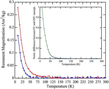
Figure 11. ZFC (in blue) and FC (in red) isothermal remanent magnetization (IRM) curves obtained using a 2.5 T magnetic induction applied at 10 K after cooling in zero field (ZFC) or in 2.5 T (FC). Inset: temperature evolution of the difference between the FC and ZFC dc susceptibility curves of Figure 8.

Discussion

The two magnetic components present in lepidocrocite are expressed differently in the different types of measurements performed. The Mössbauer signal is predominantly due to the antiferromagnetic γ-FeOOH matrix, the isothermal magnetization at moderate field contains equivalent contributions from both components and the dc and ac susceptibility signals are predominantly due to the ferrimagnetic nano-inclusions. These circumstances can be quite misleading. Indeed, since both the Mössbauer spectra and the susceptibility curves resemble those of superparamagnetic particles, one could be tempted to attribute both signals to the same entity, i.e., a volume distributed ensemble of lepidocrocite nanoparticles. However, the blocking temperatures for both techniques would then be almost the same: for Mössbauer spectroscopy, the temperature for which half the spectrum is paramagnetic-like (46.5 K for our sample), and for the dc magnetic measurements, the temperature for which the ZFC curve has its maximum (50 K for our sample). But their characteristic times are very different: τ_χ ≈ 100 s for the magnetic measurements and τ_M ≈ 10⁻⁸ s (the hyperfine Larmor precession time) for ⁵⁷Fe Mössbauer spectroscopy. This leads to a ratio of blocking temperatures: T${}_b^M$/T${}_b^{\chi }$ = ln(τ_χ/τ₀)/ln(τ_M/τ₀), where τ₀ = 10⁻⁹–10⁻¹² s, equal to 3–4, and consequently the two techniques cannot show the same T_b-value. Assigning T${}_b^{\chi }$ = 50 K to the ferrimagnetic nano-inclusions, its T${}_b^M$ should then be ~150 K, which explains why the Mössbauer sub-spectrum attributed to the nano-inclusions is a fully split hyperfine pattern at 77 K, i.e., it is in the “frozen” regime below T${}_b^M$. The fact that the Néel temperature of bulk lepidocrocite and the blocking temperature of the nano-inclusions are close (even almost the same in our sample) may thus be a coincidence.

We can tentatively identify this ferrimagnetic phase as maghemite γ-Fe₂O₃, or a phase closely related to maghemite, possibly located close to the rough surfaces of lepidocrocite particles. The mean particle size of 3.4 nm is close to the lower values of maghemite crystallite size (3–7 nm) determined by Till et al. (2014) initially formed during heating at low temperature of lepidocrocite. The saturation magnetization we obtain (ca. 75 Am²/kg) is close to the expected value for maghemite (74.3 Am²/kg at 300 K; Dunlop and Özdemir, 1997). The anisotropy density of 3.2 × 10⁵ J/m³ estimated from the ZFC data alone is larger than the effective anisotropy in maghemite (ca. 1.5 × 10⁴ J/m³; Hendriksen et al., 1994), but of the same magnitude as that found in other γ-Fe₂O₃ nanoparticles (Martinez et al., 1998), attributed to surface effects. Using a rather simple model of the ac magnetic susceptibility, we estimate the bulk anisotropy around 3 × 10⁴ J/m³, closer to that of Hendriksen et al. (1994) and the low-temperature surface anisotropy around 5 × 10⁻⁵ J/m². Using these values for a measurement time of 100 s would lead to a peak at 50 K as observed in the ZFC dc susceptibility measurements. Our model based on the presence of sparse nano-sized ferrimagnetic regions with less structural water, analogous to those observed by Till et al. (2014) during moderate heating, explains both the existence of the exchange bias and the limited range of the frequency dependence in χ′. Nonetheless, the values reported here are only estimates, as inter-particles interactions were not taken into account. Indeed, because the ferrimagnetic nano-particles are not directly observable (with only around 20 nanodots per 100 × 50 nm lepidocrocite particle), it is difficult to determine their spatial distribution and thus average inter-particles distances. Results are also likely dependent on the sample crystallinity. Due to the interplay of ferrimagnetic nanoparticles concentration, size distribution and interactions, the magnetic properties are expected to vary between samples. In the present study, the peak in χ′ is around 60 K and the ZFC/FC IRM curves merge at 100 K. In contrast, Hirt et al. (2002) report a peak in χ′ at 51.6 K, and ZFC/FC IRM curves merging at 250 K in their sample L89. In Till et al. (2014), the peaks in χ′ are located at 40 and 50 K, and the ZFC/FC IRM curves merge at 100 and 150 K for the slow and rapid syntheses, respectively. During the course of this study, we also examined by Mössbauer the lepidocrocite samples of Till et al. (2014). In the rapid synthesis sample, the ferrimagnetic particle mass fraction was estimated at 2% with a saturated M₀-value of 0.90 Am²/kg. In the slow synthesis sample, the ferrimagnetic particle contribution was not detectable in the Mossbauer spectra, but the saturated M₀-value was only 0.28 Am²/kg, much smaller than in the other samples. Therefore, the relative weight of the ferrimagnetic Mössbauer sub-spectrum does vary among samples, in good correlation with the M₀-value.

Author Contributions

YG lead the study, participated to magnetic measurements and numerical modeling. PB performed Mössbauer measurements, participated to magnetic measurements and numerical modeling. JT and GO participated to sample synthesis and characterization. FL participated in magnetic characterization. NM provided expertise in TEM.

Conflict of Interest Statement

The authors declare that the research was conducted in the absence of any commercial or financial relationships that could be construed as a potential conflict of interest.

Acknowledgments

This work was funded by project 2010-BLAN-604-01 from the French Agence Nationale de la Recherche (ANR). This is IPGP contribution number 3724.

References

Coey, J. M. D., Barry, A., Broto, J.-M., Rakoto, H., Brennan, S., Mussel, W. N., et al. (1995). Spin-flop in geothite. J. Phys. Condens. Matter 7, 759–768. doi: 10.1088/0953-8984/7/4/006

CrossRef Full Text | Google Scholar

Cornell, R. M., and Schwertmann, U. (2003). The Iron Oxides: Structure, Properties, Reactions, Occurrences and Uses. Weinheim: Wiley-VCH Verlag GmbH & Co.

Google Scholar

Cisowski, S. (1981). Interacting vs. non-interacting single domain behavior in natural and synthetic samples. Phys. Earth Planet. Int. 26, 56–62. doi: 10.1016/0031-9201(81)90097-2

CrossRef Full Text | Google Scholar

Cudennec, Y., and Lecerf, A. (2005). Topotactic transformations of goethite and lepidocrocite into hematite and maghemite. Solid State Sci. 7, 520–529. doi: 10.1016/j.solidstatesciences.2005.02.002

CrossRef Full Text | Google Scholar

De Grave, E., Persoons, R. M., Chambaere, D. G., Vandenberghe, R. E., and Bowen, L. H. (1986). An ⁵⁷Fe Mössbauer effect study of poorly crystalline γ-FeOOH. Phys. Chem. Miner. 13, 61–67. doi: 10.1007/BF00307313

CrossRef Full Text | Google Scholar

Dormann, J. L., Fiorani, D., and Tronc, E. (1997). “Magnetic relaxation in fine-particle systems,” in Advances in Chemical Physics, eds I. Prigogine and S. A. Rice (Hoboken, NJ: John Wiley and Sons, Inc.), 283–494.

Dunlop, D. J., and Özdemir, Ö. (1997). Rock Magnetism: Fundamentals and Frontiers. Cambridge, NY: Cambridge University Press.

Google Scholar

Eggleton, R. A., Schulze, D. G., and Stucki, J. W. (1988). “Introduction to crystal structures of iron-containing minerals,” in Iron in Soils and Clay Minerals, eds J. W. Stucki, B. A. Goodman, and U. Schwertmann (Dordrecht, Holland), 141–162.

Ewing, F. J. (1935). The crystal structure of lepidocrocite. J. Chem. Phys. 3, 420–424. doi: 10.1063/1.1749692

CrossRef Full Text | Google Scholar

Fitzpatrick, R. W., Taylor, R., Schwertmann, U., and Childs, C. (1985). Occurrence and properties of lepidocrocite in some soils of New Zealand, South Africa and Australia. Soil Res. 23, 543–567. doi: 10.1071/SR9850543

CrossRef Full Text | Google Scholar

Gilles, C., Bonville, P., Wong, K. K. W., and Mann, S. (2000). Non-Langevin behaviour of the uncompensated magnetisation in nanoparticles of artificial ferritin. Eur. Phys. J. B 17, 417–427. doi: 10.1007/s100510070121

CrossRef Full Text | Google Scholar

Gittleman, J. I., Abeles, B., and Bozowski, S. (1974). Superparamagnetism and relaxation effects in granular Ni-SiO₂ and Ni-Al₂O₃ films. Phys. Rev. B 9, 3891–3897. doi: 10.1103/PhysRevB.9.3891

CrossRef Full Text | Google Scholar

Greenwood, N. N., and Gibb, T. C. (1971). Mössbauer Spectroscopy. London: Chapman & Hall.

Gehring, A., and Hofmeister, A. (1994). The transformation of lepidocrocite during heating: a magnetic and spectroscopic study. Clays Clay Miner. 42, 409–415. doi: 10.1346/CCMN.1994.0420405

CrossRef Full Text | Google Scholar

Gendler, T., Shcherbakov, V., Dekkers, M., Gapeev, A., Gribov, S., and McClelland, E. (2005). The lepidocrocite–maghemite–haematite reaction chain I. acquisition of chemical remanent magnetization by maghemite, its magnetic properties and thermal stability. Geophys. J. Int. 160, 815–832. doi: 10.1111/j.1365-246X.2005.02550.x

CrossRef Full Text | Google Scholar

Hendriksen, P. V., Bodker, F., Linderoth, S., Wells, S., and Morup, S. (1994). Ultrafine maghemite particles I. studies of induced magnetic texture. J. Phys. Condens. Matter 6, 3081–3090. doi: 10.1088/0953-8984/6/16/013

CrossRef Full Text | Google Scholar

Hirt, A. M., Lanci, L., Dobson, J., Weidler, P., and Gehring, A. U. (2002). Low-temperature magnetic properties of lepidocrocite. J. Geophys. Res. 107, EPM 5-1. doi: 10.1029/2001JB000242

CrossRef Full Text | Google Scholar

Iglesias, O., Labarta, A., and Battle, X. (2008). Exchange bias phenomenology and models of core/shell nanoparticles. J. Nanosci. Nanotechnol. 8, 2761–2780. doi: 10.1166/jnn.2008.015

PubMed Abstract | CrossRef Full Text | Google Scholar

Johnson, C. E. (1969). Antiferromagnetism of γ-FeOOH: a Mössbauer effect study. J. Phys. C Solid State 2, 1996–2002. doi: 10.1088/0022-3719/2/11/314

CrossRef Full Text

Lee, G. H., Kim, S. H., Choi, B. J., Huh, S. H., Chang, Y., Kim, B., et al. (2004). Magnetic properties of needle-like α-FeOOH and γ-FeOOH nanoparticles. J. Korean Phys. Soc. 45, 1019–1024. doi: 10.3938/jkps.45.1019

CrossRef Full Text | Google Scholar

Liu, Q., Roberts, A. P., Larrasoana, J. C., Banerjee, S. K., Guyodo, Y., Tauxe, L., et al. (2012). Environmental magnetism: principles and applications. Rev. Geophys. 50, RG4002. doi: 10.1029/2012RG000393

CrossRef Full Text | Google Scholar

Martinez, B., Roig, A., Molins, E., Gonzalez-Carreno, T., and Serna, C. J. (1998). Magnetic characterisation of γ-Fe₂O₃ nanoparticles fabricated by aerosol pyrolysis. J. Appl. Phys. 83, 3256–3262. doi: 10.1063/1.367093

CrossRef Full Text | Google Scholar

Mermin, N. D., and Wagner, H. (1966). Absence of ferromagnetism or antiferromagnetism in one- or two-dimensensional isotropic Heisenberg models. Phys. Rev. Lett. 17, 1133–1136. doi: 10.1103/PhysRevLett.17.1133

PubMed Abstract | CrossRef Full Text | Google Scholar

Moskowitz, B. M., Frankel, R. B., Walton, S. A., Dickson, D. P. E., Wong, K. K. W., Douglas, T., et al. (1997). Determination of the preexponential frequency factor for superparamagnetic maghemite particles in magnetoferritin. J. Geophys. Res. 102, 22671–22680. doi: 10.1029/97JB01698

CrossRef Full Text | Google Scholar

Murad, E., and Cashion, J. (2004). Mössbauer Spectroscopy of Environmental Materials and their Industrial Utilisation. New York, NY: Springer.

Néel, L. (1949). Théorie du traînage magnétique des ferromagnétiques en grains fins avec application aux terres cuites. Annal. Géophys. 5, 99–136.

Ona-Nguema, G., Abdelmoula, M., Jorand, F., Benali, O., Géhin, A., Block, J., et al. (2002). Iron (II, III) hydroxycarbonate green rust formation and stabilization from lepidocrocite bioreduction. Environ. Sci. Technol. 36, 16–20. doi: 10.1021/es0020456

PubMed Abstract | CrossRef Full Text | Google Scholar

Özdemir, Ö., and Dunlop, D. J. (1996). Thermoremanence and Néel temperature of goethite. Geophys. Res. Lett. 23, 921–924. doi: 10.1029/96GL00904

CrossRef Full Text | Google Scholar

Till, J. L., Guyodo, Y., Lagroix, F., Ona-Nguema, G., and Brest, J. (2014). Magnetic comparison of abiogenic and biogenic alteration products of lepidocrocite. Earth Planet. Sci. Lett. 395, 149–158. doi: 10.1016/j.epsl.2014.03.051

CrossRef Full Text | Google Scholar

Tronc, E., Prené, P., Jolivet, J.-P., d'Orazio, F., Lucari, F., Fiorani, D., et al. (1995). Magnetic behaviour of γ-Fe₂O₃ nanoparticles by Mössbauer spectroscopy and magnetic measurements. Hyperfine Interact. 95, 129–148.

Google Scholar