A New Method for Comparing and Matching Snow Profiles, Application for Profiles Measured by Penetrometers

1. Introduction

Avalanches are a major danger in mountainous areas that threatens human life and infrastructure. Snow cover stratigraphy, i.e., the vertical arrangement of snow layers with different physical properties, is a key factor of slab avalanche formation (Schweizer et al., 2003). The presence of a weak layer below a relatively cohesive slab is, in particular, a prerequisite for the release of dry snow slab avalanches. The standard representation of this snowpack stratigraphy is one dimensional (1D) and consists of the superposition of numerous homogeneous slope-parallel layers (Fierz et al., 2009). This idealization is used for numerical modeling of snowpack evolution (Brun et al., 1992; Vionnet et al., 2012) and for educational purposes (e.g., at the snow study center). It is motivated by the fact that inter-layer vertical variability (lithological variability) generally dominates horizontal variability (spatial variability) on the snow pit scale (Birkeland K. W. et al., 2004).

It is often observed, however, that vertical snow profiles measured several meters from each other are different, making it difficult to identify a 1D depth profile (of snow properties) representative of the test site. Such discrepancy between profiles can be explained by snowpack spatial variability or by depth positioning errors. Indeed, errors in the depth measured can create an apparent spatial variability. The true spatial variability on a decameter scale is mainly due to the wind in cold winter months (Kronholm et al., 2004). This factor leads to a continuous depth-variation of the snow layers but preserves the main features of the profiles, when these are measured within tens of meters distance in smooth terrain (Harper and Bradford, 2003; Kronholm et al., 2004; Tape et al., 2010). Spatial variation of snow layer depth may affect snow internal processes such as pressure sintering, and may therefore yield spatial variability in intensive properties such as density or hardness (Schweizer et al., 2008). No clear trend in the evolution of spatial variability has however been observed so far with time (Harper and Bradford, 2003; Logan et al., 2007; Schweizer et al., 2008).

Such true and apparent spatial variability causes stratigraphic mismatches, even if continuous layers are observed to be present in the snowpack (Sturm and Benson, 2004). Points at the same depth are not necessarily at the same position in the stratigraphy; they do not have the same age nor share the same history. The matching between layers identified by an observer at nearby locations can be performed manually for a small number of profiles and layers (e.g., Sturm and Benson, 2004). However, with the development of portable high-resolution snowpack profilers such as digital penetrometers (e.g., Schneebeli and Johnson, 1998), or specific surface area profilers (e.g., Arnaud et al., 2011), it is now possible to perform numerous tests on the same site within a short time, and the resulting wealth of data provides inputs for estimating spatial variability that is no longer possible to process manually across the measurement points. The data thus requires an automatic matching method that synthesizes multiple profiles into the classical 1D representation of the snowpack stratigraphy. This paper presents a new matching method for this purpose.

Various studies have proposed methods for tracking layers in space to investigate snow spatial variability on the slope scale or compare snow profiles with each other. These are reviewed here. Harper and Bradford (2003), Sturm and Benson (2004), Birkeland K. W. et al. (2004), and Kronholm et al. (2004) tracked layers manually from point measurements in order to assess snow spatial variability. Layer tracking was performed manually because no adequate automatic algorithms existed for layer identification (Birkeland K. W. et al., 2004; Kronholm et al., 2004). Tape et al. (2010) tracked layers manually through the use of close-up infrared photography of a snow trench. Vertical cross-section plots of the snow hardness profiles also give an overview of the spatial variability and facilitate this manual tracking (Proksch et al., 2015), but these plots are limited to the representation of points distributed on a given transect and are inappropriate for 2D (in plan view) and uneven distribution of measurement points. Lutz and Marshall (2014), Floyer (2008), and Pilloix and Hagenmuller (2015) also used manual tracking to evaluate the accuracy of the depth sensor of the Avatech SP1 and SABRE penetrometers. Floyer and Jamieson (2008) proposed an automatic method based on a Wiener spiking deconvolution algorithm in order to track weak layers across a grid of hardness profiles. To our knowledge, this method is the only semi-automatic tracking method used in the snow and avalanche community. This method successfully tracks distinct features such as crusts and weak layers not in proximity to crusts, but failed to identify less distinct features such as gradual hardness transitions (Floyer and Jamieson, 2008). Herwijnen et al. (2009) used a similar method for tracking failure layers identified by a compression test. This method is however limited to the tracking of one particular feature such as a weak layer and does not exploit the fact that profiles can also share similar stratigraphic sequences, e.g., alternating crust and soft layers. In order to compare simulated snow profiles to observations, Lehning et al. (2001) implemented a mapping method adjustable for deviating total snow depth and layer segmentation. A method for co-registering multiple hardness profiles using multiple trackable stratigraphic sequences is currently lacking. Up until now, this was done manually, or by a semi-automatic method limited to the tracking of one specific layer.

In this article, we introduce an approach to match and track multiple layers in snow profiles. We apply this method to hardness profiles collected by digital penetrometers (snow micropenetrometer, Avatech SP1) and the ramsonde. The objectives are (1) to synthesize the information collected in several depth profiles into one representative profile and disentangle information about hardness and depth variabilities and (2) to compare quantitative hardness profiles measured at the same sites by different penetrometers. Firstly, the penetrometers, the test sites and our matching algorithm are presented. The method is then applied to two measurement sets in order to illustrate its ability to track layers whose origin is inferred to be linked to wind events. Its ability to build a representative profile despited limited accuracy of the depth sensor of the penetrometer is also presented. Finally, the outcomes and limitations of this method are discussed.

2. Materials and Methods

2.1. Penetrometers

Snow hardness, defined as the resistance against penetration of an object in snow (Fierz et al., 2009), has long been recognized as a good indicator of snow mechanical properties (Bader and Niggli, 1939; Marshall and Johnson, 2009) and thus as an indicator of avalanche-prone stratigraphies. Penetration tests are relatively easy to set up in the field, so snow hardness remains a measure of choice for snowpack stratigraphic observations, both within the framework of operational avalanche forecasting (e.g., as taught to Meteo-France forecasters at the snow study center) and recent research about snow and avalanches (e.g., Proksch et al., 2015; Reuter et al., 2015).

Snow hardness can be qualified by hand and measured by penetrometers. The original penetrometer is the ramsonde adapted from soil mechanics to snow studies by Haefeli in the 1930s (Bader and Niggli, 1939). Many developments have since been made to improve the instrument's sensitivity and ease of use (see exhaustive review of Floyer, 2008). The range of penetrometers available currently are not used systematically in the field, and the ramsonde remains the reference instrument for operational avalanche forecasting purposes (Fierz et al., 2009). However, among the more successful developments are the snow micropenetrometer (SMP), a highly sensitive digital penetrometer composed of a small tip, the penetration of which is controlled by a motor (Schneebeli and Johnson, 1998), and the SABRE, a portable manually-driven penetrometer using an accelerometer to measure penetration depth (Mackenzie et al., 2002). Also, a commercial version of the latter kind of digital penetrometer, the SP1, has recently been developed by the company Avatech. In this paper, we examine profiles measured by the SMP, the SP1 and the ramsonde.

2.1.1. Snow Micropenetrometer (SMP)

The snow micropenetrometer (SMP) measures high-resolution profiles at fast acquisition times. Its high resolution also enables the interpretation of penetration force fluctuations for microstructural parameters (e.g., Satyawali et al., 2009; Proksch et al., 2015). However, its high cost (around 40,000 dollars in 2011) and weight (around 7 kg), and its relative fragility compared to other penetrometers restrain its usage to research purposes as opposed to operational avalanche forecasting.

For this study, the 4th version (SMP4) of the device developed by Schneebeli and Johnson (1998) was used. The SMP consists of a measuring conic tip with a 60° apex angle and a maximum diameter of 5 mm, which is driven into the snowpack by a motor with a constant speed of 20 mm s⁻¹ (Figure 1A). 250 force measurements are recorded per millimeter at this speed. The profiles are measured vertically, with the motor held fixed above the snow surface on a table composed of ski poles. Due to slight movements of the motor when the tip hit hard layers, the depth accuracy is estimated to be roughly 1 cm. The maximum measured depth, 1.6 m, is restricted by the instrument's length. The force sensor measures in the range [0,40] N, with a resolution of 0.01 N. We report to the SMP hardness or penetration strength as the measured resisting force divided by the maximal horizontal cross-section area (19.6 mm²) of the SMP measuring tip.

FIGURE 1

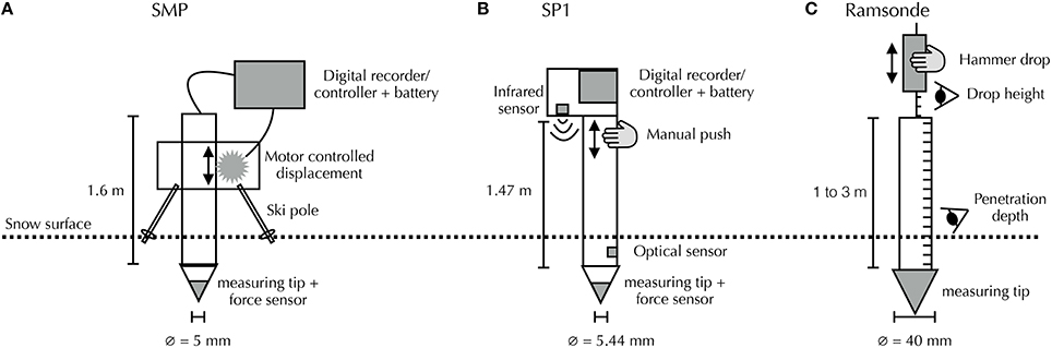
Figure 1. Main features of the three penetrometers used in this study: (A) SMP, (B) SP1 and (C) ramsonde. The diagrams are not to scale.

2.1.2. Avatech Snow Probe 1 (SP1)

In September 2014, Avatech (www.avatech.com) commercialized the Snow Probe 1 (SP1), a light weight “rapid-push” snow penetrometer. This instrument is easy to use and transport in the field. It is intended for use by snow professionals including ski patrollers, mountain guides and avalanche forecasters (Lutz and Marshall, 2014).

The SP1 consists of a measuring conic tip with a 60° apex angle and a maximum diameter of 5.44 mm, which is pushed manually into the snowpack (Figure 1B). The SP1 has to be pushed down vertically by 1.5 m in a time between 0.5 s and 1.5 s, leading to a penetration speed in the order of 1 m s⁻¹. A force measurement is recorded every millimeter. The profiles were measured vertically to a maximum depth of 1.47 m. Depth is calculated by combining the signals of an infrared sensor, an optical sensor and the tip force sensor. The infrared sensor, located at the top of the probe facing the snow surface uses reflection intensity and angle to compute distance to the surface. The optical sensor, located at the bottom of the probe, and the force sensor detect whether the tip has entered the snowpack and their outputs are used to scale the measured depth. According to the SP1 manual (Avatech, 2014), the potential errors in depth is 15 cm for depths between 0 and 40 cm, 10 cm for depths between 40 and 80 cm, and 4 cm for depths between 80 and 147 cm. The force sensor measures forces between 0 and 23 N with an accuracy of 0.7 N. We report to the SP1 hardness as the measured resisting force divided by the maximal horizontal cross-section area (23.2 mm²) of the SP1 measuring tip.

2.1.3. Ramsonde

Because of its robustness and simplicity, the ramsonde is the standard instrument for measuring hardness. The ram hardness is still used by avalanche forecasters and remains the main mechanical variable simulated by snowpack models (e.g., Durand et al., 1999).

The ramsonde consists of a 1 m tube ending in a conic tip with a 60° apex angle and a maximum diameter of 40 mm (Figure 1C). Extension tubes can be added to probe deeper snowpacks. The ramsonde is driven into the snowpack by dropping a hammer of weight P on top of the probe. For a certain number (n) of drops from a given drop height (h), the penetration depth increase (e) is manually recorded. The penetration resisting force (R) is calculated as R = nhP∕e+P+Q, with Q being the total weight of the tubes. Unlike the SMP and SP1, which are displacement-controlled, the ramsonde is force-driven, so its depth resolution depends on the snow hardness—it is at best 1 cm for hard snow (Pielmeier and Schneebeli, 2003). The penetration velocity is not constant. The hardness resolution depends on the drop height chosen by the observer and is limited by the weight of the tubes and of the hammer. We refer to the ramsonde hardness (“ram hardness”) as the measured resisting force R divided by the maximal horizontal cross-section area (1260 mm²) of the ramsonde tip.

2.2. Study Area and Snow Measurements

2.2.1. Col du Lautaret

Snow hardness profiles were collected in the French Alps, next to the Lautaret Pass at 2076 m above sea level (a.s.l.) on January 21, 2015. The sky was overcast with moderate wind. The site is located below a small ridge oriented perpendicularly to the main wind direction (SE) on a 10° slope facing NW. As experienced during the measurements, the snow layer thicknesses in the zone were highly variable because of extensive snow deposition and transport by wind. This site was selected because of the resulting snowpack heterogeneity. Snow profiles are here described according to the classification scheme of Fierz et al. (2009) (Figure 2A), and five SMP measurements and three ramsonde measurements were measured on a 50 cm long line along the wind trajectory (Figure 3A).

FIGURE 2

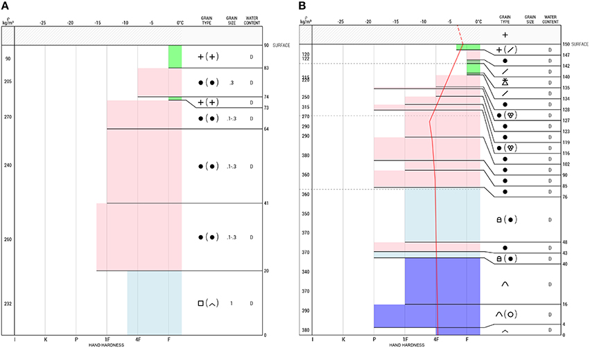
Figure 2. Stratigraphy of the snowpack observed at (A) Col du Lautaret and (B) Glacier de la Girose. Visualization adapted from avanet.avatech.com. Colors and symbols of the international classification are used (Fierz et al., 2009).

FIGURE 3

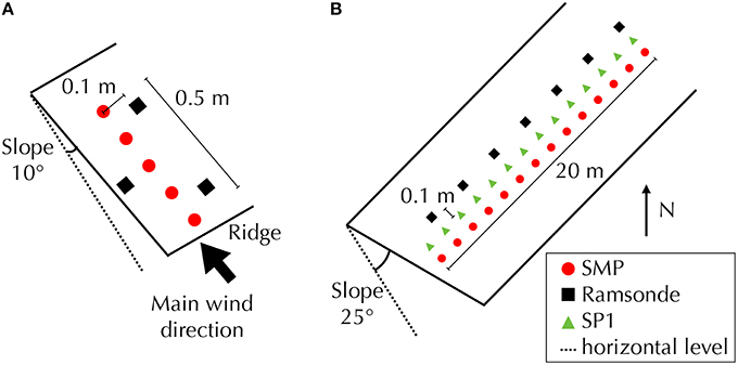
Figure 3. Measurement configuration at (A) Col du Lautaret and (B) Glacier de la Girose. The scheme is not to scale.

2.2.2. Glacier de la Girose

The second test site is located in the French Alps on the Girose Glacier at 3277 m a.s.l. Measurements were conducted on 23 March 2015 on a large and homogeneous slope with an angle of 25° that is NW oriented. The weather was sunny without wind (SP1 infrared sensor oriented in the shadow). The site is situated on smooth terrain far from ridges, and selected for the homogeneity of its snowpack and its high elevation, which ensured dry snow at the time of measurement. The measured stratigraphy was classified according to Fierz et al. (2009) (Figure 2B), and 14 SP1, 14 SMP and 7 ramsonde hardness profiles were recorded on a 20 m long line perpendicular to the slope (Figure 3B). The SP1 and SMP profiles were co-located and measured within no more than 10 cm from each other. One every two SP1/SMP profiles was complemented by a ramsonde profile, measured within a maximum distance of 10 cm (Figure 3B).

2.3. Matching Algorithm

To track layers in the snowpack, we conduct 1D signal registrations on the hardness profiles provided by the penetrometers. Registration consists of retrieving the transformation that best matches points of similar characteristics. Registration requires three main components: a transformation function, a similarity metric, and an optimizer that finds the best transformation given the similarity metric. In this section, each of these components is explained.

1. Snow profile transformation. A hardness profile represents the penetration strength σ₀ as a function of depth h₀. The depth points are not unique but depend on the penetrometer and the instrument set-up. To regularize all profiles for equal treatment, each hardness profile is first re-sampled onto a certain depth grid h (Figures 4A,B). A regular depth grid with constant vertical step Δh is used here. The re-sampled hardness profile is denoted (σ, h). The re-sampling is performed through the convolution with a Gaussian kernel of standard deviation Δh and linear interpolation. The vertical step Δh defines the profile resolution, i.e., the thinnest snowpack feature preservable by the record after re-sampling. As explained in the Introduction, much of the spatial variability of the snowpack is expected to come from layer depth deviations between profiles. The transformation procedure modifies the depth h by stretching or thinning different layers by different amounts. To preserve the ordering of layers, the transformation is applied to layer thickness and not to layer depth. To this end, the snowpack is first decomposed onto a specified 1D vertical grid of layers of uniform thickness Δl (Figure 4B). These layers do not necessarily have physical meaning; they merely define the support of the transformation. The chosen transformation T consists of thinning or stretching the thickness Δl of layer j by a certain factor α_j, i.e., the new thickness of layer j is α_j × Δl (Figures 4B,C). The new depth points h_T of the hardness measurements σ are then easily derived from the layer thicknesses. The thinning or stretching factor is constant for each layer, and even though the layer is not necessarily constant in terms of hardness. The layer grid step Δl is greater than the vertical depth step Δh, so as to preserve the high resolution of the hardness profile whilst keeping a relatively low number of degrees of freedom {α_j} for the transformation. The transformed depth points h_T do not necessarily lie on to the regular grid points h (Figure 4C). The transformed profile (σ, h_T) is thus linearly interpolated on the regular depth grid to obtain the final profile (σ_T, h) (Figure 4D).

2. Similarity metric. This metric quantifies how similar different profiles are. The hardness of an initial or transformed profile, here simply denoted σ for convenience in notations, is used to define this metric. We distinguish two metrics: a distance D between one profile and a reference profile, and an intra-set variability V of a set of multiple profiles.

a. Distance D between two profiles. The distance D between two profiles (σ, h) and (σ_ref, h) re-sampled on the same depth grid h is defined as the mean square difference of the hardness in a log-scale, i.e.:

$\begin{array}{rc}D=\frac{1}{h_{\text{tot}}}{\displaystyle {\int }_0^{h_{\text{tot}}}{(\log {\sigma }_{ref}(x)-\log \sigma (x))}^{2}d}x& (1)\end{array}$

with h_tot being the total snow depth. The log-scale permits one to assign as much importance to the hard layers as to the soft (including weak) layers.

b. Intra-set variability V. The intra-set variability V quantifies how different several profiles are from each other without appointing one of them as the reference. It is defined as the standard deviation of the hardness logarithm for a given height between different profiles, averaged on the height., i.e.:

$\begin{array}{rc}V=\frac{1}{h_{\text{tot}}}{\displaystyle {\int }_0^{h_{\text{tot}}}{\left(\frac{1}{n_p}{\displaystyle \sum _{p\in P}{(\log {\sigma }_p(x)-\overline{\log \sigma (x)})}^2}\right)}^{0.5}dx}& (2)\end{array}$

with n_p being the total number of profiles# P the profile set and $\overline{X}$ the mean value of X in the profile set for a given height. The considered profiles must be re-sampled on the same depth grid to compute V (see above).

3. Optimization. The optimum values of α_j are those which minimize the distance D between a transformed profile and a reference profile, or minimize the intra-set variability V of several transformed profiles. We, hereafter, called “auto-matching” the procedure of matching several profiles together. The value of the factor α_j is constrained. Firstly, α_j is bounded in a certain range [1−ϵ, 1+ϵ] with ϵ a constant positive parameter, to avoid non-physical transformations, e.g., α_j < 0 or α_j ≫ 1. There are other constraints on α_j as detailed in the following. The accuracy of the SP1 local depth sensor is expected to be poor but it can recover the total snow depth with a good accuracy (see Section 2.1.2). In the case of a homogeneous snowpack, the matching of one SP1 profile to a reference profile can use this information, expressed in terms of constraints on α_j as $1-{E}\le \sum _j{\alpha }_j\le 1+{E}$, with ${E}$ a constant positive parameter. For instance, a value ${E}$ = 0.2 means that the total height of the transformed profile cannot be dilated or thinned by more than 20% of the initial total height. When the intra-set variability V is minimized via this technique, the latter constraint on $\sum _j{\alpha }_j$ is not taken into account but the mean of all profile transformations for the same layer is set to the identity, which means that for each layer $\sum _{\text{profile}}\alpha =n_p$ with n_p representing the number of profiles. This constrained optimization problem is considered by the method SLSQP (Sequential Least Squares Programming, implemented in python package scipy.optimize) (Kraft, 1988). The initial seed for α in the optimizer is 1; in other words the transformation is initialized with the identity transformation.

FIGURE 4

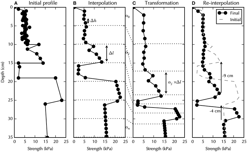
Figure 4. Example of a snow profile transformation. The initial profile (A) is re-sampled on a regular depth grid with a depth step Δh (B). Then, the different layers of thickness Δl are stretched or thinned by a certain factor α_j (C). Finally, the transformed profile is re-interpolated on to the depth grid (D). Two examples of depth changes (−9 and −4 cm) between initial and transformed profiles are shown.

The developed algorithm enables the transformation of a profile to match a given reference profile according to D, or to transform multiple profiles so that their intra-set variability V is minimal. The algorithm depends on different parameters: Δh the depth grid resolution, Δl the thickness of the layer used to transform a profile, ϵ which defines the bounds of the stretching/thinning factor, and possibly ${E}$ which defines a bound on the total thickness transformation. The values used in this study are described in Table 1. The choice of the parameters Δh and Δl is related to the vertical resolution of the penetrometer and the size of the hardness features of the tested snowpack. A sensitivity analysis showed no impact of Δh in the range [0.05, 0.5] cm and of Δl in the range [2, 6] cm on the matched profile sets of the SP1 and SMP. The choice of the parameter ϵ poses a constraint on the maximum variability in layer thickness to be accounted for. No significant influence of ϵ in the range [50, 90]% on the matching results was observed. The value of the parameter ${E}$ was set according to the expected accuracy of the SP1 to recover the total snow depth.

TABLE 1

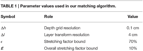
Table 1. Parameter values used in our matching algorithm.

3. Results

3.1. Spatial Variability

In this section, the matching algorithm is applied to the SMP measurements of the two test sites. The main idea is to synthesize the measured data into a single representative profile including information about the intra-set variability of layer thickness and hardness.

Figure 5A shows the initial SMP measurements on the Lautaret site. For the first 40 cm, the hardness profiles are clearly correlated. Below 40 cm, it is very difficult to visually identify similar features between the profiles. The median hardness profile reveals a potential slab structure with a weak layer at a depth of 10 cm depth and no other particular structure below. Figure 5B shows the transformed profiles that minimize the intra-set variability. All data combine to form single trend with less variability at a given depth. The mean coefficient of variation per layer decreases from 36 to 18% with the matching. The median of these profiles is representative of the test site. The algorithm reveals a clear slab structure with the continuous presence of a weak layer at a depth of 65 cm depth on average. The penetration strength of this weak layer is heterogeneous with a median value of 20 kPa, a minimum value of 5 kPa and a maximum value of 30 kPa. In every profile, there is a sharp transition between a relatively hard layer located between depths of 50 and 65 cm and this weak layer. The transition is emphasized by the algorithm and is invisible if the initial profiles are simply plotted next to each other. This observation agrees with the presence of faceted crystals at this depth (Figure 2A). Figure 5C indicates the depth transformations necessary to convert the matched profiles (Figure 5B) back into the initial profiles (Figure 5A). As expected, the amplitude of the depth transformations increases with depth. The gradient of the difference in depth reflects the intra-set variability in layer thickness. It appears that the layer located between 30 and 45 cm depth in the transformed profile is mostly responsible for the observed snowpack variability with a thickness varying in the range [8, 22] cm. Through this approach, the intra-set profile variability is decomposed into hardness variability (Figure 5B) and layer depth variability (Figure 5C).

FIGURE 5

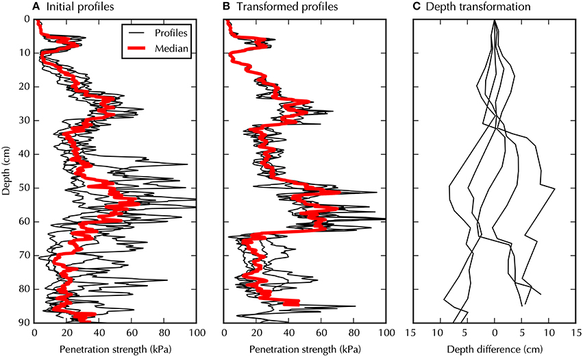
Figure 5. Auto-matching of the SMP profiles measured at Col du Lautaret. (A) The initial profiles re-sampled on to the depth grid. (B) Profiles transformed so that the their intra-set variability is minimized. Each initial profile is transformed by its own set of stretching factors. The median profile (red curve) is chosen as representative of the set. (C) Depth changes between transformed profiles (B) and initial profiles (A). Adding these changes to the matched profiles depth (B) recovers the initial profiles (A). These depth transformations are derived from the values of α determined by the optimizer.

The same approach was applied to the SMP data of the Glacier de la Girose (Figure 6). The snowpack is more homogeneous at this site and the main stratigraphic features can be followed without applying the matching algorithm (Figure 6A). The matched profiles, however, collapse on a single profile with surprisingly little intra-set variability. This finding emphasizes the horizontal homogeneity of the snowpack (Figure 6B). Even at a distance of tens of meters, features at centimeter scale can be followed with depth variations of a few centimeters (Figure 6C). The mean coefficient of variation per layer decreases from 40 to 20% with the matching. Note that these coefficients of variation are calculated from profiles measured on a 20 m line and thus appear slightly larger than those calculated on the 50 cm line of Col du Lautaret, even if the snowpack of Glacier de la Girose is more homogeneous.

FIGURE 6

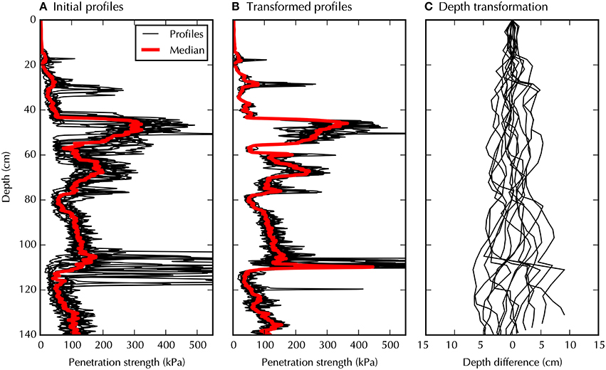
Figure 6. Auto-matching of the SMP profiles measured at Glacier de la Girose. The same approach is used as in Figure 5 but applied to a more homogeneous snowpack.

3.2. Instrumental Depth Variability

In this section, the matching algorithm is used to assess and reduce depth variability caused by depth measurement errors.

3.2.1. Comparison between SP1 and SMP Profiles

Each SP1 profile was obtained within a 10 cm distance of a SMP profile. The depth obtained with the SMP can be considered as a reference since its depth accuracy is estimated to be less than 1 cm. We therefore can evaluate the quality of the SP1 profile (its accuracy in depth and hardness) by matching it to the SMP profile.

Figure 7A shows an example of two co-located SMP and SP1 profiles measured at Glacier de la Girose. In this example, the main difference between the SP1 and SMP profiles originates from the SP1 depth sensor and not from its force sensor. The SP1 profile needs to be translated locally by up to 17 cm to match the SMP profile. The SP1 hardness agrees well with that of the SMP after matching, which reduces the root mean square difference from 123 kPa to 24 kPa.

FIGURE 7

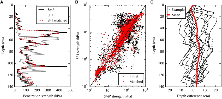
Figure 7. Matching of the SP1 profiles to the SMP profiles measured at Glacier de la Girose. Fourteen co-located SP1/SMP profiles were processed. (A) One example of two matched profiles. (B) SP1 hardness as a function of the SMP hardness with and without matching. (C) Depth changes used to match the profiles. The depth transformation used for the example shown in (A) is plotted with a dotted gray line. The mean value (red line) corresponds to the depth transformation for each layer averaged on the profile set.

This matching was reproduced on the 14 co-located SP1 and SMP profiles measured at the Glacier de la Girose (Figures 7B,C). It confirms the good agreement in the hardness measured with the two instruments. The root mean square difference decreases from 120 kPa to 49 kPa when the profiles are matched (Figure 7B). The matching indicates that SP1 depths have to be adjusted locally by depth changes in the range of [−17, 20] cm; the changes have an overall standard deviation of 7.7 cm and a mean absolute standard deviation per layer of 4.1 cm (Figure 7C). Given the accuracy of the SMP depth sensor and the homogeneity of the snowpack on a scale of 10 cm on this site (see Figure 6), the changes in depth derived from the matching reflect mainly depth measurement errors in the SP1.

3.2.2. Method to Reduce SP1 Depth Discrepancy

Based on the Glacier de la Girose measurements, the SP1 depth errors were evaluated in the range of [−17, 20] cm and were shown to be larger close to the snow surface (Figure 7C). No large bias on the depth errors was observed however (Figure 7C and mean absolute standard deviation per layer of 4.1 cm). It therefore appears possible to reduce this depth discrepancy by matching multiple SP1 profiles together, without using an independent reference profile (e.g., SMP). The principle is the same as that presented in Section 3.1 but, here, the depth transformation accounts for both spatial variability and instrumental depth errors and cannot distinguish between these two components.

The initial SP1 profiles are shown in Figure 8A. As expected, depth errors make it impossible to identify common features shared by these profiles, even if the snowpack is horizontally homogeneous at this site. Minimization of the intra-set variability successfully recovers the general structure of the snowpack (Figure 8B). The depth transformation used to auto-match the SP1 profiles are consistent with the transformation used to match the SP1 profiles to the SMP profiles (Figures 7C, 8C). However, the residual intra-set hardness variability found here exceeds the variability found from the matching previously performed on the SMP data at the same site (Figure 6B).

FIGURE 8

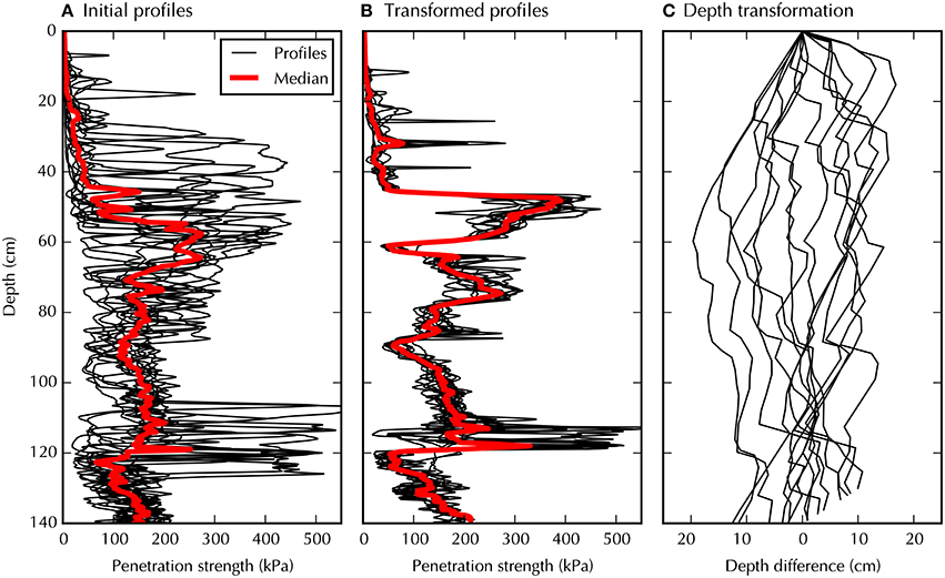
Figure 8. Auto-matching of the SP1 profiles measured at Glacier de la Girose. The same approach is used as in Figure 5 but applied to the SP1 measurements of the horizontally homogeneous snowpack at Glacier de la Girose. In this dataset, the depth variability originates mainly from the low reproducibility of the SP1 depth sensor.

In Figure 9A, the auto-matched SP1 profile is compared to the auto-matched SMP profile calculated in Section 3.1. The main hardness features detected by the SMP are recovered by the SP1. Differences in depth remain, however (Figure 9B). Indeed, to match these two profiles, the SP1 depths have to be adjusted locally by depth changes in the range of [−3, 10] cm; the changes have an overall standard deviation of 3.5 cm and and an absolute mean of 4.1 cm. The maximum depth deviation appears at a depth of around 80 cm, not near the snow surface. The mean absolute depth difference (4.1 cm) is equal to the one computed with the matching to the reference SMP profiles, and this result shows the robustness of the approach. The matched SP1 profile illustrates that the hardness measured with the SP1 is very similar to the hardness measured with the SMP. This observation indicates that at a depth resolution Δh = 0.1 cm, both instruments' hardnesses are comparable despite their differences in the strain rate and tip size.

FIGURE 9

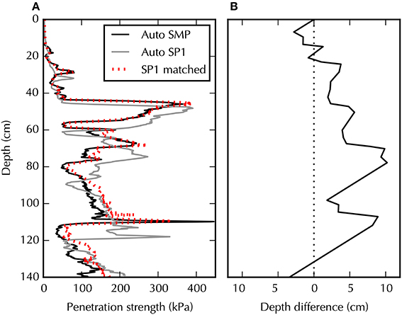
Figure 9. Comparison of the SP1 and SMP auto-matched profiles measured at Glacier de la Girose. (A) Matching of these two profiles. (B) Depth changes used to match these two profiles.

3.2.3. Ramsonde Profile: Variability Due to Operator Practices

The co-located ram and SMP profiles were also matched with the presented algorithm. However, this matching did not significantly improve the hardness-profile correspondence between these instruments. The effects of the loading conditions (tip size and deformation velocity) are important and mask small possible depth differences which could have been detected by the matching approach. Contrarily to the hardness measured with the SP1 which tip size and deformation velocity are of the same order of magnitude as the SMP, the absolute value of the ram hardness cannot be directly compared with the SMP penetration strength (Pielmeier and Schneebeli, 2003).

However, the ram profiles themselves can be matched to assess the impact of operator practices (hammer drop height and number of drops) on them. Figure 10 shows the auto-matched ram profiles measured at Glacier de la Girose. The depth transformations used to match the ram profiles have a similar range as that observed to match the SMP profiles. The remaining intra-set variability in hardness is partly due to the spatial variability of strength and also to operator practices. Indeed, some features shown to have negligible hardness variability by both the SMP and SP1 profiles, such as the soft layer located around a depth of 60 cm (see Figures 6B, 8B, 10B), appear in the matched ram profiles with significantly higher variability. This variability is explained by the fact that operator practices during a ramsonde measurement affect not only the position of layer boundaries (Figure 10C) but also the hardness sensitivity itself (Figure 10B). This effect is particularly notable on a soft layer located just below a hard layer (Figure 10B). In practice, the operator must anticipate the presence of this weak layer and decrease the drop height before entering this soft layer in order to capture its low penetration resistance.

FIGURE 10

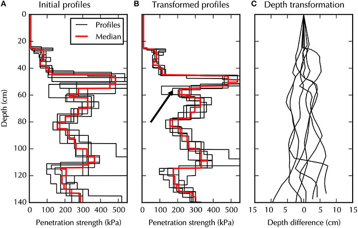
Figure 10. Auto-matching of the ram profiles measured at Glacier de la Girose. The same approach is used as in Figure 5 but applied to the ram profiles measured at Glacier de la Girose. The arrow on (B) identifies a soft layer, whose hardness variability is interpreted to be due to operator practice.

4. Discussion and Conclusion

The measured thickness of snow layers varies along slope due either to true spatial variability or to potential errors in vertical positioning. In consequence, points inside the snowpack, located at the same depth but different slope-parallel positions are not necessarily at the same position in the stratigraphy. The referencing in terms of depth thus creates an apparent spatial variability in the stratigraphy (Sturm and Benson, 2004). The matching algorithm developed in this study disentangles this variability by separating it into hardness and depth variabilities. On wind-exposed sites with significant variability in layer thicknesses with horizontal position, such as at Col du Lautaret, layers were successfully tracked over a 50 cm transect, even if the layer thicknesses varied by a factor of two. For the horizontally homogeneous snowpack on the Glacier de la Girose, layers at centimeter scale, with negligible hardness variability were tracked along a transect 20 m long. Our ability to track thin layers on a decameter scale using our matching algorithm confirms that, even if the snowpack appears to be highly variable, it is worth measuring detailed point features, which can provide information relevant at a larger scale.

A time-consuming but essential part of spatial variability analysis is the manual matching of the stratigraphic sequence (e.g., Kronholm et al., 2004). For this reason, previous studies have focused on a relatively few number of layers (e.g., 11 layers by Kronholm et al., 2004, 5–10 layers by Sturm and Benson, 2004). However, as noticed by Birkeland K. et al. (2004), if layers are merged together, then the spatial structure is less apparent than when the layers are analyzed separately. The presented algorithm makes this processing automatic with a vertical resolution adaptable to the resolution of the instrument.

The basic assumption underlying the presented algorithm is that depth deviations explain most of the observed variability. This assumption makes sense when the vertical profile of hardness or other intensive properties are not heavily affected by other external drivers such as solar radiation, vegetation, etc. More generally, the matching is performed using additional information about the physics of snowpack evolution. For instance, Lemieux-Dudon et al. (2010) developed an ice core age scale based on an inverse method combining glaciological modeling with absolute and stratigraphic markers. We used the simplistic assumption that the spatial variability is induced by snow redistribution and precipitation and that this variability does not induce changes in intensive properties such as hardness. One further step would be to incorporate physical processes into the profile transformation function. In particular, the depth transformation could be coupled to layer compaction laws depending on the overburden, as described by Vionnet et al. (2012).

In this study, the matching algorithm was applied to multiple measured hardness profiles, and the computed depth variability was attributed to wind and precipitation events and measurement errors. The algorithm could be further used to compare modeled and measured hardness profiles. Indeed, the calibration and testing of snow cover models is notoriously difficult due to snowpack heterogeneity and uncertainties in atmospherical forcings, especially the amount of precipitation. In contrast, Lehning et al. (2001) proposed a method for comparing modeled and measured profiles that accounts for the total depth deviation, but that assumes that the computed stretching factor applies equally to all layers. In our method, the transformation obtained from the matching of hardness profiles can account for layer thickness deviations due to single precipitation or wind events. The calculated transformation can be applied to profiles of other properties such as the specific surface area or the grain type, which provides a direct way for evaluating snow-cover models, overcoming the limited accuracy of atmospheric forcings.

New ensemble simulations of snowpack conditions produce numerous snow profiles which capture the uncertainty in meteorological forcings (Vernay et al., 2015). In the framework of operational avalanche forecasting, the proposed algorithm is also a practical method for combining of this wealth of data into synthetic information concerning the snowpack layering.

Our algorithm is generic and is applicable on any depth–penetration strength profile provided by a penetrometer. It is applied here to profiles measured by commonly-used penetrometers in typical field situations. The metrics D and V between profiles whose definition involves the mean square difference of logarithmic hardness can be adapted to incorporate vertical profiles of other snow properties. For instance, the vertical profiles of specific surface area, such as that measured by ASSSAP (Alpine Snowpack Specific Surface Area Profiler) (Arnaud et al., 2011) could be employed instead of hardness, or combined with hardness, when profiles are matched. Alternatively, the correlation length derived from the SMP hardness, which is an indicator of the specific surface area (Proksch et al., 2015), could be combined with the SMP hardness in the distance function.

The matching algorithm was used to evaluate quantitatively the SP1 in in-situ field measurements. The SP1 hardness is shown to agree with the SMP hardness, but the depth derived from the SP1 infrared sensor is inaccurate, with sizeable errors having a standard deviation of 7.8 cm and maximum deviation of 20 cm at the considered site. Combining several SP1 profiles with the presented algorithm however enables the errors to be reduced (to a standard deviation of 3.5 cm and a maximum of 10 cm). This approach also permits the visualization of the continuity of weak layers, which is useful for assessing snowpack stability. We therefore recommend always measuring several SP1 profiles next to each other in order to obtain a representative hardness profile. Thanks to the ease of use of the SP1, repeated probing is feasible. The number of SP1 profiles required to obtain a representative profile depends on measurement conditions and more particularly on incoming infrared radiation and the reflection properties of the snow's surface, which might influence the depth sensors on the SP1. Here, the profiles were collected during a sunny day (IR sensor oriented in the shadow) with soft and recent snow at the surface. Complementary measurements on different snowpack types are needed to estimate how the reflectance and hardness properties of the snow surface affect the depth accuracy. It will be also interesting to use our algorithm to assess how much a new version of the penetrometer, the SP2 (released in the fall of 2015) improves upon the device tested here. The SP2 is supposed to have improved vertical positioning. Finally, the impact of layer thickness on the overall mechanical stability of snow should be studied to understand what level of accuracy in depth is acceptable in the framework of real-time stability analysis.

Author Contributions

PH and TP conducted the field work together. TP preprocessed the collected field data with the matching algorithm initially developed by PH. PH wrote the paper with contributions and discussions with TP.

Conflict of Interest Statement

The authors declare that the research was conducted in the absence of any commercial or financial relationships that could be construed as a potential conflict of interest.

Acknowledgments

We would like to thank B. Lesaffre for his support during measurements, L. Arnaud for SMP provision and discussion, S. Morin and M. Dumont for their helpful comments and suggestions. The ski patrollers of La Grave are also acknowledged for advice concerning the choice of test sites. We are also grateful to Avatech for providing the raw data of our measurements. CNRM-GAME/CEN is part of Labex OSUG@2020 (Investissements dAvenir, grant agreement ANR-10-LABX-0056). We thank two anonymous reviewers for their constructive feedback and the editor, Felix Ng, for his thorough final review.

References

Arnaud, L., Picard, G., Champollion, N., Domine, F., Gallet, J. C., Lefebvre, E., et al. (2011). Measurement of vertical profiles of snow specific surface area with a 1 cm resolution using infrared reflectance: instrument description and validation. J. Glaciol. 57, 17–29. doi: 10.3189/002214311795306664

CrossRef Full Text | Google Scholar

Avatech (2014). SP1 Owner's Manual.

Bader, H., and Niggli, P. (1939). Der Schnee und seine Metamorphose: Erste Ergebnisse und Anwendungen Einer Systematischen Untersuchung der Alpinen Winterschneedecke. Durchgeführt von der Station Weissfluhjoch-Davos der Schweiz. Schnee- und Lawinenforschungskommission 1934-1938. Bern: Kümmerly and Frey.

Birkeland, K., Kronholm, K., and Logan, S. (2004). “A comparison of the spatial structure of the penetration resistance of snow layers in two different snow climates,” in International Symposium Snow Monitoring Avalanches, (Manali).

Google Scholar

Birkeland, K. W., Kronholm, K., Schneebeli, M., and Pielmeier, C. (2004). Changes in the shear strength and micro-penetration hardness of a buried surface-hoar layer. Ann. Glaciol. 38, 223–228. doi: 10.3189/172756404781815167

CrossRef Full Text | Google Scholar

Brun, E., David, P., and Sudul, M. (1992). A numerical model to simulate snow-cover stratigraphy for operational avalanche forecasting. J. Glaciol. 38, 13–22.

Google Scholar

Durand, Y., Giraud, G., Brun, E., Merindol, L., and Martin, E. (1999). A computer-based system simulating snowpack structures as a tool for regional avalanche forecasting. J. Glaciol. 45, 469–484.

Google Scholar

Fierz, C., Durand, R., Etchevers, Y., Greene, P., McClung, D. M., Nishimura, K, et al. (2009). The International Classification for Seasonal Snow on the Ground. Technical report, IHP-VII Technical Documents in Hydrology N83, IACS Contribution N1, UNESCO-IHP, Paris.

Floyer, J. (2008). Layer Detection and Snowpack Stratigraphy Characterisation from Digital Penetrometer Signals. Ph.D thesis, University of Calgary.

Floyer, J., and Jamieson, J. B. (2008). “Avalanche weak layer tracing and detection in snow penetrometer profiles,” in 4th Can. Conference Geohazards, (Quabec City).

Google Scholar

Harper, J. T., and Bradford, J. H. (2003). Snow stratigraphy over a uniform depositional surface : spatial variability and measurement tools. Cold Reg. Sci. Technol. 37, 289–298. doi: 10.1016/S0165-232X(03)00071-5

CrossRef Full Text | Google Scholar

Herwijnen, A. V., Bellaire, S., and Schweizer, J. (2009). Comparison of micro-structural snowpack parameters derived from penetration resistance measurements with fracture character observations from compression tests. Cold Reg. Sci. Technol. 59, 193–201. doi: 10.1016/j.coldregions.2009.06.006

CrossRef Full Text | Google Scholar

Kraft, D. (1988). A Software Package for Sequential Quadratic Programming. Technical report, DLR German Aerospace Center - institute for Flight Mechanics, Köln, Germany.

Kronholm, K., Schneebeli, M., and Schweizer, J. (2004). Spatial variability of micropenetration resistance in snow layers on a small slope. Ann. Glaciol. 38, 202–208. doi: 10.3189/172756404781815257

CrossRef Full Text | Google Scholar

Lehning, M., Fierz, C., and Lundy, C. (2001). An objective snow profile comparison method and its application to SNOWPACK. Cold Reg. Sci. Technol. 33, 253–261. doi: 10.1016/S0165-232X(01)00044-1

CrossRef Full Text | Google Scholar

Lemieux-Dudon, B., Blayo, E., Petit, J.-R., Waelbroeck, C., Svensson, A., Ritz, C., et al. (2010). Consistent dating for Antarctic and Greenland ice cores. Quat. Sci. Rev. 29, 8–20. doi: 10.1016/j.quascirev.2009.11.010

CrossRef Full Text | Google Scholar

Logan, S., Birkeland, K. W., Kronholm, K., and Hansen, K. (2007). Temporal changes in the slope scale spatial variability of the shear strength of buried surface hoar layers. Cold Reg. Sci. Technol. 47, 148–158. doi: 10.1016/j.coldregions.2006.08.002

CrossRef Full Text | Google Scholar

Lutz, E. R., and Marshall, H.-P. (2014). “Validation study of Avatech's rapid snow penetrometer, SP1,” in International Snow Science Workshop, (Banff).

Google Scholar

Mackenzie, R., Payten, W., Box, P. O., and Victoria, M. (2002). “A portable, variable-speed, penetrometer for snow pit evaluation,” in International Snow Science Workshop, (Penticton).

Google Scholar

Marshall, H.-P., and Johnson, J. B. (2009). Accurate inversion of high-resolution snow penetrometer signals for microstructural and micromechanical properties. J. Geophys. Res. 114:F04016. doi: 10.1029/2009JF001269

CrossRef Full Text | Google Scholar

Pielmeier, C., and Schneebeli, M. (2003). Stratigraphy and changes in hardness of snow measured by hand, ramsonde and snow micro penetrometer: a comparison with planar sections. Cold Reg. Sci. Technol. 37, 393–405. doi: 10.1016/S0165-232X(03)00079-X

CrossRef Full Text | Google Scholar

Pilloix, T., and Hagenmuller, P. (2015). Comparaisons préliminaires de profils de résistance à lenfoncement obtenus par différentes sondes (sonde de battage, SnowMicroPen, Avatech SP1). Revue Neige Avalanches 151, 6–8.

Proksch, M., Löwe, H., and Schneebeli, M. (2015). Density, specific surface area, and correlation length of snow measured by high-resolution penetrometry. J. Geophys. Res. Earth Surf. 120, 346–362. doi: 10.1002/2014JF003266

CrossRef Full Text | Google Scholar

Reuter, B., Schweizer, J., and van Herwijnen, A. (2015). A process-based approach to estimate point snow instability. Cryosphere 9, 837–847. doi: 10.5194/tc-9-837-2015

CrossRef Full Text | Google Scholar

Satyawali, P. K., Schneebeli, M., Pielmeier, C., Stucki, T., and Singh, A. K. (2009). Preliminary characterization of Alpine snow using SnowMicroPen. Cold Reg. Sci. Technol. 55, 311–320. doi: 10.1016/j.coldregions.2008.09.003

CrossRef Full Text | Google Scholar

Schneebeli, M., and Johnson, J. B. (1998). A constant-speed penetrometer for high resolution snow stratigraphy. Ann. Glaciol. 26, 107–111.

Google Scholar

Schweizer, J., Jamieson, J. B., and Schneebeli, M. (2003). Snow avalanche formation. Rev. Geophys. 41, 1016–1041. doi: 10.1029/2002RG000123

CrossRef Full Text | Google Scholar

Schweizer, J., Kronholm, K., Jamieson, J. B., and Birkeland, K. W. (2008). Review of spatial variability of snowpack properties and its importance for avalanche formation. Cold Reg. Sci. Technol. 51, 253–272. doi: 10.1016/j.coldregions.2007.04.009

CrossRef Full Text | Google Scholar

Sturm, M., and Benson, C. (2004). Scales of spatial heterogeneity for perennial and seasonal snow layers. Ann. Glaciol. 38, 253–260. doi: 10.3189/172756404781815112

CrossRef Full Text | Google Scholar

Tape, K. D., Rutter, N., Marshall, H.-P., Essery, R., and Sturm, M. (2010). Recording microscale variations in snowpack layering using near-infrared photography. J. Glaciol. 56, 75–80. doi: 10.3189/002214310791190938

CrossRef Full Text | Google Scholar

Vernay, M., Lafaysse, M., Mérindol, L., Giraud, G., and Morin, S. (2015). Ensemble forecasting of snowpack conditions and avalanche hazard. Cold Reg. Sci. Technol. 120, 251–262. doi: 10.1016/j.coldregions.2015.04.010

CrossRef Full Text | Google Scholar

Vionnet, V., Brun, E., Morin, S., Boone, A., Faroux, S., Le Moigne, P., et al. (2012). Model development the detailed snowpack scheme Crocus and its implementation in SURFEX v7. 2. Geosci. Model Dev. 5, 773–791. doi: 10.5194/gmd-5-773-2012

CrossRef Full Text | Google Scholar