The Atmospheric Boundary Layer during Wintertime Persistent Inversions in the Grenoble Valleys

1. Introduction

A temperature inversion consists in a layer of positive temperature gradient. Urbanized sites are very sensitive to temperature inversions forming in the atmospheric boundary-layer (ABL), as poor air quality is then induced (Figure 1A). Pollutants emitted by traffic, industry and biomass burning from wood combustion are indeed trapped into the inversion layer and induce well-documented health impact (e.g., Pope et al., 2002). Many world urban centers are located in complex terrain, such as valleys and basins (Fernando, 2010). In valleys, inversions are also called cold-air pools and form as a result of both cooling of the ground due to long-wave radiation and nocturnal down-slope winds (Whiteman, 2000). They usually extend from the bottom of the valley up to the boundary-layer top. In winter, inversions can last for a few days to several weeks, being triggered and maintained by anticyclonic conditions at synoptic scale (Reeves and Stensrud, 2009). We then talk about persistent inversions, as opposed to nocturnal inversions that form even in summer because of the boundary-layer diurnal cycle but are destroyed each day by thermal convection in the surface layer (f.i., Whiteman, 1982; Neff and King, 1989; Whiteman et al., 2008). During persistent inversions, a warm air mass surmounts the region at mid-altitude which results in a quasi-decoupling of the ABL within the valley or basin and the free troposphere, and the buildup of the inversion layer (Largeron and Staquet, 2016, and the present study). This accounts for the sustained increase of pollutants in urbanized complex terrain all along an inversion period (Silcox et al., 2012).

FIGURE 1

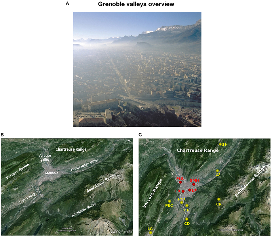
Figure 1. (A) Particulate Matter pollution during wintertime inversions over Grenoble (Photography: courtesy of Eric Chaxel). (B) View of the mountain ranges and Grenoble valleys discussed in the paper. (C) Locations of the ground-based Automatic Weather Stations (yellow) and air-quality stations (red, not used in the present study); the acronyms are defined in Table 1. Extracted and adapted from Largeron and Staquet (2016) with background maps taken from Google Earth.

The ABL in complex terrain during persistent inversions has therefore very specific features compared to the flat ABL, since slope and valley winds control the flow dynamics in the former case. As a result, data stemming from field campaigns or numerical experiments over flat terrain (see Mahrt, 2014; Sun et al., 2015, for a review) cannot be used to get insight into the ABL dynamics in complex terrain.

TABLE 1

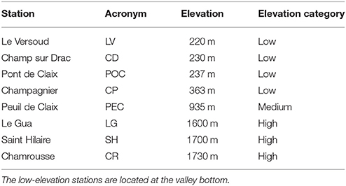
Table 1. Description of the ground-based Automatic Weather Stations in the Grenoble valleys.

Several field campaigns dedicated to the study of persistent inversions in complex terrain have been conducted, with gradual focusing on smaller scales and growing importance of numerical studies for planning and conducting the campaigns and analysing the data. Campaigns were held in the Colorado basin (Wolyn and McKee, 1989; Whiteman et al., 1999a) or Columbia basin (Whiteman et al., 2001; Zhong et al., 2001) and first aimed at studying the formation, stagnation and destruction of the inversions (or cold air pools). Recent programs also include air quality concerns, such as PCAPS (Persistent Cold-Air Pool Study) in the Salt Lake valley (Silcox et al., 2012; Lareau et al., 2013; Wei et al., 2013). In Europe, the COLPEX program (COLd air Pooling and fog formation over complEX terrain), led by the Met Office in the UK, involved field and high-resolution numerical studies in a region of small hills in the UK (Price et al., 2011; Vosper et al., 2014). In the Alps, the first wintertime field campaign aiming at studying persistent inversions was held in the Chamonix-Mont-Blanc valley in January–February 2015, motivated by the anomalously high pollution level frequently recorded there; both meteorological and chemical data were collected during the campaign (Chemel et al., 2016).

In valleys, during persistent inversions, several mechanisms can significantly impact the concentration and the transport of pollutants, among which the slope and valley winds (Gohm et al., 2009). Down- and up-slope winds can drive the spatial distribution of pollutants which can be strongly heterogeneous inside the valley ABL (Schnitzhofer et al., 2007; Harnisch et al., 2009). Interactions between the cold-air pool and the valley winds are frequent (Banta et al., 2004; Cuxart et al., 2007) and the local specificities of a given site need to be investigated to know whether these valley-scale processes can explain the observed evolution of pollutant concentrations.

In France, the city of Grenoble is very critical in terms of pollution due to both its deep and landlocked orography and to the high-occupancy of the territory (Figure 1A): the city counts over half a million inhabitants and many industries. Moreover, the region of Grenoble is a strategic traffic crossroads, as a transit point and a necessary access to many ski resorts. Pollutant emissions, such as PM₁₀ (particulate matter of diameter less than 10 μm) are then important and often concentrated on specific periods which coincides with periods when the boundary layer is the most stable. These emissions thus tend to result in acute episodes of local pollution, which makes Grenoble stand among the most polluted cities in France (Air Rhône-Alpes, 2011). Despite the strong impact of wintertime ABL dynamics on local air quality, field campaigns held in the Grenoble valleys up to now have focused on the summertime ABL to account for ozone pollution (Couach et al., 2003) and on the chemistry of aerosols from urban ground stations (Favez et al., 2010). No wintertime field campaign investigating the ABL dynamics has been performed yet. The present study, mostly numerical, is the first attempt to identify the circulation and thermal structure in the Grenoble valleys during wintertime persistent inversions, thus providing insights into the surface layer ventilation during such events. More details can be found in Largeron (2010). As we shall show, some conclusions of the present study apply to valleys with similar deep and complex orography, implying that they could be generalizable to many other world valleys. In the following, focus is made on the persistent stage of the inversion, between formation and destruction. Time series of 2-m air temperature data recorded at different altitudes around the city, and simulation results from high-resolution mesoscale simulations are used. In this study, we used the MesoNH numerical model (Lafore et al., 1998) that has already been successfully used to model stable ABL (e.g., Cuxart and Jiménez, 2007; Martínez et al., 2010) and valley or basin winds (e.g., Flamant et al., 2002; Cuxart et al., 2007; Drobinski et al., 2007).

In Section 2, we use the temperature data to identify the persistent inversion of the 2006–2007 winter in the Grenoble area. Nine such inversions are identified between November and February, which all coincide with very poor air quality. Numerical simulations of the five longest and strongest persistent inversions are then carried out, to investigate the general flow organization inside the valley and its possible coupling with the free troposphere (Section 3). A detailed study of one such inversion is next conducted, using a higher vertical resolution. Results are reported in Section 4 for the wind pattern and in Section 5 for the thermal structure of the persistent inversion. Conclusions are drawn in Section 6.

2. Detection of Persistent Inversions

2.1. The Grenoble Valleys and the Ground-Based Observations

2.1.1. The Grenoble Valleys

The city of Grenoble is located in the French Alps and lies at the junction of three valleys, the Grésivaudan valley on the north-east, the Voreppe valley in the north-west and the Drac valley in the south (see Figure 1B). These valleys have a width comprised between 3 and 5 km and are of several tens of kilometers long. They separate three mountain ranges, the Vercors range on the west of the city, the Chartreuse range on the north and the Belledonne range on the east part. The highest altitude of the two former ranges is 2000 m ASL (above sea level) while the Belledonne range peaks at 3000 m ASL. The site also involves a fourth valley, the Romanche valley located south-east of Grenoble, which is narrower, deeper and higher in altitude than the other three valleys. The area comprising these four valleys and the city of Grenoble will be referred to as the Grenoble valleys hereafter. The flat part of the valley around and including Grenoble, will be referred to as the Grenoble basin; the largest width of this basin is about 6.5 km, and its altitude is 210 m ASL. The city of Grenoble has severe wintertime PM₁₀ pollution issues. The number of days where the daily-average PM₁₀ concentration exceeds the warning threshold of 50 μg m⁻³ has been of 50 in average per year over the 2007–2010 period, therefore exceeding the threshold of 35 per year set by the French legislation (Air Rhône-Alpes, 2011).

2.1.2. The Ground-Based Observations

The Grenoble valleys are equipped with ground-based Automatic Weather Stations measuring 2-m air temperature, and 10-m wind speed and direction every hour. These stations, which are either routinely operated by Meteo-France, the French weather forecast service, or by Air Rhône-Alpes, the air quality agency of Région Rhône-Alpes, are located at different places and altitudes in the Grenoble valleys. Time series of the temperature at eight stations have been used for the present study, whose name and elevations are displayed in Table 1, and locations indicated in Figure 1C. As can be seen from Table 1, the stations can be broadly categorized as low elevation, medium elevation and high elevation stations.

2.2. Methodology

We developed a simple method to detect persistent inversions of the 2006–2007 winter using the temperature records from the eight ground-based meteorological stations listed in Table 1. The principle of this method, detailed in Largeron and Staquet (2016), is to compute a bulk measure of the stability of the ABL from which persistent inversions are detected when this bulk measure exceeds a given threshold.

Figure 2A displays the 2-m air temperature recorded at the stations LV and CR during the month of December. Two points should be noticed: (i) the temperature difference between these two stations exhibits a high variability over the month; (ii) two main persistent inversion episodes occur, around mid-december and at the end of the month, during which the temperature at the valley bottom can be lower by 10 K than that at the high-elevation station.

FIGURE 2

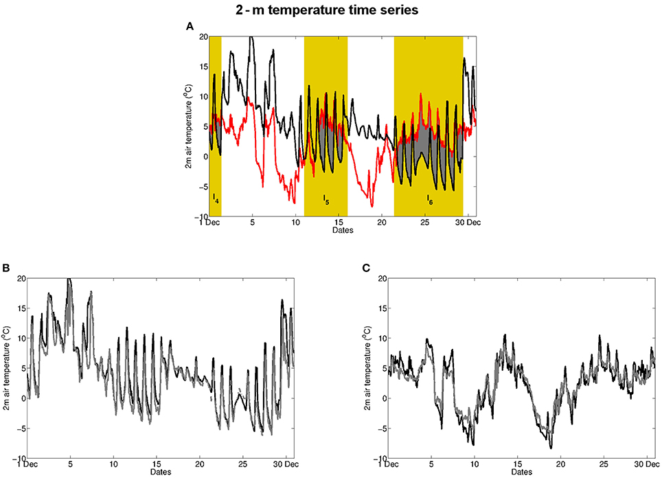
Figure 2. Time series of 2-m air temperature in December 2006 at (A) the low-elevation station of LV (black) and the high-elevation station of CR (red). The gray-shaded zones refer to temperature inversions (the temperature in CR is higher than in LV); persistent inversions defined by criterion (1) are indicated by a yellow veil; (B) two low-elevation stations, LV (black) and POC (gray); (C) two high-elevation stations, CR (black) and LG (gray).

Inside the valley ABL, temperature records show that the temperature field is approximately horizontally homogeneous. Temperature time series at stations of similar elevations are indeed strongly correlated (r² = 0.97), as can be seen for the two low-elevation stations of LV and POC (Figure 2B), or similarly for the two high-elevations stations of CR and LG (Figure 2C), for the whole month of December. On the opposite, high-elevation stations display a very distinct behavior than low-elevation stations (see Figure 2A) with a low correlation (r² = 0.36). It can be shown that the temperature difference between two stations belonging to the same category is two orders of magnitude smaller than the temperature difference between a high- and a low-elevation station, on average over the five considered months (November 2006 to March 2007). It follows that the temperature difference between the top and the bottom of the ABL is well estimated by the difference in temperature between any high-elevation station and any low-elevation station, and that the latter may be indicative of the ABL static stability. This is consistent with the results of Whiteman et al. (2004) who have shown that temperature vertical profiles can be well-approximated by pseudovertical profiles obtained from temperature stations on the sidewalls, in strongly stable and low synoptic wind conditions.

In valleys, inversion layers often fill the entire ABL up to the valley top (Whiteman, 1982). In the present case, the valley top is about 1500 m, which implies that the high-elevation stations are located just above the inversion. As shown below, this statement is consistent with results from numerical simulations of the Grenoble valleys.

A persistent inversion can therefore be detected by considering the temperature difference between a high- and a low-elevation station, divided by their elevation difference, (ΔT/Δz)_i, where the index i refers to any couple of stations. We compute the average over 4 such couples of stations of the temperature difference across the ABL, which we refer as the bulk temperature gradient hereafter and denote ΔT/Δz.

The detection of persistent inversions is then made using the following criterion:

$\begin{array}{l}{\langle \Delta T/\Delta z\rangle }_{24\text{ h}}>{\langle \Delta T/\Delta z\rangle }_{\text{winter}}\text{ for more than }72\text{ consecutive}\\ \text{ hours}& (1)\end{array}$

where < >_{24 h} and < >_winter represent a 24-h-running average and the winter average (from November to March), respectively. For the winter of 2006–2007, < ΔT/Δz > _winter is about −3 K.

The 24-h-running average bulk temperature gradient < ΔT/Δz > _{24 h} is displayed over the whole winter in Figure 3, along with the constant value of −3 K. Using criterion (1), nine persistent inversions are detected, which are referred to as I_k, 1 ≤ k ≤ 9. The December inversions are also indicated in Figure 2A. The characteristics of these nine inversions are displayed in Table 2, namely their period of occurrence with respect to criterion (1), the corresponding duration and an estimate of their strength as measured by the bulk temperature gradient averaged over their respective duration. The longest and strongest inversion is I₆, on which we shall mainly focus in the following.

FIGURE 3

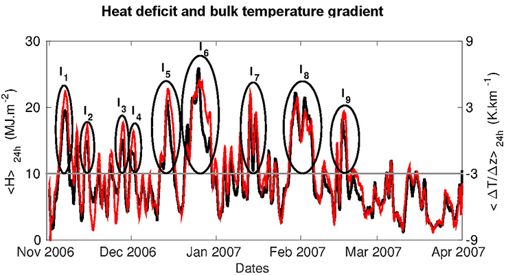
Figure 3. Temporal evolution of the 24-h-running average of the bulk temperature gradient ΔT/Δz (red) and heat deficit H (black) during the 2006–2007 winter. The 9 inversions I_k, 1 ≤ k ≤ 9, detected by criterion (1) are circled in black. The persistence threshold < ΔT/Δz > _winter is indicated with a gray line. Extracted and adapted from Largeron and Staquet (2016).

TABLE 2

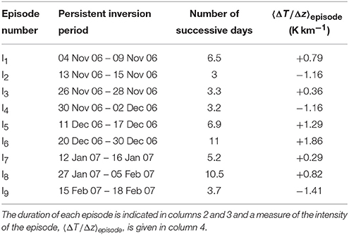
Table 2. Persistent inversions detected using criterion (1).

Criterion (1) can be equivalently expressed in terms of the heat deficit H inside the inversion layer (Largeron and Staquet, 2016). The heat deficit is the amount of heat which should be provided to bring the temperature gradient to the adiabatic gradient, namely to fully mix the fluid column (Whiteman et al., 1999a,b). The 24-h-running average of the heat deficit is also displayed in Figure 3. As shown in this figure, the −3 K threshold for the winter-average bulk temperature gradient is equivalent to a threshold value of 10 MJ m⁻² for the winter-average heat deficit.

It can also be shown (Largeron and Staquet, 2016) that (i) the nine detected episodes are strongly polluted, in the sense that the 24-h-running average concentration of PM₁₀ exceeds the air-quality legal threshold of 50 μg m⁻³ for at least three consecutive days during each episode; (ii) all persistent inversion periods reported in Table 2 occur during and are triggered by anticyclonic conditions; (iii) all persistent inversions are generated by a mid-level warming and destroyed by a mid-level cooling.

3. The Nocturnal Wind Circulation in the Grenoble Valleys During Persistent Inversions

Figure 3 and Table 2 show that, among the nine persistent inversions of the considered winter, four of them (I₂, I₃, I₄, and I₉) last for a short duration (though greater than 3 days) and are of lower intensity. On the opposite, the five other persistent inversions last longer and are associated to stronger inversion strengths. These five episodes all involve a stagnation stage (see Largeron and Staquet, 2016), between the formation and the destruction of the inversion, during which the inversion displays similar features from one day to the next. The stagnation stage will also be referred to as the heart of the episode hereafter. In the following, focus is made on these five episodes for which numerical simulations are made, in order to investigate the main characteristics of the wind circulation in the Grenoble valleys during persistent inversions. We briefly describe the numerical model below, stressing the aspects relevant to the present study, before analyzing the wind circulation in the valleys. More details are provided in Largeron (2010).

3.1. Description of the Numerical Simulations

We performed high-resolution mesoscale simulations (according to the terminology defined by Cuxart, 2015) of the five episodes I₁, I₅, I₆, I₇, and I₈ using the Meso-NH numerical model developed by Meteo-France and the Laboratory of Aerology (Lafore et al., 1998).

The numerical model Meso-NH solves the Navier-Stokes equations in the anelastic approximation, thus filtering sound waves while allowing the density to vary in space and time. The model uses a terrain-following coordinate system along the vertical direction. The atmospheric model is coupled with the externalized land and ocean surface model SURFEX (Masson et al., 2013), to account for the surface fluxes and the evolution of four types of surfaces: nature, town, inland water and ocean with a large variety of ground covers. It can include a specific parameterization scheme for the urban energy budget (Masson, 2000). A full three-dimensional turbulence scheme that uses a prognostic equation for the turbulent kinetic energy is activated (Cuxart et al., 2000). The model may also include microphysical schemes for mixed-phase clouds and warm clouds and other specific parameterization for chemical species and aerosols, which we did not use in the present study.

As is now standard, a nesting of domains is used, allowing to capture the dynamical features of a wide range of scales and to focus on small scale processes in the innermost domain, which has the highest resolution (e.g., Zhou and Chow, 2013). The vertical resolution in each domain is the same, the size of the horizontal grid cells being decreased -in the present case by a factor of 3- from one outer domain to the inner one. For the present study, four nested domains are used, which are all centered on the Grenoble valleys. The largest domain D₁ has a horizontal resolution of 9 km and an extension of 675 × 675 km; and is forced at the boundary with 6-hourly fields from ECMWF operational analyses. The innermost domain is of size 30 × 30 km, with a horizontal grid size of 0.333 km. The databases Gtopo30 for the orography, with a resolution of approximately 1 km, and Ecoclimap 2 (Masson et al., 2003) for the ground cover are used, and are interpolated in the innermost domain to 1/3 km. Two configurations are considered, denoted C₁ and C₂ in Table 3 below, which mainly differ in the vertical resolution and duration of the computation. In configuration C₁, 60 levels are used in all domains, the vertical resolution at the ground being 15 m. In configuration C₂, a finer vertical resolution is used, of 4 m close to the ground, with 90 levels in total. The grid size is stretched along the vertical, the resolution being equal to 600 m at the top of the domain in each configuration. The duration of the computation is 10 h in C₁ and 53 h in C₂. The main features of the simulations are summarized in Table 3. The influence of these numerical choices (vertical resolutions and duration of the simulations) is investigated in the following Section 3.2 and in the Supplementary Material.

TABLE 3

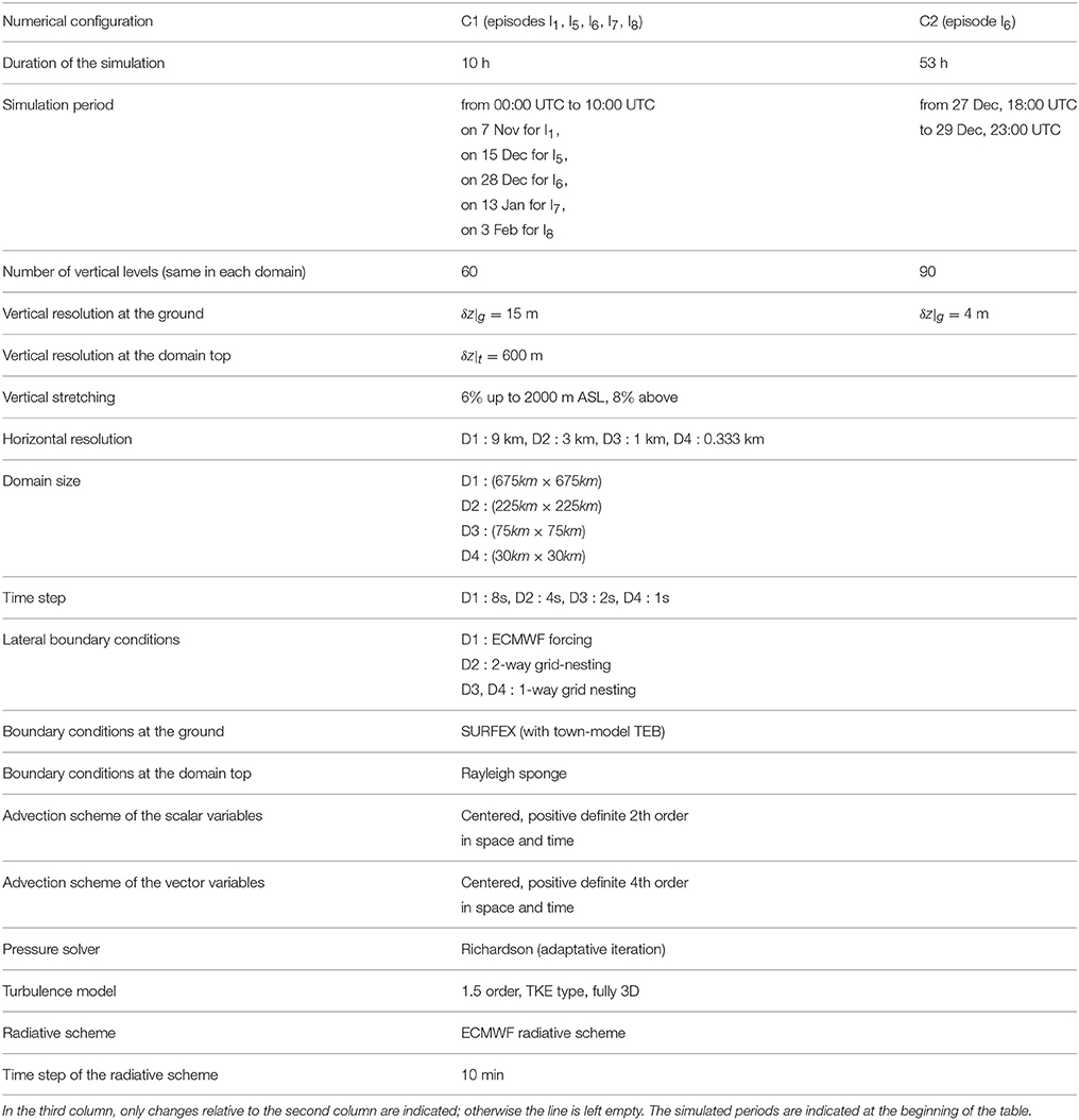
Table 3. Main parameters of the numerical simulations.

3.2. Sensitivity Analysis of the Numerical Simulations

A first sensivity analysis has been made to investigate the numerical spin-up in the case of episode I₆ and configuration C₁. Starting the run at different times (0 h UTC on December 27, 18 h UTC on December 27 and 0 h UTC on December 28), results were compared at the end of the night (06:00 UTC) on December 28. This test, which is not presented here, leads to the conclusion that the numerical spin-up is about 4 h, namely, if comparison is made at the same time at least 4 h after the beginning of all the simulations, then the temperature and wind fields inside the valley are similar (see Largeron, 2010, for details). This result shows that the nocturnal quasi-steady circulation at valley-scale at the end of the night and in early morning (on which we focus in the following Section 3.3) can be analyzed by means of simulations starting at 0 h UTC in the C1 configuration. This choice appears facilitated by the presence of a persistent inversion which implies that an elevated inversion is already present and seen by the outer domain at the beginning of the simulations at 0 h UTC.

A second sensitivity analysis has been performed to investigate the effect of the vertical resolution, in the case of episode I₆, during the night from 18 h UTC on December 27 to 8 h UTC on December 28. This analysis is reported in the Supplementary Material. The main conclusion is that the vertical resolution close to the ground should be at least δz|_g = 15 m for the general features of the ABL dynamics and temperature profiles to have converged. Hence, a vertical resolution of δz|_g = 15 m can therefore be considered as sufficient to model these features.

However, comparisons with ground observations of 2-m air temperature data show that in a very shallow layer close to the ground, the temperature is only well reproduced with a fine resolution of δz|_g = 4 m in high-elevation stations, and still has a hot bias at the low-elevation stations.

For δz|_g > 4 m, simulations present a systematic hot bias at the bottom of the valley, and a systematic cold bias in altitude, which otherwise formulated, corresponds to a too weak temperature inversion compared to the observations. In this case (δz|_g > 4 m), surface fluxes suffer from a misrepresentation that in turn leads to a too weak cooling of the near-surface air in altitude and to an underestimated drainage of cold-air by katabatic winds toward the bottom of the valley.

In the following, consistently with these findings, the analysis made with the C₁ configuration (δz|_g = 15 m) then only deals with the general ABL dynamics for which a finest resolution leads to the same results. Fine-scale details of the near-surface ventilation and temperature gradient, reported in Sections 4 and 5, rely on the C₂ configuration (δz|_g = 4 m) instead.

3.3. Overall Nocturnal Circulation of the Five Episodes

Focus is made on one night of the five episodes I₁, I₅, I₆, I₇, and I₈, each simulation starting at 00:00 UTC and lasting for 10 h (see configuration C1 in Table 3). These nights are indicated in Table 3.

3.3.1. Synoptic Regime

As noted at the end of Section 2, each episode occurs under anticyclonic conditions, with low synoptic wind speed, of about 4 to 5 m s⁻¹. As for the wind direction, taken at the 600 hPa geopotential height (which is about 4200 m ASL in the present case of strong anticyclone), it hardly varies over the 10 h of the simulation but varies from one episode to the other: it flows either from the south–east (I₁, I₅), north–west (I₆), west (I₇) or from the east (I₈). The synoptic regime during each simulated period is very stable, the altitude of the 600-hPa geopotential height over the area varying by less than 15 m for I₁, I₆, I₇, I₈ and by 35 m for I₅.

These features of the synoptic wind computed by the model are consistent with those recorded from radio-soundings at the Lyon Saint Exupery airport, located about 80 km from the Grenoble site, which is a small distance compared to the synoptic scale. Wind recorded over 3000 m ASL there, the altitude of the highest summits of the Grenoble area, is representative of the synoptic wind over this site.

3.3.2. Valley Wind Circulation at the End of the Night

The key feature of the valley-scale circulation in the Grenoble valleys is that it consists in the superposition of several valley winds flowing from the different mountain ranges and valleys of the site. This circulation slightly varies from one episode to the other but common dominant features can be extracted, which are illustrated in Figure 4 by maps of the wind vector field at different altitudes between 350 and 3000 m ASL, for episode I₆. A sketch of this circulation is displayed in Figure 5 for each of the five episodes.

FIGURE 4

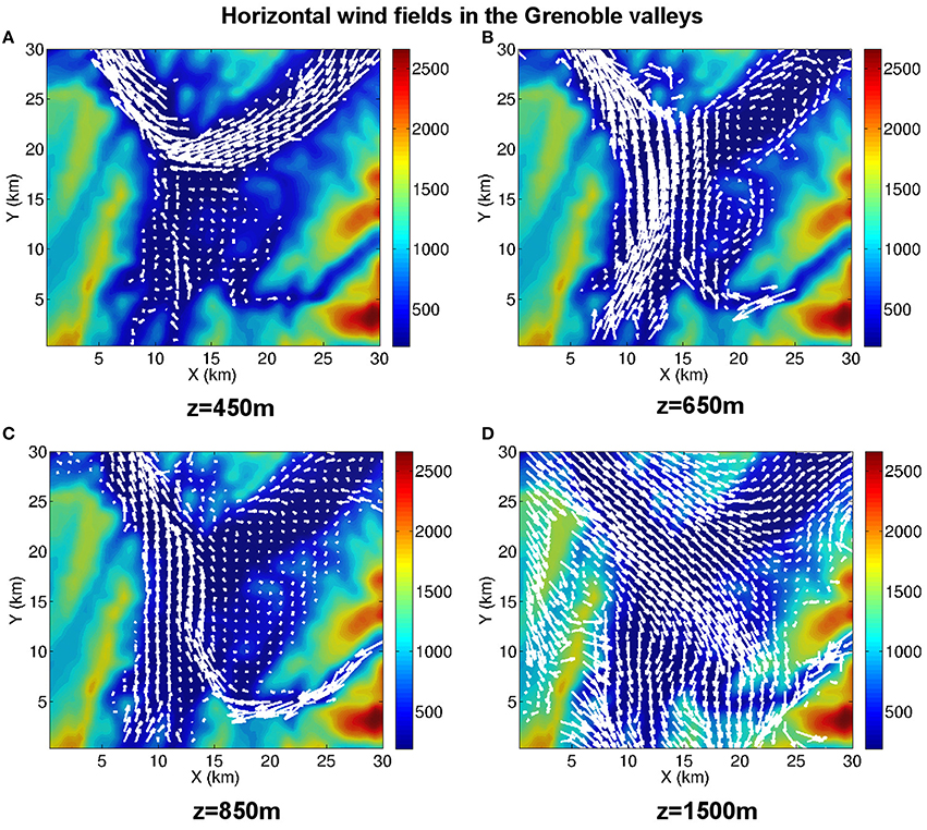
Figure 4. Maps of the wind at a given altitude during episode I₆ at 06:00 UTC on December 28. (A) z = 450 m ASL; (B) z = 650 m ASL; (C) z = 850 m ASL; (D) z = 1500 m ASL.

FIGURE 5

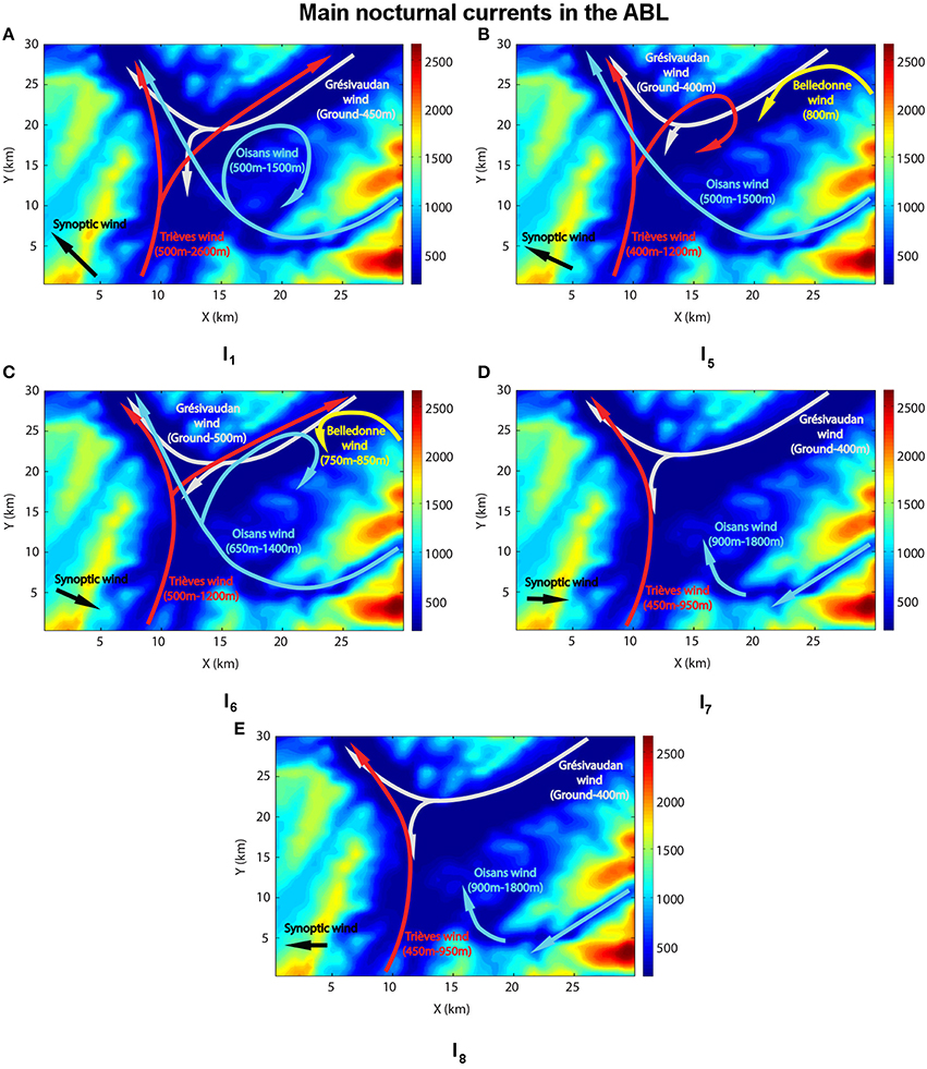
Figure 5. Sketch of the main nocturnal currents during the heart of episode. (A) I₁ (November 7); (B) I₅ (December 15); (C) I₆ (December 28); (D) I₇ (January 13); (E) I₈ (February 3).

During these five episodes, the circulation in the Grenoble valleys consists in four main winds which flow almost horizontally at different altitudes, resulting in a vertical layering in the ABL:

• The Grésivaudan wind flows along the bottom of the Grésivaudan valley from the north-east (the Grésivaudan valley has a very gentle slope descending toward Grenoble). This is a cold wind, which extends vertically over a layer of thickness 150–250 m, namely between the ground and about 500 m ASL (as shown in Section 4). It splits into two mass fluxes over the city, the major part flowing into the Voreppe valley toward the north-west, while a smaller part flows southward (Figure 4A and white colour current in Figure 5).

• The second wind comes from the Trieves plateau located south of Grenoble (Figure 4B and red colour current in Figure 5). We refer to this wind as the Trieves wind. It flows between about 500 m ASL, therefore above the Grésivaudan wind, to an altitude of 1000 to 1200 m ASL depending upon the episode. This wind is then channelled into the Voreppe valley whatever the episode. A small part flows into the Grésivaudan valley for episodes I₁ and I₆, in the direction opposite to that wind (and above it), while it recirculates as a large scale vortex over the city in I₅ (Figure 4B). A smaller vortex structure also forms along the flank of the Belledonne range, between 500 and 700 m ASL (as is visible in Figure 4B).

• The third wind flows from the Romanche valley and reaches the Grenoble basin from the south-east (Figure 4C and blue color current in Figure 5). This cold wind, referred to as the Oisans wind, meets the Trieves wind over the city between 600 and 1000 m ASL. A part of the mass flux is then channeled into the Voreppe valley and flows along with the Trieves wind (I₁, I₅, I₆). Another part recirculates as a large-scale vortex in the Grenoble basin and in the Grésivaudan valley (I₁, I₆). The thickness of the Oisans wind varies from one episode to the other, ranging from 500 and 1800 m ASL, which are roughly the lowest and highest altitude of the Romanche valley, respectively.

• Between 750 and 850 m ASL, a fourth wind, the Belledonne wind is sometimes observed (I₅ and I₆), which flows from the Belledonne range into the Grésivaudan valley while oscillating. Several large scale vortex structures are then visible in the latter valley.

From 1500 m ASL, which is the inversion altitude, up to 2500–3000 m ASL, the circulation appears to result from the channelling of the synoptic wind into the valleys. For episode I₆ (Figure 4D), this wind comes from the north–west in this range of altitudes. It is noticeable that this direction is opposed to, or at least very different from, that of the four winds just described, which flow below 1500 m ASL.

It appears from the five simulations that these local dynamics set in during a persistent inversion below 1500 m ASL, and are almost independent of the episode. The circulation inside the Grenoble valley can be decomposed into four winds, which are all associated with along-valley winds flowing almost horizontally at different altitudes, resulting in a vertical layering of the ABL. Large-scale vortices also form over the entrance of the Grésivaudan valley and along the flank of the Belledonne range.

3.3.3. Influence of the Synoptic Wind

Following Whiteman and Doran (1993), the direction of the wind in the Grésivaudan and Voreppe valleys is plotted vs. the direction of the synoptic wind for all five episodes in Figure 6. More precisely, for the Grésivaudan wind, an average of the wind direction from the ground to an altitude of 400 m ASL on all grid points of this valley is computed every hour of the simulated episode (see Table 3). The same average is applied to compute the Voreppe wind direction, the points considered being now in the Voreppe valley, from the ground to an altitude of 600 m ASL. These grid points are indicated in Figure 7A.

FIGURE 6

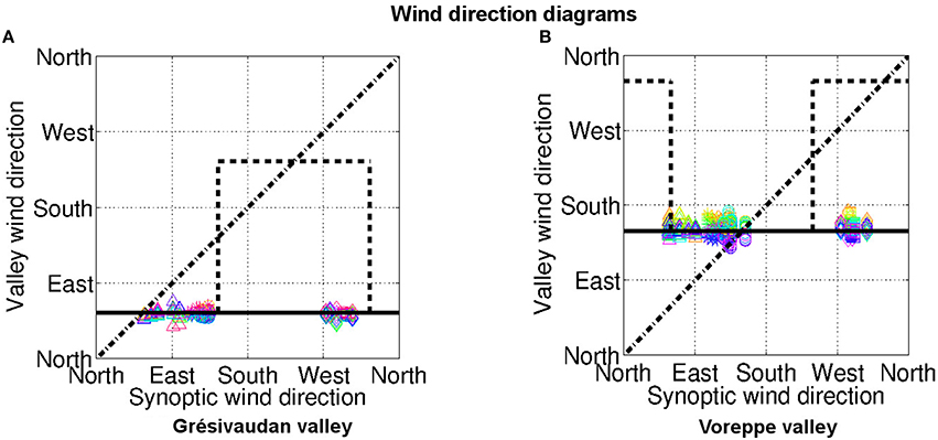
Figure 6. Direction of the valley-wind vs. that of the synoptic wind. The valley-wind direction is plotted every hour of the C1 configuration, each hour having a different color, and each episode is represented by a symbol: ◦: I₁, ⋆: I₅, □ : I₆, ◇: I₇, △: I₈. The horizontal black line is the direction of the valley close to the Grenoble basin. (A) Grésivaudan valley; (B) Voreppe valley. The valley-wind direction is averaged over the horizontal grid points displayed in Figure 7A, from the ground up to 400 m for the Grésivaudant valley and up to 600 m for the Voreppe valley. See text for details.

FIGURE 7

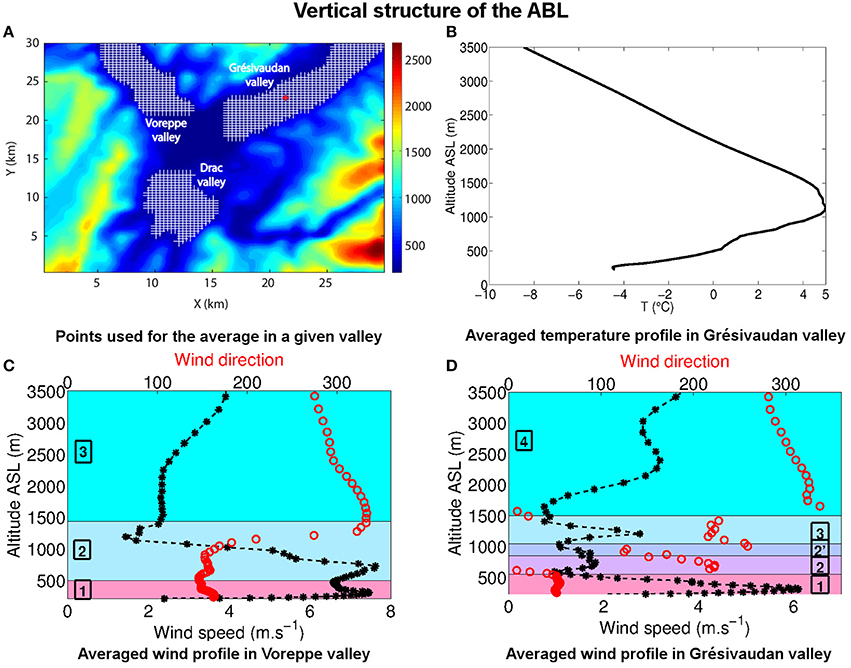
Figure 7. (A) The hatched zones are those over which the average for the Voreppe valley, the Grésivaudan valley and the Drac valley are performed. The point Gr, referred to in Section 5, is indicated with a red + symbol. (B) Vertical profile of temperature averaged over the Grésivaudan valley. (C) Vertical profile of wind speed (⋆) and wind direction (◦) averaged over the Voreppe valley. (D) Same as (C) in the Grésivaudan valley. The averages are performed over the horizontal grid points displayed in frame (A). Profiles are shown at 06:00 UTC on December 28.

Figure 6 clearly shows that the wind keeps the same direction in either valley whatever the episode and, therefore, whatever the synoptic wind direction. For the Voreppe valley and episode I₆ for instance, the valley-wind flows toward the north–west, namely in the opposite direction to the synoptic wind. The same decoupling with the synoptic wind is observed for the Drac and Romanche valleys (not shown). This allows us to conclude that these winds are of thermal origin and result from the radiative cooling of the ground in a complex topography.

Note that the other processes leading to the formation of winds in the ABL, discussed by Whiteman and Doran (1993), are very unlikely and would have another signature. Indeed, a downward transport of horizontal momentum from above the valley, which would rather occur under unstable or neutrally stable conditions, would result in a linear dependency between the valley-wind direction and synoptic-wind direction (as indicated by the dashed dotted line in Figure 6). The channeling of the synoptic wind into the valleys (for a strong enough wind for instance) would lead to a step function (dashed line in Figure 6).

It follows that, during a wintertime persistent inversion, a unique organization of the valley-scale circulation within the Grenoble valleys sets in in the ABL, which does not depend upon the episode, because it is decoupled from the synoptic wind. This circulation is controlled by the local topography and the radiative cooling of the ground. Hence, a single episode may be considered as being representative of any persistent inversion of the winter when the circulation in the valley is considered.

4. Spatial Structure of the Atmospheric Boundary Layer

In the following focus is made on the heart of episode I₆, simulated with the finest resolution of the C₂ numerical configuration and for a longer period of 2 days (see Table 3).

The choice of episode I₆ results from several considerations:

• I₆ is the strongest and the longest persistent inversion of the considered winter (see Table 2).

• The heart of episode I₆ is associated with a very low synoptic wind which flows from the north-west, namely in the direction opposite to most thermal winds of the Grenoble valleys, thereby waiving any doubt on the physical origin of the latter winds.

• The valley-scale circulation in the Grenoble valleys during episode I₆ is representative of the circulation during the other simulated episodes. This episode also clearly reveals the presence of the Belledonne wind, which is weaker in the other episodes.

4.1. Vertical Structure of the Nocturnal Winds

Vertical profiles of the wind speed and direction are displayed in Figure 7 for the Voreppe valley (Figure 7C) and for the Grésivaudan valley (Figure 7D). Results are shown at the end of the night (06:00 UTC) and are representative of the nocturnal vertical structure of the wind during the heart of the episode. The wind field is horizontally averaged over grid cells of the considered valley (displayed in Figure 7A) and the resulting mean speed and mean direction are computed as a function of altitude. The averaged vertical temperature for the Grésivaudan valley is also displayed in Figure 7B.

Figure 7D yields a refined view of the vertical layering described in the previous section for the Grésivaudan valley:

• The first layer (numbered as 1 in Figure 7D) lies above the ground (at about 220 m ASL), up to ≃500 m ASL, and is associated with the Grésivaudan wind. This wind blows from the north-east and is of rather large amplitude, up to 6 m s⁻¹ reached at about 300 m ASL. Figure 7B shows that this layer is strongly stable, the average vertical potential temperature gradient $\partial \overline{\theta }/\partial z$ being equal to 22 K km⁻¹ in the layer.

• The second layer (numbered as 2 in Figure 7D) surmounts layer 1 and is associated with a mean mass flux from the south-west, which is therefore up-valley and opposed in direction to the Grésivaudan valley. This layer is associated with the Trièves and Oisans winds which overlap in this range of altitudes. The layer is very inhomogeneous horizontally as it involves large scale vortices (of size close to half the valley width). The wind direction therefore strongly varies, implying a weak average wind speed. Like layer 1, layer 2 is strongly stable ($\partial \overline{\theta }/\partial z\simeq$ 21 K km⁻¹).

• An intermediate layer (denoted as 2') may be noticed between 800 and 950 m, which corresponds to the Belledonne wind. The mass flux flows here from the Belledonne to the Chartreuse range, with a direction comprised between 120 and 170° (namely from the south-east). This wind is weak, of less than 2 m s⁻¹.

• In layer 3, the mean mass flux is associated with the Trièves wind, blowing from the south-west. It has a clear jet type structure, with maximum value of about 2.7 m s⁻¹ reached at 1250 m. This layer extends from about 1000 to 1500 m and is stable with a nearly uniform temperature (corresponding to $\partial \overline{\theta }/\partial z\simeq$ 10 K km⁻¹).

• Finally, the fourth layer (number 4 in Figure 7D) may be considered as a buffer zone between the top of the inversion layer and the bottom of the free troposphere. The synoptic wind is recognized here, being orographically channelled. It flows from the north-west with a slightly veering direction with altitude due to the shape of the mountain ranges. The stability of this layer is weaker, with $\partial \overline{\theta }/\partial z\simeq$ 3.6 K km⁻¹, which is that of the free troposphere above.

The complex wind structure in the Grésivaudan valley, where the signature of the different winds can still be clearly recognized, contrasts with that in the Voreppe valley displayed in Figure 7C. There, only three main layers can be distinguished, the lowest two layers being associated with thermal winds channelled into this valley (toward the north-west) after their coming out in the Grenoble basin. The first layer corresponds to the Grésivaudan wind, up to 500 m ASL. The second layer, from 500 m to about 1100 m, results from the overlapping of the Trieves and Oisans winds (locally a third maximum can be observed around 1000 m, associated with the Oisans wind). The maxima of these jets reach a higher value than in the Grésivaudan valley, of 7.5 m s⁻¹, due a strong pressure gradient between the Grenoble basin and the plain located northwest of the Voreppe valley, which accelerates the wind (not shown). The wind direction veers above 1000 m to align with that of the synoptic wind, marking the beginning of the buffer zone, which forms the third layer.

The Voreppe valley thus plays an important role in the ventilation of the Grenoble basin, in draining away the thermal winds. The air masses associated with these winds would otherwise partly accumulate in the Grenoble basin, possibly leading to an even higher pollution level during these wintertime persistent inversions.

The thermal winds and cooling of the ground at the bottom of the valley shape the temperature field, once anticyclonic conditions have set in. As a result, an inversion layer develops from the ground up to 1500 m, close to the altitude of the valley top as discussed in Section 2. Figure 7B thus shows that the mean temperature profile is nearly linear, the mean temperature at a height of 1000 m above the valley bottom being almost 10°C higher than at the bottom. The temporal evolution of this profile and associated structure of the inversion layer are analyzed further in Section 5.

4.2. Diurnal Circulation

On December 28 at the latitude of Grenoble, the astronomical sunrise is at 07:18 UTC, the sunset being at 16:02 UTC. Due to orographic shading, the local sunrise is delayed by 1 h in the major part of the valley bottom, and similarly, the local sunset is advanced by about 1 h in most of the Voreppe and Drac valley (but this is not the case in the Grésivaudan valley, which has an almost full sky view factor in the west direction, and is therefore not significantly shaded in the late afternoon by the Vercors range located westward). In the Grenoble basin, whereas the duration of the day is theoretically of 8h45, the duration of the period with a positive incoming insolation is then reduced to about 6h45. This implies that the diurnal cycle is dominated by its nocturnal component, which lasts almost 18 h.

Moreover, as will be shown in Section 5, due to both the low value of the wintertime insolation (further reduced by the orographic shading) and the strong stability over a significant depth of the inversion layer, daytime warming only affects a very shallow layer from the ground up to about 50 m above it. In this shallow layer, daytime convection occurs and triggers an up-valley wind in the main valleys of the site (not shown). The upper layers of the ABL, from 50 m above the ground up to the inversion top, are not affected by the daytime warming and the valley-scale circulation herein remains the same as during nighttime.

Consequently, on a diurnal cycle, the valley-scale circulation inside the ABL is dominated by the nighttime valley winds detailed in the previous section. This nighttime wind organization indeed prevails in all the ABL during the cooling stage (from about 15:00 UTC to 09:00 UTC), and above the shallow convective layer of thickness 50 m during the warming stage (from about 09:00 UTC to 15:00 UTC).

The nocturnal wind circulation described in Section 4.1 can therefore be considered as representative of the ABL kinematic structure all along the heart of a persistent inversion.

4.3. Recirculation and Stagnation Areas in the Grenoble Valleys

In this section, focus is made on the first 50 m above the ground in order to analyse the ventilation of the surface layer. The main motivation is to determine the areas where no ventilation occurs, referred to as stagnation areas, which have an increased impact on air quality and human health. For this purpose, we use the quantification method developed by Allwine and Whiteman (1994) for the Colorado plateau basin. This method relies on two indices, a stagnation index S and a recirculation index R, which are defined from the knowledge of the horizontal wind field components. The stagnation index, computed between two instants t₀ and t₁, represents the distance travelled by a fluid particle during this time interval. The recirculation index is also built with the wind field components, and with the stagnation index and takes values between 0 and 1: for R = 0, the fluid particle does not recirculate while for R = 1, the fluid particle exactly returns to its t₀-position at t₁. Allwine and Whiteman (1994) further introduce critical thresholds from which they define the state of the flow around a measurement station to be in a stagnation, recirculation or a ventilation state. The stagnation state is defined by S ≤ 130 km, the recirculation state by R ≥ 0.6 and the ventilation state by the two conditions S ≥ 250 km and R ≤ 0.2. Of course, the lower and upper bounds for S depend on the wind speed. This method has been used by numerous authors, both for in situ measurements (f.i., Venegas and Mazzeo, 1999) and numerical modeling (f.i., Levy et al., 2009).

The indices S and R have been computed for configuration C₂ in all points of the boundary layer. Averaging the indices over the first 50 m above the ground and over the 2 days of the simulation yields the maps of Figure 8, which displays the stagnation index in Figure 8A and the recirculation index in Figure 8B. Well-ventilated areas appear, which are the Voreppe valley, the Romanche valley and, to a lesser extent, the Grésivaudan valley. By contrast the Drac valley, the south-east of the Grenoble basin, and the flank of the east-face of the Chartreuse range, for which both S ≤ 130 km and R ≥ 0.6, appears as very critical areas for both stagnation and recirculation and, therefore, for the trapping of pollutants which would be emitted there. These results are consistent with the very weak wind field in the Drac valley shown on Figure 4A and with the persistent vortex structure which is present over the south-east of the Grenoble basin as shown on Figure 4B.

FIGURE 8

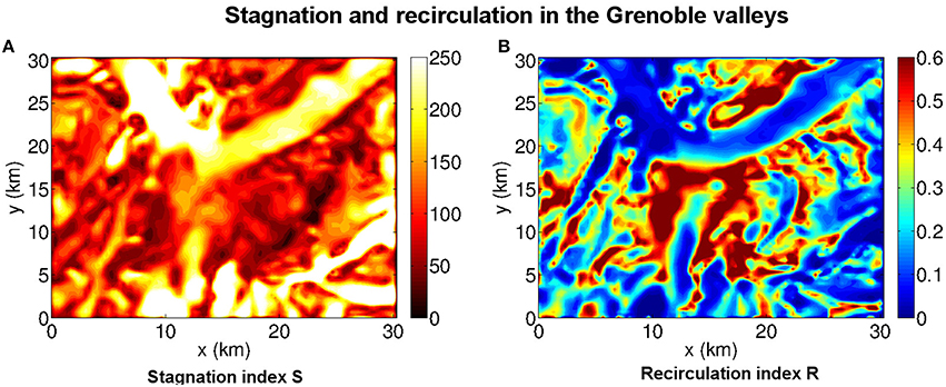
Figure 8. (A) Stagnation index S (in km) averaged over the first 50 m above the ground and over the 2 days of configuration C2. Stagnation areas appear in red and black. (B) Recirulation index R averaged as S. Recirculation areas appear in dark red. Ventilated areas (S ≥ 250 km, R ≤ 0.2) correspond to areas where S appears in white and R in blue.

5. Analysis of the Temperature Inversion During the Stagnation Stage of a Persistent Inversion Episode

5.1. Overall Evolution of a Persistent Episode

As discussed in the Introduction, the formation of the wintertime persistent inversion is controlled by the arrival of a warm air mass at mid-altitude (around 1500 m ASL), associated with very low wind speed; as shown in Section 3, the circulation of the air layer below becomes decoupled from the synoptic circulation and controlled by the thermal winds. The combined effect of cold air advected toward the bottom of the valley by the down-slope and valley winds and of radiative cooling leads to the progressive built-up of an inversion layer, the temperature gradient changing from adiabatic (and therefore negative) values to positive values in a day or two. As shown in Section 4, the inversion layer eventually fills up the whole valley, up to an altitude close to the top of the valley. This evolution is described in details in Largeron and Staquet (2016) and is similar to the one reported by Whiteman et al. (1999a) for the Colorado basin and by Reeves and Stensrud (2009) for valleys and basins in the Western United States.

The destruction of the inversion occurs when a cold front or trough, associated with strong winds and often with precipitation, reaches the region. The lower part of the atmospheric boundary layer becomes affected by the penetration of channelled winds which disturb and eventually destroy the inversion. This process is much more rapid than the formation of the inversion, as it involves mechanical and turbulent mixing processes, as opposed to the built-up of the inversion which results from radiative processes (Largeron and Staquet, 2016).

In the following, we focus on the thermal structure of the inversion during the stagnation stage of episode I₆. All results are shown at one point of the Grésivaudan valley, displayed in Figure 7A, and denoted as point Gr. This point, and the temperature profiles along the vertical line going through it, appear to be representative of the properties of the temperature field in the Grésivaudan valley.

5.2. Diurnal Forcing of the Atmospheric Boundary Layer

In numerical models, the balance of the surfaces fluxes is usually expressed as

$\begin{array}{ll}{R}_n-G-LE-H=0,& (2)\end{array}$

where R_n is the net incoming radiative flux, G the incoming heat flux into the ground, LE the latent heat flux and H the sensible heat flux (f.i., Stull, 1988).

In the SURFEX model, the surface temperature T_s obeys the equation (Noilhan and Planton, 1989)

$\begin{array}{ll}\frac{\partial T_s}{\partial t}=C_T(R_n-LE-H),& (3)\end{array}$

where C_T is the heat capacity of the ground.

The four fluxes R_n, L_E, H and G are plotted vs. time in Figure 9A from 27 December 18:00 UTC to 29 December 20:00 UTC. The dashed lines correspond to the astronomical sunrise and sunset times (without taking into account orographic shading). In the context of the present study, no measurement of the surface fluxes are available so that the model performance can not be explicitly evaluated. Moreover, imbalances are frequently found in observations (e.g., Cuxart et al., 2015), pointing out some conceptual issues concerning the physical parameterizations of surface-atmosphere interactions currently used in numerical models (Foken, 2008). Nevertheless, simulated values suggest that:

• The sensible heat flux and the latent heat flux are much smaller than the radiative flux during both daytime and nighttime;

• The sensible heat flux decreases throughout the night and becomes more and more important as the night advances, whereas the latent heat flux remains negligible all night long;

• The surface flux balance is dominated by the radiative flux during the day and in the first part of the night; but in the second part of the night (after 23 h UTC), turbulence becomes a non-negligible component of the energy budget and partly compensates the long-wave outcoming radiative cooling.

• A radiative warming of the ground occurs for a short period of time, between about 09:00 UTC and 15:00 UTC, the radiative cooling therefore extending over the rest of the day for about 18 h.

FIGURE 9

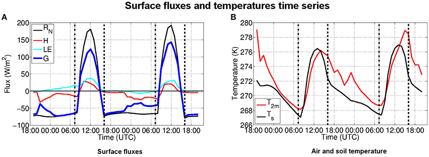
Figure 9. (A) Temporal evolution of the surface fluxes R_N, H, LE, G = R_N−H−LE from 27 December, 18:00 UTC to 29 December, 20:00 UTC in the Grésivaudan valley at point Gr displayed in Figure 7A. The vertical dashed lines are the astronomical sunset and sunrise times for Grenoble. (B) Temporal evolution of the surface temperature (T_s) and the 2-m air temperature (T_2m).

The surface and 2-m air temperature responses are displayed in Figure 9B. The temperatures start to increase shortly after sunrise, up to about noon, consistent with the behavior of the radiative and sensible heat fluxes. A continuous decrease follows during the afternoon and night up to sunrise. These two stages will be referred to as the warming and the cooling stages hereafter.

5.3. Diurnal Evolution of the Inversion

Inversions layers are characterized by their height h_i and their strength Δθ, where θ is the potential temperature, but also by their valley heat deficit (Whiteman et al., 1999a), already referred to in Section 2.2, which corresponds to the heat required to destroy the inversion. If a linear vertical profile of θ is assumed, and if the density ρ and the specific heat of air c_p are assumed to be constant, it can be shown that the heat deficit can be approximated by 0.5ρc_ph_iΔθ (Whiteman et al., 1999b; Largeron and Staquet, 2016).

In the present case, the height h_i is computed as the elevation of the highest point in the ABL where ∂θ/∂z > |γ_adiab| (or equivalently ∂T/∂z > 0), γ_adiab being the adiabatic temperature gradient. The strength Δθ is then the difference between θ at this height and θ at the ground level.

The structure of the inversion layer in the Grésivaudan valley from 27 December, 18:00 UTC to 29 December, 20:00 UTC is illustrated in Figure 10A by a (z, t) diagram of ∂θ/∂z (above the point Gr) up to 2000 m ASL. Each point in the figure is plotted with a color which depends on the local stability quantified by the value of ∂θ/∂z : the points where ∂θ/∂z > |γ_adiab|, associated with an inversion, are in yellow; the points where 0 < ∂θ/∂z < |γ_adiab|, where the layer is moderately stable with no inversion, are in orange; and the points where ∂θ/∂z < 0 where the layer is locally unstable (convective) are in black. Figure 10A shows that the ABL is entirely stable all along the diurnal cycle, except in a shallow layer close to the ground (of 50 m depth, namely about 5% of the inversion layer thickness) during the warming stage, and at a very few localized points around 700 m ASL at certain times, due to the presence of a strong shear. Also, in a very limited part of the ABL, static stability is moderate with no inversion (orange color) but these zones tend to disappear during the cooling stage. The major part of the ABL is otherwise filled with a strong and deep inversion (yellow color), as we now discuss it.

FIGURE 10

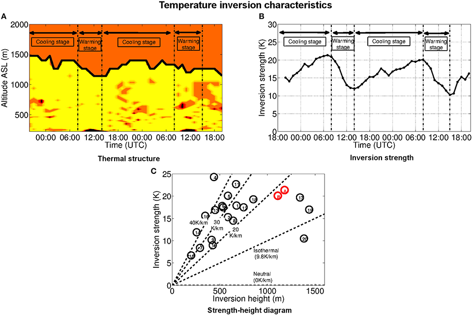
Figure 10. (A) Vertical profile of $\frac{\partial \theta }{\partial z}$ above point Gr (see Figure 7A) from 27 December, 18:00 UTC to 29 December, 20:00 UTC. Black : $\frac{\partial \theta }{\partial z}<0$. Orange : $0<\frac{\partial \theta }{\partial z}<|{\gamma }_{adiab}|$. Yellow : $\frac{\partial \theta }{\partial z}>|{\gamma }_{adiab}|$. (B) Inversion strength Δθ over the same time period. (C) Inversion strength vs. inversion height for 20 case studies of wintertime persistent inversions in the Rocky mountains (extracted and adapted from Whiteman et al., 1999b). Red symbols: parameters of the thermal inversion I₆ on 28 December 2006 (A) and 29 December (B).

The top of the inversion layer is underlined with a thick black line in Figure 10A. The inversion layer height little varies over the period, between 920 and 1255 m. The lowest values are observed during the warming stage, the inversion being slightly eroded both from the bottom by the shallow convective layer and from the top by warm subsidence (this erosion was classified as type II by Whiteman, 1982). The inversion then thickens during the cooling stage. In early afternoon, when the surface air temperature is the warmest, the inversion height is still of 920 m implying that the inversion is far from being destroyed.

The inversion strength Δθ, displayed in Figure 10B, varies between 10.3 and 21.3 K over the period. The cooling stage is associated with an intensification of the inversion strength, with a maximum value of about 21.3 K, while the lowest values are reached during the warming stage (equal to 12 K on 28 December and 10.3 K on 29 December, at 14:00 UTC). Thus, the inversion strength decreases by nearly 50% over a day but its smallest value is still equal to 10 K, attesting that the inversion is persistent and strong.

Computation of the heat deficit leads to huge values at sunrise, of 23.4 MJ m⁻² on 28 December and of 20.7 MJ m⁻² on 29 December while the values remain strong at sunset, comprised between 11.7 and 12.8 MJ m⁻² for these 2 days. These values are close to those inferred from the ground observations (see Figure 3). They are significantly higher than those estimated by Whiteman et al. (1999a) from inversion measurements in midsize Colorado valleys (1−8 MJ m⁻² at sunrise) but of the same order as the values computed for the most extreme inversions in three valleys of size comparable to that of the Grenoble valleys.

Whiteman et al. (1999a) indeed compared the characteristics of inversions observed in 20 valleys of the Rocky mountains, which are reproduced in Figure 10C. Each valley is referred to by a number in a (h_i, Δθ) diagram and the characteristics of the persistent inversion I₆ estimated on December 28–29 are superimposed. The heat deficit for a given valley is proportional to the area below the line joining the origin to the valley number, implying that the most intense inversions are found in the right upper corner of the diagram. These involve for instance the Bullfrog basin (number 17) located north-east of the Grand Canyon and inversion I₆. I₆ therefore ranges among the extreme inversions, which is consistent with this inversion to be the strongest of the winter of 2006–2007.

6. Summary and Conclusion

The purpose of this paper was to investigate the valley-scale circulation in the atmospheric boundary layer (ABL) of the Grenoble valleys, along with its thermodynamical structure, during persistent inversions of the 2006–2007 winter. Ground-based observations of temperature and high-resolution numerical simulations have been used for this analysis.

The first step was to detect persistent inversions from the 2-m air temperature data, a detailed analysis of which being reported in Largeron and Staquet (2016). A criterion was introduced for this purpose, based upon the temperature difference between the valley bottom and the valley top. This criterion was shown to be equivalently expressed in terms of the valley heat deficit inside the inversion layer, which represents the heat required to destroy the inversion layer. Similarly, Whiteman et al. (1999a,b) used such criterion to identify persistent cold-air pools in the Salt Lake valley. Nine episodes were detected from November to February, which all coincide with the nine strongest PM₁₀ air-pollution episodes of that winter. These wintertime persistent inversions have a cumulated duration of one third of the total winter duration; they occur during anticyclonic conditions and are triggered by a mid-level advection of a warm air mass, as shown in Largeron and Staquet (2016). The simple method proposed here may serve as a reliable technique to detect persistent inversions from ground-based temperature data when no radio-soundings are available.

Numerical simulations were next performed with the MesoNH-SURFEX coupled model to analyse the persistent inversions, from formation to destruction. Only the stagnation stage, during which the inversion does not evolve from one day to the next, corresponding to the heart of an episode, is reported in the present paper. Several sensitivity and validation tests were performed to assess the validity of the computations, among which the sensitivity to the vertical resolution was investigated. It was found that a vertical resolution of 15 m at the ground allows the gross features of the atmospheric boundary-layer circulation to be reproduced, a resolution of at least 4 m at the ground being required for quantitative comparison with the 2-m air temperature to be obtained at the bottom of the valley. With a vertical resolution coarser than 15 m, the inversion layer is poorly represented, with a too weak strength due to a hot bias at the bottom of the valley and a cold bias at the valley top. This can be explained by the need to correctly represent the down-slope winds which drive and maintain the inversion layer in inducing cold-air drainage along the slopes, from the valley top down to the valley bottom.

Numerical simulations were thus performed in two steps. Firstly, among the nine persistent inversions, the five longest and strongest inversions, which exhibit a stagnation stage, were simulated as case studies, over a 10-h night with a vertical resolution of 15 m close to the ground. Focusing again upon one night in the heart of each episode, the main conclusions are that: (i) an inversion layer has formed up to an altitude of about 1500 m, whose absolute temperature gradient is nearly constant and of about 10 K km⁻¹. (ii) whatever the persistent inversion episode, the atmosphere can be decomposed into three layers : the free troposphere above 3000 m ASL, a buffer zone between 1500 and 3000 m ASL in which the large-scale synoptic wind is orographically channelled, and the inversion layer below 1500 m ASL. The inversion layer is decoupled from the atmosphere above whatever the episode, thereby recovering a common feature of wintertime persistent inversions. As a result, the atmospheric circulation in this inversion layer is controlled by thermal winds created by the nocturnal cooling of the ground; (iii) a local dynamics set in in the inversion layer, which is independent of the episode. These dynamics are characterized by a vertical layering resulting from the superposition of four main valley winds flowing from the tributary valleys of the Grenoble basin.

It follows that a detailed account of the heart of a persistent episode can be obtained by performing a high-resolution simulation of any of the five episodes. This is the second step of the numerical study. Two days during the heart of the longest and most extreme inversion were thus simulated with a 4-m vertical resolution close to the ground. The horizontal wind field appears to have a quasi-deterministic structure, with a veering shear with altitude, the wind speed and direction at a given altitude being controlled by a down-valley wind. Large-scale vortex structures appear at the entrance of the Grésivaudan valley and along the flank of the Belledonne range. A first guess of the impact of this circulation on air quality was addressed by computing the stagnation and recirculation indices introduced by Allwine and Whiteman (1994). Stagnation regions critical for air quality were thus identified, especially south to the agglomeration and along the flank of the Belledonne range where wind speeds remain low and vortices form.

A detailed account of the diurnal evolution of the thermal inversion was also obtained: the height of the inversion varies between about 900 and 1200 m, the lowest value occurring around 14:00 UTC when the inversion is eroded from below by a shallow convective layer of at most 50 m above the ground and from the top by a warm subsidence. The temperature difference between inversion top and bottom ranges between about 10 K (at 14:00 UTC) and 21 K (at 08:00 UTC). These features are those of a very strong and deep inversion and are actually similar to the most extreme inversions recorded by Whiteman et al. (1999a) in the Grand Canyon.

As already pointed out, no wintertime field campaign has ever been undertaken in the Grenoble valleys although this area is densely populated and strongly industrialized. Combined with the present results regarding stagnation of the atmospheric surface layer, this leads to severe human health issues. It would be very desirable to launch such a campaign, as the collected data would offer the possibility to get a better estimate of the validity of numerical simulations, regarding the quasi-deterministic pattern of the wind profiles or the thermal structure of the inversion layer we found. Field data would also allow us to get access to much finer scales than those analysed in this paper, such as surface fluxes, the knowledge of which is crucially needed to validate the ABL forcing of a surface-atmosphere coupled model or to improve the physical parameterizations. Obviously, complementary chemical and air quality studies would also benefit from acute knowledge of local fine-scale atmospheric dynamics.

Author Contributions

YL: Author of the research presented in the manuscript and of the original manuscript. CS: Contribute to the manuscript.

Conflict of Interest Statement

The authors declare that the research was conducted in the absence of any commercial or financial relationships that could be construed as a potential conflict of interest.

The reviewer VM declared a shared affiliation, though no other collaboration, with one of the authors YL to the handling Editor, who ensured that the process nevertheless met the standards of a fair and objective review.

Acknowledgments

The present work was supported by a funding from région Rhône-Alpes. Computations were carried out on the machines of the French computer center IDRIS.

Supplementary Material

The Supplementary Material for this article can be found online at: https://www.frontiersin.org/article/10.3389/feart.2016.00070

References

Air Rhône-Alpes (2011). Suivi des Polluants Réglementés Dans la Vallée de l'Arve. Technical report, Air Rhône-Alpes.

Allwine, K., and Whiteman, C. (1994). Single-station integral measures of atmospheric stagnation, recirculation and ventilation. Atmos. Environ. 28, 713–721. doi: 10.1016/1352-2310(94)90048-5

CrossRef Full Text | Google Scholar

Banta, R., Darby, L., Fast, J., Pinto, J., Whiteman, C., Shaw, W., et al. (2004). Nocturnal low-level jet in a mountain basin complex. Part I: evolution and effects on local flows. J. Appl. Meteorol. 43, 1348–1365. doi: 10.1175/JAM2142.1

CrossRef Full Text | Google Scholar

Chemel, C., Arduini, G., Staquet, C., Largeron, Y., Legain, D., Tzanos, D., et al. (2016). Valley heat deficit as a bulk measure of wintertime particulate air pollution in the Arve River Valley. Atmos. Environ. 128, 208–215. doi: 10.1016/j.atmosenv.2015.12.058

CrossRef Full Text | Google Scholar

Couach, O., Balin, I., Jiménez, R., Ristori, P., Perego, S., Kirchner, F., et al. (2003). An investigation of ozone and planetary boundary layer dynamics over the complex topography of Grenoble combining measurements and modeling. Atmos. Chem. Phys. Discuss. 3, 797–825. doi: 10.5194/acpd-3-797-2003

CrossRef Full Text | Google Scholar

Cuxart, J. (2015). When can a high-resolution simulation over complex terrain be called LES? Front. Earth Sci. 3:87. doi: 10.3389/feart.2015.00087

CrossRef Full Text | Google Scholar

Cuxart, J., Bougeault, P., and Redelsperger, J. (2000). A turbulence scheme allowing for mesoscale and large-eddy simulations. Q. J. R. Meteorol. Soc. 126, 1–30. doi: 10.1002/qj.49712656202

CrossRef Full Text | Google Scholar

Cuxart, J., Conangla, L., and Jiménez, M. (2015). Evaluation of the surface energy budget equation with experimental data and the ecmwf model in the ebro valley. J. Geophys. Res. Atmos 120, 1008–1022. doi: 10.1002/2014JD022296

CrossRef Full Text | Google Scholar

Cuxart, J., and Jiménez, M. (2007). Mixing processes in a nocturnal low-level jet: An les study. J. Atmos. Sci. 64, 1666–1679. doi: 10.1175/JAS3903.1

CrossRef Full Text | Google Scholar

Cuxart, J., Jiménez, M., and Martínez, D. (2007). Nocturnal meso-beta basin and katabatic flows on a midlatitude island. Month. Weather Rev. 135, 918. doi: 10.1175/MWR3329.1

CrossRef Full Text | Google Scholar

Drobinski, P., Steinacker, R., Richner, H., Baumann-Stanzer, K., Beffrey, G., Benech, B., et al. (2007). Föhn in the rhine valley during map: a review of its multiscale dynamics in complex valley geometry. Q. J. R. Meteorol. Soc. 133, 897–916. doi: 10.1002/qj.70

CrossRef Full Text | Google Scholar

Favez, O., El Haddad, I., Piot, C., Boréave, A., Abidi, E., Marchand, N., et al. (2010). Inter-comparison of source apportionment models for the estimation of wood burning aerosols during wintertime in an Alpine city (Grenoble, France). Atmos. Chem. Phys. Discuss 10, 559–613. doi: 10.5194/acpd-10-559-2010

CrossRef Full Text | Google Scholar

Fernando, H. (2010). Fluid dynamics of urban atmospheres in complex terrain. Annu. Rev. Fluid Mech. 42, 365–389. doi: 10.1146/annurev-fluid-121108-145459

CrossRef Full Text | Google Scholar

Flamant, C., Drobinski, P., Nance, L., Banta, R., Darby, L., Dusek, J., et al. (2002). Gap flow in an alpine valley during a shallow south föhn event: Observations, numerical simulations and hydraulic analogue. Q. J. R. Meteorol. Soc. 128, 1173–1210. doi: 10.1256/003590002320373256

CrossRef Full Text | Google Scholar

Foken, T. (2008). The energy balance closure problem: an overview. Ecol. Appl. 18, 1351–1367. doi: 10.1890/06-0922.1

PubMed Abstract | CrossRef Full Text | Google Scholar

Gohm, A., Harnisch, F., Vergeiner, J., Obleitner, F., Schnitzhofer, R., Hansel, A., et al. (2009). Air pollution transport in an Alpine valley: results from airborne and ground-based observations. Boundary-layer Meteorol. 131, 441–463. doi: 10.1007/s10546-009-9371-9

CrossRef Full Text | Google Scholar

Harnisch, F., Gohm, A., Fix, A., Schnitzhofer, R., Hansel, A., and Neininger, B. (2009). Spatial distribution of aerosols in the Inn Valley atmosphere during wintertime. Meteorol. Atmos. Phys. 103, 223–235. doi: 10.1007/s00703-008-0318-3

CrossRef Full Text | Google Scholar

Lafore, J., Stein, J., Asencio, N., Bougeault, P., Ducrocq, V., Duron, J., et al. (1998). The Meso-NH atmospheric simulation system. Part I: Adiabatic formulation and control simulations. Ann. Geophys. 16, 90–109. doi: 10.1007/s00585-997-0090-6

CrossRef Full Text | Google Scholar

Lareau, N., Crosman, E., Whiteman, C., Horel, J., Hoch, S., Brown, W., et al. (2013). The persistent cold-air pool study. Bull. Am. Meteorol. Soc. 94, 51–63. doi: 10.1175/BAMS-D-11-00255.1

CrossRef Full Text | Google Scholar

Largeron, Y. (2010). Dynamics of the Stable Atmospheric Boundary Layer over Complex Terrain. Application to PM10 Pollution Episodes in Alpine Valleys. Ph.d. thesis, Université de Grenoble.

Largeron, Y., and Staquet, C. (2016). Persistent inversion dynamics and wintertime PM₁₀ air pollution in Alpine valleys. Atmos. Environ. 135, 92–108. doi: 10.1016/j.atmosenv.2016.03.045

CrossRef Full Text | Google Scholar

Levy, I., Mahrer, Y., and Dayan, U. (2009). Coastal and synoptic recirculation affecting air pollutants dispersion: a numerical study. Atmos. Environ. 43, 1991–1999. doi: 10.1016/j.atmosenv.2009.01.017

CrossRef Full Text | Google Scholar

Lienhard, J., and van Atta, C. (1990). The decay of turbulence in thermally stratified flows. JFM 210, 57–112. doi: 10.1017/S0022112090001227

CrossRef Full Text | Google Scholar

Mahrt, L. (2014). Stably stratified atmospheric boundary layers. Annu. Rev. Fluid Mech. 46, 23–45. doi: 10.1146/annurev-fluid-010313-141354

CrossRef Full Text | Google Scholar

Martínez, D., Jiménez, M., Cuxart, J., and Mahrt, L. (2010). Heterogeneous nocturnal cooling in a large basin under very stable conditions. Boundary-layer Meteorol. 137, 97–113. doi: 10.1007/s10546-010-9522-z

CrossRef Full Text | Google Scholar

Masson, V. (2000). A physically-based scheme for the urban energy budget in atmospheric models. Bound. Layer Meteor. 94, 357–397. doi: 10.1023/A:1002463829265

CrossRef Full Text | Google Scholar

Masson, V., Champeaux, J., Chauvin, F., Meriguet, C., and Lacaze, R. (2003). A global data base of land surface parameters at 1 km resolution in meteorological and climate model. J. Appl. Meteor. Climatol. 16, 1261–1282. doi: 10.1175/1520-0442-16.9.1261

CrossRef Full Text | Google Scholar

Masson, V., Le Moigne, P., Martin, E., Faroux, S., Alias, A., Alkama, R., et al. (2013). The surfexv7.2 land and ocean surface platform for coupled or offline simulation of earth surface variables and fluxes. Geosci. Model Dev. 6, 929–960. doi: 10.5194/gmd-6-929-2013

CrossRef Full Text | Google Scholar

Neff, W., and King, C. (1989). The accumulation and pooling of drainage flows in a large basin. J. Appl. Meteor. 28, 518–529.

Google Scholar

Noilhan, J., and Planton, S. (1989). A simple parameterization of land surface processes for meteorological models. Month. Weather Rev. 117, 536.

Google Scholar

Pope, C. A., Burnett, R. T., Thun, M. J., Calle, E. E., Krewski, D., Ito, K., et al. (2002). Lung cancer, cardiopulmonary mortality, and long-term exposure to fine particulate air pollution. JAMA 287, 1132–1141. doi: 10.1001/jama.287.9.1132

PubMed Abstract | CrossRef Full Text | Google Scholar

Price, J., Vosper, S., Brown, A., Ross, A., Clark, P., Davies, F., et al. (2011). COLPEX: field and numerical studies over a region of small hills. Bull. Am. Meteorol. Soc. 92, 1636–1650. doi: 10.1175/2011BAMS3032.1

CrossRef Full Text | Google Scholar

Reeves, H. D., and Stensrud, D. J. (2009). Synoptic-scale flow and valley cold pool evolution in the western united states. Weather Forecast. 24, 1625–1643. doi: 10.1175/2009WAF2222234.1

CrossRef Full Text | Google Scholar

Schnitzhofer, R., Norman, M., Dunkl, J., Wisthaler, A., Gohm, A., Obleitner, F., et al. (2007). Vertical distribution of air pollutants in the Inn Valley atmosphere in winter 2006. Geophys. Res. Abstr.

Google Scholar

Silcox, G. D., Kelly, K. E., Crosman, E. T., Whiteman, C. D., and Allen, B. L. (2012). Wintertime PM 2.5 concentrations during persistent, multi-day cold-air pools in a mountain valley. Atmos. Environ. 46, 17–24.

Google Scholar

Stull, R. (1988). An Introduction to Boundary Layer Meteorology. Kluwer.

Google Scholar

Sun, J., Nappo, C., Mahrt, L., Belusic, D., Grisogono, B., Stauffer, D., et al. (2015). Review of wave-turbulence interactions in the stable atmospheric boundary layer. Rev. Geophys. 53, 956–993. doi: 10.1002/2015RG000487

CrossRef Full Text | Google Scholar

Venegas, L., and Mazzeo, N. (1999). Atmospheric stagnation, recirculation and ventilation potential of several sites in Argentina. Atmos. Res. 52, 43–57. doi: 10.1016/S0169-8095(99)00030-7

CrossRef Full Text | Google Scholar

Vosper, S., Hugues, J., Lock, A., Sheridan, P., Ross, A., Jemmett-Smith, A., et al. (2014). Cold-pool formation in a narrow valley. Q. J. R. Meteorol. 140, 699–714. doi: 10.1002/qj.2160

CrossRef Full Text | Google Scholar

Wei, L., Pu, Z., and Wang, S. (2013). Numerical simulation of the life cycle of a persistent wintertime inversion over salt lake city. Bound. Layer Meteor. 148, 399–418. doi: 10.1007/s10546-013-9821-2

CrossRef Full Text | Google Scholar

Whiteman, C. (1982). Breakup of temperature inversions in deep mountain valleys: Part I. observations. J. Appl. Meteorol. 21, 270–289.

Google Scholar

Whiteman, C. (2000). Mountain Meteorology: Fundamentals and Applications. Oxford University Press, USA.

Google Scholar

Whiteman, C., Bian, X., and Zhong, S. (1999a). Wintertime evolution of the temperature inversion in the Colorado Plateau Basin. J. Appl. Meteorol. 38, 1103–1117.

Google Scholar

Whiteman, C., and Doran, J. (1993). The relationship between overlying synoptic-scale flows and winds within a valley. J. Appl. Meteorol. 32, 1669–1682.

Google Scholar

Whiteman, C., Muschinski, A., Zhong, S., Fritts, D., Hoch, S., Hahnenberger, M., et al. (2008). Metcrax 2006. Bull. Am. Met. Soc. 89, 1665–1680. doi: 10.1175/2008bams2574.1

PubMed Abstract | CrossRef Full Text | Google Scholar

Whiteman, C., Zhong, S., and Bian, X. (1999b). Wintertime boundary layer structure in the Grand Canyon. J. Appl. Meteorol. 38, 1084–1102.

Google Scholar

Whiteman, C., Zhong, S., Shaw, W., Hubbe, J., Bian, X., and Mittelstadt, J. (2001). Cold pools in the Columbia Basin. Weather Forecast. 16, 432–447. doi: 10.1175/1520-0434(2001)016<0432:CPITCB>2.0.CO;2

CrossRef Full Text | Google Scholar

Whiteman, C. D., Eisenbach, S., Pospichal, B., and Steinacker, R. (2004). Comparison of vertical soundings and sidewall air temperature measurements in a small alpine basin. J. Appl. Meteorol. 43, 1635–1647. doi: 10.1175/JAM2168.1

CrossRef Full Text | Google Scholar

Wolyn, P., and McKee, T. (1989). Deep stable layers in the intermountain western united states. Mon. Wea. Rev. 117, 461–472.

Google Scholar

Zhong, S., Whiteman, C., Bian, X., Shaw, W., and Hubbe, J. (2001). Meteorological processes affecting the evolution of a wintertime cold air pool in the Columbia basin. Month. Weather Rev. 129, 2600–2613. doi: 10.1175/1520-0493(2001)129<2600:MPATEO>2.0.CO;2

CrossRef Full Text | Google Scholar

Zhou, B., and Chow, F. (2013). Nighttime turbulent events in a steep valley: a nested large-eddy simulation study. J. Atmos. Sci. 70, 3262–3276. doi: 10.1175/JAS-D-13-02.1

CrossRef Full Text | Google Scholar