Stikine Icefield Mass Loss between 2000 and 2013/2014

1. Introduction

The glaciers of Alaska and northwest Canada provide a disproportionately larger contribution to global sea level rise (SLR) than is expected, based on their surface area. The glaciers are amongst the largest contributors to SLR after the Greenland and Antarctica ice sheets (e.g., Gardner et al., 2013). Exactly how this glacier mass loss in this region has been partitioned between land-, lacustrine-, and tidewater terminating glaciers has only recently been determined —Larsen et al. (2015) find that between 1994 and 2013, the fast-moving tidewater glaciers contribute only 6% of the total mass loss of the region. Using a different method, McNabb et al. (2014) estimated that 27 marine-terminating glaciers (representing 96% of the tidewater glacier area in Alaska) accounted for 20% of mass loss between 2004 and 2010. Larsen et al. (2015) also find significant glacier-to-glacier variations in the rate of mass loss. These glacier-to-glacier variations are important because Larsen et al. (2015) rely on extrapolation from their observation of 116 glaciers, representing 41% of the glaciated area, to the entire region.

To better understand the regional variations in the partitioning of mass loss between glaciers of different terminus types, we have made a detailed study of nearly the entire glaciated area of the Stikine Icefield—consisting of 5800 km² of ice cover in the Coast Mountains (e.g., Burgess et al., 2013) on the US-Canada border. The Stikine Icefield is the furthest south of the major northern hemisphere icefields (Figure 1). We focus on this area because it has not received recent detailed study unlike the nearby regions (Figure 1) of Glacier Bay (e.g., Johnson et al., 2013) and the Juneau Icefield (e.g., Melkonian et al., 2014) and our study builds upon the coverage of Larsen et al. (2015) that surveyed about one quarter of the icefield.

FIGURE 1

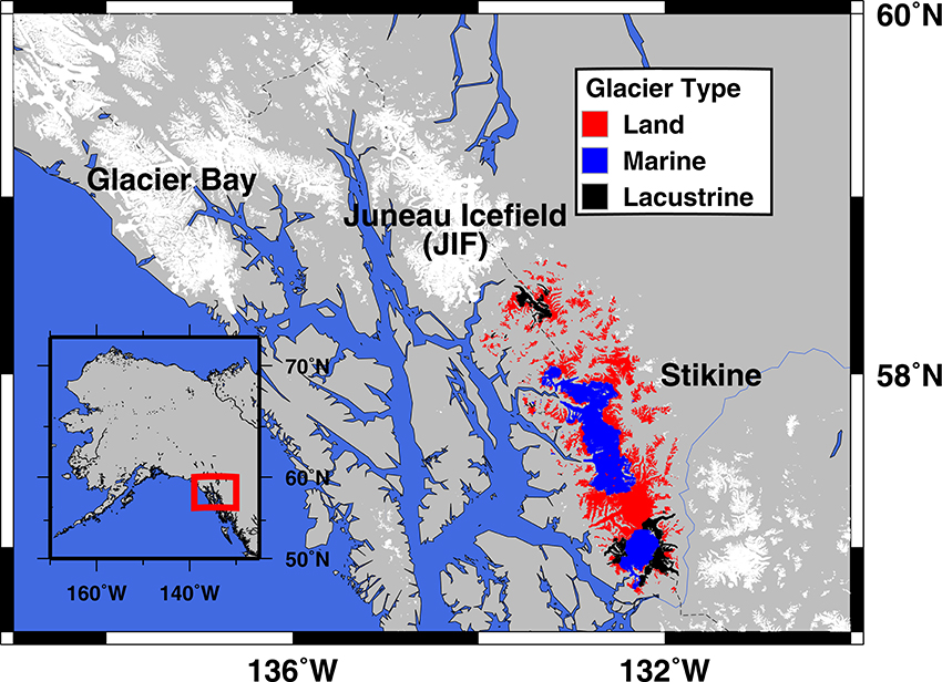
Figure 1. Glaciers of southeast Alaska. Study area consists of Stikine Icefield glaciers where terminus type is color-coded (red for land-terminating, blue for marine and green for lacustrine) and covers approximately 5800 km².

Previous studies investigating mass loss (e.g., Larsen et al., 2007; Berthier et al., 2010; Arendt et al., 2013; Larsen et al., 2015) and glacier dynamics (e.g., O'Neel et al., 2001, 2003; McNabb et al., 2014) at Alaskan glaciers cover the Stikine Icefield, which is a small fraction of these generally regional studies. These studies lack the resolution to discern individual glaciers (e.g., Arendt et al., 2013), have incomplete coverage (e.g., Larsen et al., 2015), or do not incorporate the most recent data (e.g., Larsen et al., 2007; Berthier et al., 2010). We update mass loss estimates for the Stikine Icefield by calculating thinning rates ($\frac{dh}{dt}$) between 2000 and 2013/2014, applying a weighted linear regression to stacked digital elevation models (DEMs) derived from satellite stereo-optical data and compare these results with airborne LIDAR centerline elevation tracks.

We also measure glacier velocities using feature tracking on optical satellite imagery acquired between 1985 and 2014, looking for inter-annual speed changes. Using selected velocity maps, along with estimates of glacier thickness, we constrain the frontal ablation flux (including calving and submarine melt) at the four largest marine-terminating glaciers on the Stikine Icefield: North Sawyer, South Sawyer, Dawes and LeConte glaciers. Together, these four glaciers account for 90–95% of the total ice area drained by marine-terminating glaciers on the Stikine Icefield.

There are two overarching methods through which Alaskan glaciers contribute to sea level rise—surface melt, with meltwater subsequently reaching the ocean, and ice moving from land into the marine environment via frontal ablation. Ablation at land-terminating glaciers is dominated by the former (e.g., Larsen et al., 2015). Frontal ablation, the sum of calving and submarine melting, is sometimes the dominant means of mass loss at marine-terminating glaciers (e.g., Burgess et al., 2013; McNabb et al., 2014), where ice speeds can be relatively high. We examine whether mass loss due to frontal ablation is a substantial fraction of the total mass loss from the Stikine Icefield by comparing $\frac{dh}{dt}$ by elevation for marine- vs. land-terminating glaciers.

2. Data and Methods

Figure S1 provides a summary of the elevation data used in this study. Thinning rates, or $\frac{dh}{dt}$, are estimated by applying a weighted linear regression on a pixel-by-pixel basis to 53 ASTER DEMs from 2000 to 2014 stacked with the Shuttle Radar Topography Mission (SRTM) DEM (e.g., Farr et al., 2007), acquired in February of 2000. The SRTM DEM off-ice elevations serve as the reference surface to which we horizontally and vertically coregister the ASTER DEMs using the “pc_align” program from the Ames Stereo Pipeline toolset (Broxton and Edwards, 2008; Moratto et al., 2013) that uses the Iterative Closest Point (ICP) algorithm (see Section 5.2.5 of the Ames Stereo Pipeline manual). The SRTM is a radar product that is not substantially affected by typical sources of error that cause erroneous ASTER elevations, such as cloud or snow cover, so we use it to filter out bad elevations in the ASTER DEMs by limiting their deviation from the SRTM elevation at each pixel. All SRTM elevations above the regional ELA of approximately 1000 m (e.g., Larsen et al., 2007) are adjusted 2 m upwards to account for C-band penetration based on a comparison of C- and X-band elevations from SRTM (Figure S8), although further work is needed to see if this under-estimates the penetration in Alaska (Berthier et al., 2016). We summarize the magnitude of these error sources in Table S2—the combined uncertainty is about 33% of the total mass loss.

ASTER acquires stereo-imagery in the same wavelength band using independent nadir- and backward-looking telescope assemblies (bands 3N and 3B, respectively, e.g., Fujisada et al., 2005). The Land Processes Distributed Active Archive Center (LP DAAC) uses this stereo-imagery to produce an on-demand DEM for each ASTER acquisition requested (e.g., Fujisada et al., 2005). Full details of the methodology for the feature tracking and $\frac{dh}{dt}$ processing are given in Willis et al. (2012a), Melkonian et al. (2013), and Melkonian et al. (2014), as well as in the Supplementary Material.

The uncertainty on ASTER DEMs can be relatively high (e.g., Fujisada et al., 2005), the average uncertainty of the 53 DEMs we incorporate into our $\frac{dh}{dt}$ is ± 19 m. We validate the ASTER/SRTM $\frac{dh}{dt}$, which have an average last date of 2013/09/05, by comparing the rates from DEM-differencing between four WorldView DEMs from 2013 and the SRTM DEM to the ASTER $\frac{dh}{dt}$ over the same areas (which correspond to ~14% of the total glaciated area). Although the noise on individual ASTER DEMs is large, the time series approach using dozens of dates spread over different seasons overcomes some of the issues of differencing only two DEMs, without applying seasonal corrections (e.g., Willis et al., 2012b; Wang and Kääb, 2015; Berthier et al., 2016). The WorldView DEMs are coregistered to the SRTM DEM using the same method applied to the ASTER DEMs.

We also apply DEM-differencing to LIDAR elevation data from 2013 and the SRTM DEM from 2000 to produce 2000–2013 LIDAR/SRTM $\frac{dh}{dt}$. Mass loss for the entire ice area on the Stikine Icefield drained by marine-terminating glaciers is extrapolated based on hypsometry from 2000 to 2013 LIDAR/SRTM $\frac{dh}{dt}$ for LeConte Glacier, the only marine-terminating glacier on the Stikine Icefield included in Larsen et al. (2015). We do this in order to determine whether the $\frac{dh}{dt}$ we calculate for the other marine-terminating glaciers on the Stikine Icefield add to our understanding of mass loss there beyond the results of Larsen et al. (2015). The LIDAR/SRTM rates are also used as further validation of the ASTER $\frac{dh}{dt}$.

Ice velocities are measured by applying normalized cross-correlation, or “feature tracking,” to suitable image pairs using the “ampcor” tool from the Repeat Orbit Interferometry PACkage (ROI_PAC Rosen et al., 2004). Our feature tracking data are 223 pairs of orthorectified optical imagery acquired by Landsat 5, 7, and 8 between 1985 and 2014 (Figure S2), as well as one pair of WorldView images from June 2008. The WorldView images are orthorectified to the closest DEM in time, which is one of the four WorldView DEMs from 2013/06/18. We apply post-processing that removes a ramp calculated from the velocity results over off-ice areas, filters out incoherent noise, and mitigates orthorectification errors by removing a linear trend between off-ice velocities and elevations from a DEM (e.g., as suggested in Ahn and Howat, 2011). Our analysis complements the existing work of McNabb et al. (2014) who also used Landsat pairs to calculate velocities, by using an independent method and a slightly different set of data. As noted by McNabb et al. (2014), there are not enough images at each glacier to determine the seasonal velocity variation, but in aggregate, it is clear that there is a seasonal variation in velocity (maximum in the March-May, their Figure 6) and so whenever we make statements about inter-annual velocity variations, we compare similar seasons.

We want to determine whether the total frontal ablation flux is large enough to accommodate the higher average 2000 to 2013/2014 mass loss at marine- vs. land-terminating glaciers. Frontal ablation flux is estimated from our glacier velocities along front transects on the four largest marine-terminating glaciers on the Stikine Icefield at 60 m intervals (which cover roughly 90–95% of the total marine-terminating glacier area—North Sawyer, South Sawyer, Dawes and LeConte glaciers, speed profiles shown in Figure S3). We assume that the depth-averaged velocity is the same as the surface velocity (e.g., Burgess et al., 2013). The lower bound on the depth-averaged velocity is set to 80% of the surface velocity (Cuffey and Paterson, 2010; Burgess et al., 2013), so the lower bound flux estimates are 80% of our best estimates. The fact that we only use spring velocities may bias our flux estimates too high by 6%, as determined by an average frontal ablation rate in a regional study of 27 Alaskan tidewater glaciers by McNabb et al. (2014).

Thicknesses are obtained using surface elevations and a maximum depth from fjord bathymetry from the USGS by assuming either a trapezoidal or triangular cross-section, whichever is most appropriate given the available evidence. To estimate the cross-section, we first set the thickness to zero at the surface elevation for the first and last points on the transect. We assume the thickness goes linearly to the surface elevation plus the maximum depth at the middle point for the triangular cross-section, and to the surface elevation plus the maximum depth for the middle half of the transect in the case of the trapezoidal cross-section (Figure S4). The approximate shape of the cross-sections at the glacier fronts for North and South Sawyer glaciers are determined by comparing ice elevations along the front transects in 2000 from the SRTM DEM to ice elevations in 2013 from the WorldView DEMs (Figure S5). The cross-section at the front transect of LeConte Glacier is assumed to be triangular based on the cross-section shown in Figure 2A of O'Neel et al. (2003), and the cross-section of Dawes Glacier is assumed to be trapezoidal based on the bathymetry data available from the USGS.

The magnitude of the surface velocity perpendicular to the transect multiplied by the cross-sectional area (the interval width multiplied by the thickness) gives the flux for each interval, and summing together the flux for all intervals yields a total flux across the transect. This assumes that ice flux is approximately equal to the frontal ablation flux (i.e., that instantaneous changes in the glacier length are small). We produce a total uncertainty on the flux estimates by estimating and combining the uncertainties on the velocities, surface elevations, $\frac{dh}{dt}$ and depths. We calculate uncertainty due to the velocities similarly to the way we calculate flux. Instead of multiplying the speed by the cross-sectional area, we multiply the uncertainty by the cross-sectional area, and we account for the independence of the velocity measurements by dividing by the width of the reference window used during feature tracking. The uncertainty on the surface elevations is the uncertainty of the DEM used to provide the elevations, which is set to 5 m for the SRTM DEM and applied uniformly to the entire transect. The uncertainty of the WorldView DEMs is set to the standard deviation of the off-ice elevation differences between the WorldView DEM and the SRTM DEM (± 12–13 m). The uncertainty on the ASTER/SRTM $\frac{dh}{dt}$ is described in detail in the supplemental material. The WorldView/SRTM $\frac{dh}{dt}$ uncertainties are obtained by adding the individual DEM uncertainties in quadrature. The uncertainty on the maximum depth is estimated from the variability of USGS bathymetry measurements within the deepest contour, and this value is 40 m for North Sawyer, 50 m for South Sawyer, 60 m for Dawes, and 30 m for LeConte. These uncertainties are added in quadrature to produce an overall uncertainty for the flux estimates. Further details of the frontal ablation flux are in the Supplementary Material.

3. Results

Figure 2 shows a map of the $\frac{dh}{dt}$ calculated from the SRTM and ASTER DEMs between 2000 and 2013/2014. The maximum thinning rates are at low elevations of glaciers with all terminus types (Figure 3), but with the maximum values on the western, marine side. The highest $\frac{dh}{dt}$ of around −17–19 m w.e. yr⁻¹ occur at the fronts of the marine-terminating South and North Sawyer glaciers. The mass loss rate between 2000 and 2013/2014 at the Stikine Icefield from the SRTM and ASTER DEMs is −3.3 ± 1.1 Gt yr⁻¹, equivalent to an area-averaged elevation change rate of −0.57 ± 0.18 m w.e. yr⁻¹. Marine-terminating glaciers are thinning at an average rate of −0.78 ± 0.17 m w.e. yr⁻¹ (−1.5 ± 0.3 Gt yr⁻¹), which is faster than the average elevation change rate of -0.34 ± 0.17 m w.e. yr⁻¹ at land-terminating glaciers (−0.9 ± 0.4 Gt yr⁻¹).

FIGURE 2

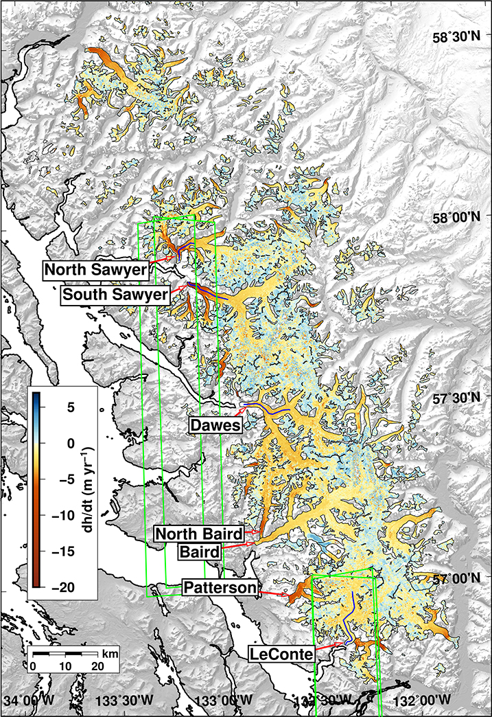
Figure 2. Map of $\frac{dh}{dt}$ between 2000 and 2013/2014 for the Stikine Icefield from stacked ASTER DEMs and the SRTM DEM. The black lines indicate glacier boundaries (circa 2000). The purple lines at North Sawyer, South Sawyer, Dawes and LeConte glaciers indicate the locations of the centerline speed profiles shown in Figure 4. The green lines indicate the coverage of the four WorldView DEMs used in this study.

FIGURE 3

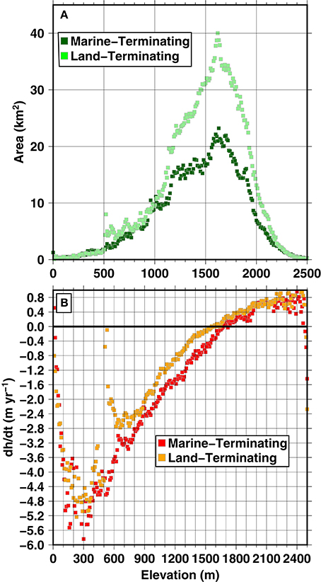
Figure 3. Hypsometry (A) and $\frac{dh}{dt}$ by elevation (B) for marine- and land-terminating glaciers on the Stikine Icefield using $\frac{dh}{dt}$ between 2000 and 2013/2014 calculated from stacked ASTER DEMs and the SRTM DEM. Note that the minimum $\frac{dh}{dt}$ is not always at the lowest elevation, both because the $\frac{dh}{dt}$ becomes zero in areas of retreat as well as the fact that there are few data points at low elevation (A).

The 2000–2013/2014 ASTER/SRTM $\frac{dh}{dt}$ match well with $\frac{dh}{dt}$ from DEM-differencing applied to four WorldView DEMs from 2013 and the SRTM DEM (Figure S6). We also compare the 2000–2013/2014 ASTER/SRTM $\frac{dh}{dt}$ over the area of the LIDAR centerline tracks from 2013 at LeConte, South Sawyer, North Sawyer and Dawes glaciers to see if the ASTER results match the more precise 2000–2013 LIDAR/SRTM $\frac{dh}{dt}$. The ASTER and LIDAR rates match within the average uncertainty of the ASTER $\frac{dh}{dt}$ (Figure S10) and show the same trends with elevation (Figure S9).

Figure 4 shows velocities along centerline longitudinal profiles for North Sawyer, Dawes, South Sawyer and LeConte glaciers (profile locations indicated in Figure 2). The four largest marine-terminating glaciers maintain near-front velocities between 1985 and 2014 that are significantly higher than the rest of the glaciers on the Stikine Icefield. All four glaciers retreat between one and two kilometers between 1984 and 2014 (Figure 5), but the terminus of LeConte Glacier has remained stable since 1999, whereas Dawes, South Sawyer and North Sawyer glaciers have receded since then (e.g., McNabb and Hock, 2014).

FIGURE 4

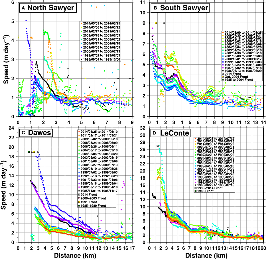
Figure 4. Centerline profiles of speeds between 1985 and 2014 for selected pairs at North Sawyer (A), South Sawyer (B), Dawes (C), and LeConte (D) glaciers. Front positions (determined from Landsat imagery) at selected dates indicated by squares.

FIGURE 5

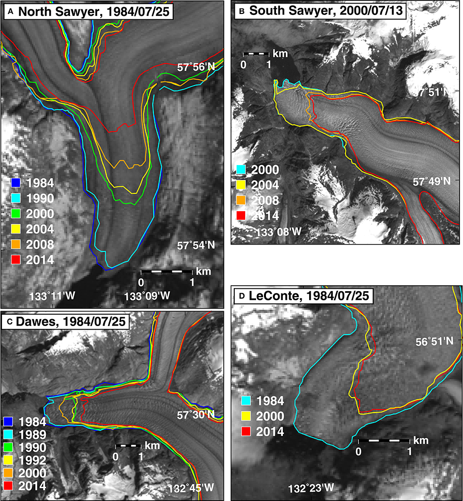
Figure 5. Selected front positions between 1984 and 2014 for the four major marine-terminating glaciers on the Stikine Icefield. Panels (A–D) show North Sawyer, South Sawyer, Dawes, and LeConte, respectively. The date of the Landsat background image is given in the panel label. “Cooler” colors are earlier front positions, “warmer” colors are more recent front positions.

The retreat at LeConte Glacier between 1985 and 1999 coincides with front acceleration from approximately 14 m day⁻¹ in summer 1986 to over 25 m day⁻¹ in spring 2003. Front velocities subsequently dropped to around 18–20 m day⁻¹ by spring/summer 2014 (Figure 4D).

Front velocities at South Sawyer glacier reached a maximum of 8 to 9 m day⁻¹ in July 1987 and then dropped to around 5 to 6 m day⁻¹ by July 1999 (Figure 4B). The front seems to have accelerated to 7 m day⁻¹ in the springs of 2003 and 2004 compared to the same season in 2002, associated with the substantial retreat of the front around a “bend” in the glacier during 2004. The terminus has continued to retreat since 2004 with a maximum velocity of 5 to 6 m day⁻¹ – still higher than the velocities from the same location (2–3 km from the 1985 front) and seasons prior to 2002.

The maximum front velocity at Dawes Glacier was steady at around 13 m day⁻¹ between 1985 and 1989 given the limited observations, during which time there was little change in the front position (Figure 4C). The maximum velocity increased to 18 m day⁻¹ during the summer and retreated by almost a kilometer between 1989 and 1991. By 1999–2000, the front's summer speed slowed to around 7 m day⁻¹ and the terminus advanced about 200 m. Retreat restarted as deceleration continued, and by 2014 the front had receded by a kilometer from its 1999 position and the maximum velocity during late spring dropped to 5 m day⁻¹.

Using velocities in May and June of 2014 for South Sawyer, North Sawyer, Dawes and LeConte glaciers, we estimate a combined 2014 frontal ablation flux of 1.18 ± 0.14 Gt yr⁻¹, equivalent to an area-averaged elevation change rate of 0.20 ± 0.02 m w.e. yr⁻¹ over the entire area of the Stikine Icefield. Figure 6 shows maps of velocities for each of the four glaciers, along with the transect used to calculate flux at each glacier. Table 1 shows best-guess and lower-bound fluxes for selected velocity pairs at the four glaciers, as well as the associated uncertainties.

FIGURE 6

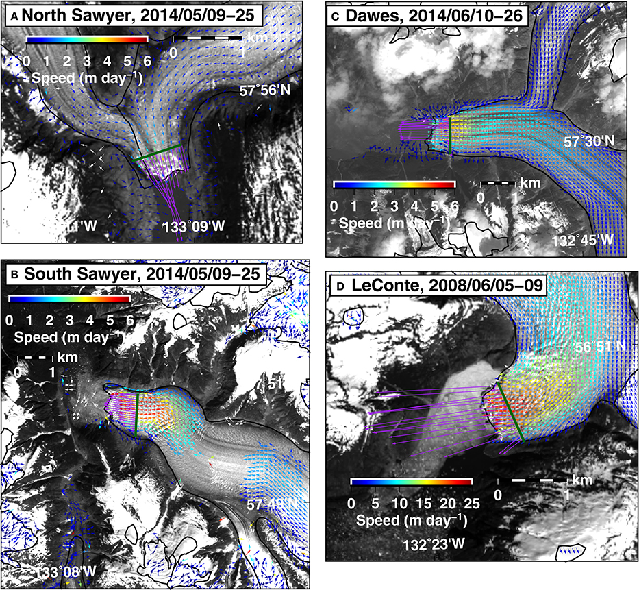
Figure 6. Map of velocities at North Sawyer, South Sawyer, Dawes, and LeConte glaciers from selected pairs (A–D). Dark green lines indicate transects used to calculate flux from the mapped velocities. Purple arrows highlight the velocities at each transect. Black lines indicate glacier boundaries.

TABLE 1

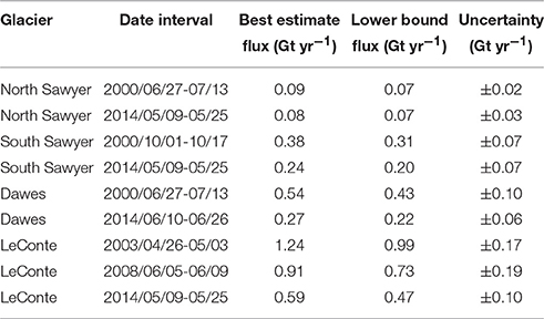
Table 1. Frontal ablation flux estimates for North Sawyer, South Sawyer, Dawes and LeConte glaciers from selected velocity pairs between 2000 and 2014.

The frontal ablation flux of LeConte Glacier decreases from 1.24 ± 0.17 Gt yr⁻¹ in spring 2003, to 0.91 ± 0.19 Gt yr⁻¹ in June 2008, to 0.59 ± 0.10 Gt yr⁻¹ in May 2014. The decrease is largely due to the average velocity along the transect decelerating from around 15 m day⁻¹ in 2003 and 2008 to about 9 m day⁻¹ in 2014. Frontal ablation flux at Dawes Glacier in summer 2000 is 0.54 ± 0.10 Gt yr⁻¹, decreasing to 0.27 ± 0.06 Gt yr⁻¹ in June 2014 along the same transect. Lower flux in 2014 is due a 25% drop in the average front speed and an average of 40 m of thinning along the transect since 2000. The frontal ablation flux of South Sawyer Glacier decreases from 0.38 ± 0.07 Gt yr⁻¹ in October of 2000 to 0.24 ± 0.07 Gt yr⁻¹ in May of 2014 along the same transect. The decrease is entirely the result of average thinning of more than 100 m along the front transect between 2000 and 2014, as the average terminus speed is higher in 2014 than 2000 (3.5 vs. 1.8 m day⁻¹, respectively) due to front retreat. Frontal ablation flux at North Sawyer Glacier is 0.09 ± 0.02 Gt yr⁻¹ in summer of 2000 and 0.08 ± 0.03 Gt yr⁻¹ in May of 2014 along the same transect. The average front speed along the transect accelerated from 0.7 m day⁻¹ in 2000 to 2.5 m day⁻¹ in 2014 as the front receded and approached the transect location, but the positive affect on flux was offset by average thinning of about 100 m along the transect.

4. Discussion

4.1. Thinning at Marine vs. Land-Terminating Glaciers

Marine-terminating glaciers are thinning more rapidly than land-terminating glaciers (-0.78 ± 0.17 m w.e. yr⁻¹ vs. -0.34 ± 0.17 m w.e. yr⁻¹, respectively)—could this be caused by marine-terminating glaciers having a larger concentration of area at lower elevations than land-terminating glaciers? Figure 3 shows that marine-terminating glaciers on the Stikine Icefield have more pronounced average thinning between elevations of around 100–2000 m than land-terminating glaciers, but a similar hypsometry. The land-terminating $\frac{dh}{dt}$ are consistently of lower magnitude than the marine-terminating $\frac{dh}{dt}$ at all elevations, but especially at lower elevations (<1600 m), leading to a clear and consistent difference between land- and marine- terminating average $\frac{dh}{dt}$ when summed over all elevations. Since we expect average thinning by elevation to be the approximately the same for land- and marine-terminating glaciers [all else being equal for this “climatic” component due to melt and precipitation (e.g., as proposed for Novaya Zemyla in the Russian Arctic, Moholdt et al., 2012)], the higher thinning at marine-terminating glaciers suggests a dynamic component to thinning, even though some of the marine-terminating glaciers have slowed down in recent decades. On the other hand, it is possible that all things are not equal in terms of the precipitation/melt change in the land- vs. marine terminating glaciers. But at the moment, there is no evidence that there are any systematic differences in hypsometry (Figure 3) or location of the two types of glaciers (Figure 1) that would suggest a bias in melt/preciptation at one terminus type vs. the other.

To further reinforce the difference between the marine- and land-terminating mass loss, we can extrapolate the results from one terminus type over the surface area of the other at each elevation. Multiplying the average marine-terminating glacier $\frac{dh}{dt}$ by the land-terminating area for each elevation bin yields a mass loss rate of −2.0 Gt yr⁻¹, vs. the observed value of −0.9 Gt yr⁻¹ over the same area using the land-terminating $\frac{dh}{dt}$. Conversely, multiplying the average land-terminating glacier $\frac{dh}{dt}$ by the marine-terminating glacier area for each elevation bin reduces the mass loss rate for the marine-terminating glacier area from the observed -1.5 Gt yr⁻¹ to −0.8 Gt yr⁻¹. Some factor or factors other than hypsometry must therefore be causing this “excess” thinning at marine-terminating glaciers on the Stikine Icefield, and one possible explanation is frontal ablation and drawdown.

In fact, the relatively high magnitude and distinct pattern of front velocities at the four largest marine-terminating glaciers suggest that dynamic thinning may account for at least part of the difference. The total frontal ablation flux from these four glaciers is high enough at both the beginning and end of the 2000 to 2013/2014 $\frac{dh}{dt}$ period to accommodate the estimated additional −0.7 Gt yr⁻¹ mass loss from marine-terminating glaciers above what it would be if they had the same $\frac{dh}{dt}$ by elevation as land-terminating glaciers (−0.8 Gt yr⁻¹ as calculated in the last paragraph).

The disproportionately high mass loss from marine-terminating glaciers is in stark contrast with mass loss from the adjacent Juneau Icefield to the north (e.g., Melkonian et al., 2014) where the flux from marine-terminating glaciers is essentially zero. This is in part because the only “marine-terminating” glacier on the Juneau Icefield, Taku, has developed a terminal moraine through excavation of proglacial sediments that prevents it from calving (e.g., Criscitiello et al., 2010). The lack of calving and high AAR (Accumulation Area Ratio—the fraction of the glacier that is in the accumulation zone) of Taku Glacier both contribute to mass gain and advance there (e.g., Larsen et al., 2007; Pelto et al., 2008; Truffer et al., 2009; Criscitiello et al., 2010; Melkonian et al., 2014; Larsen et al., 2015). Thus, Taku is another example of a marine-terminating glacier that has a disproportionately large effect on the total mass balance an icefield, just like the four large outlet glaciers at Stikine. The extreme difference in the importance of marine-terminating glaciers to the mass loss between the adjacent Stikine and Juneau Icefields (45% and effectively 0%, respectively) highlights the glacier-to-glacier variability found by Larsen et al. (2015) and the difficulty they had in explaining the regional variations in mass loss based on trends in climate variability, continentality, or latitude. Other factors like the geometry of the icefield (i.e., glacier slope, aspect, thickness, hypsometry, fjord bathymetry, AAR, etc.) must be important in explaining the glacier-to-glacier mass loss variations (e.g., Larsen et al., 2015).

Although the Stikine and Juneau Icefields are the southernmost in Alaska, their area-averaged thinning rates between 2000 and 2013/2014 (−0.57 ± 0.18 m w.e. yr⁻¹ and −0.13 ± 0.12 m w.e. yr⁻¹, Melkonian et al., 2014, respectively) are less negative than Alaska-wide averages. For example, these values are lower than estimates of the Gulf of Alaska Glaciers area-averaged elevation change between 2003 and 2009 (−0.61 ± 0.21 m w.e. yr⁻¹, Gardner et al., 2013) and 2003–2010 (−0.79 ± 0.13 m w.e. yr⁻¹, Arendt et al., 2013) from GRACE and from 1994 to 2013 from LIDAR centerline tracks (-0.86 ± .11 m w.e. yr⁻¹, calculated by taking the mass loss of −75 ± 11 Gt yr⁻¹, Larsen et al., 2015 dividing by the glacier area of 86,723 km², Kienholz et al., 2015). The current elevation change rates are even more anomalous when compared to regional rates from the mid- to late-20th century from DEM-differencing: −1.48 m w.e. yr⁻¹ between 1948/1961/1982 and 2000, with −1.03 ± 0.27 m w.e. yr⁻¹ for southeast Alaska (Larsen et al., 2007) and 0.99 ± 0.17 m w.e. yr⁻¹ between 1968 and 2008 (Berthier et al., 2010). Stikine and Juneau may be unusual regionally because increased melting is compensated by increased precipitation [which is notoriously difficult to measure on Alaskan Icefields (e.g., Johnson et al., 2013)], or because individual glacier basins within the icefields drive the differences. Examples of individual glacier basins that contribute to icefield mass loss being smaller than the regional average between 2000 and 2013/2014, include the mass gain at Taku in the Juneau Icefield (mentioned in the last paragraph) and the relative stability of LeConte in the Stikine Icefield.

4.2. DEM vs. LIDAR-Based Estimates of Mass Change

Larsen et al. (2015) use LIDAR centerline tracks acquired over 116 glaciers between 1994 and 2013 to estimate a mass change rate of −75 ± 11 Gt yr⁻¹ for Alaskan glaciers—note that mass loss from Stikine is only about 4% of this total. They find that tidewater glaciers contribute only 6% of the total mass loss and have “substantially slower rates” of average mass loss than land- or lacustrine-terminating glaciers. Three of the 116 glaciers are on the Stikine Icefield: the land-terminating Baird and Triumph, as well as the marine-terminating LeConte, which together cover ~873 km². The 06/1996 to 05/2013 area-averaged elevation change rate for the Stikine land-terminating glaciers is −0.78 m w.e. yr⁻¹, vs. −0.98 m w.e. ⁻¹ for LeConte Glacier.

We use the same LIDAR data from 2013 and the SRTM DEM from 2000 to calculate LIDAR/SRTM $\frac{dh}{dt}$ over our 2000 to 2013 study period for these three glaciers, using a similar hypsometry-based extrapolation to obtain mass change rates for the entire glaciated area (Figure S9). We have not included any seasonal corrections to account for the collection of SRTM in February 2000 and the LIDAR data in May 2013—but we do not think this seasonal contribution is large, considering that the ASTER $\frac{dh}{dt}$ and LIDAR/SRTM $\frac{dh}{dt}$ rates agree within error for the different glaciers (Figure S10). We find mass change rates of −0.05 Gt yr⁻¹ for Triumph Glacier, −0.17 Gt yr⁻¹ for Baird glacier, and −0.15 Gt yr⁻¹ for LeConte Glacier, which are equivalent to area-averaged elevation change rates of −1.3 m w.e. yr⁻¹, −0.3 m w.e. yr⁻¹ and −0.4 m w.e. yr⁻¹, respectively. The area-averaged mass balance for the land-terminating glaciers from the 2000 to 2013 LIDAR/SRTM $\frac{dh}{dt}$ is −0.4 m w.e. yr⁻¹.

LeConte is not representative of the other three large marine-terminating glaciers on the Stikine Icefield, which according to the ASTER, WorldView and LIDAR $\frac{dh}{dt}$ have substantially higher average thinning by elevation between 2000 and 2013. Extrapolating the LIDAR/SRTM 2000 to 2013 $\frac{dh}{dt}$ by elevation for LeConte to the marine-terminating glaciated area using a hypsometry-based method similar to Larsen et al. (2015) yields a mass change rate of −0.8 Gt yr⁻¹. This underestimates the mass loss from marine-terminating glaciers on the Stikine Icefield by −0.7 Gt yr⁻¹. LIDAR is an extremely useful tool that provides accurate and precise elevations, but caution should be used when extrapolating the mass change rate for an entire icefield from only a few glaciers.

4.3. Previous Thinning of Marine-Terminating Glaciers on Stikine

Larsen et al. (2007) find maximum thinning of around −6 m w.e. yr⁻¹ between 1948 and 2000 at the front of LeConte Glacier and a total volume loss rate of around −0.3 km³ yr⁻¹ (their Figures 7B, 8). The pattern of substantially greater frontal thinning in Larsen et al. (2007) is consistent with the retreat history of LeConte Glacier during their study period. The glacier receded about 2 km between 1994 and 1998 “after a 32 year period of stability” (Figure 5D). We find approximately the same volume loss rate between 2000 and 2013, but with lower frontal thinning rates that match the lack of retreat between 1999 and 2013. The effect of these lower rates is nullified by thinning and high flow speeds that extend far inland suggesting that changing terminus ice dynamics are able to affect even the highest elevation parts of the glacier, deep within the drainage basin, as observed in Patagonia (e.g., Mouginot and Rignot, 2015).

We find much more pronounced thinning at the front South Sawyer Glacier between 2000 and 2013 (Figure 2) than the Larsen et al. (2007) estimate between 1961 and 2000 (their Figure 7B), which is consistent with the retreat history there. The front position of South Sawyer Glacier, as mentioned above, remained relatively stable of the front between 1984 and early 2004, with a small amount of retreat and some thinning inland (Figure 5B). Acceleration in May 2004 (Figure 4B) preceded a major retreat event round a “bend” near the front, during which the front receded by approximately one kilometer. This was followed by much more rapid thinning between late 2004 and 2008 than the previous 4 years. Thinning and retreat continued between 2008 and 2014, albeit at a somewhat slower pace. The correspondence of retreat, thinning and acceleration suggests that frontal ablation and glacier velocities are an important factor controlling mass loss at the front of South Sawyer Glacier.

At Dawes Glacier, Larsen et al. (2007) find a volume loss rate between 1961 and 2000 of around −1.1 km³ yr⁻¹ (their Figure 8), which is about twice the volume loss rate we find between 2000 and 2013. This is consistent with initiation of substantial acceleration, retreat and thinning at Dawes between 1989 and 1990 (Figures 4C, 5C). Acceleration from a maximum front speed of 13 m day⁻¹ between 1985 and 1989 to 18 m day⁻¹ in 1991 and 1992 coincides with over a kilometer of retreat from between 1989 and 1990 after relatively minor changes in the front position between 1984 and 1989. The lower average mass loss rate we find matches the relatively more muted changes in front position and speed during our study period (Figures 4C, 5C).

5. Conclusions

Thinning rates from ASTER DEMs and the SRTM DEM show that the Stikine Icefield mass changed at an average rate of −3.3 ± 1.1 Gt yr⁻¹ between 2000 and 2013/2014. We find that marine-terminating glaciers, which are about 30% of the glaciated area of the Stikine Icefield, account for 45% of the mass loss there. In contrast, the land- and lacustrine-terminating glaciers make up 50 and 20% of the surface area and each produce 27% of the mass loss. Mass loss from the Stikine Icefield would be approximately −0.7 Gt yr⁻¹ less if marine-terminating glaciers had the same thinning by elevation as land-terminating glaciers. This is evidence that a process or processes other than melt contribute to mass loss at marine-terminating glaciers on the Stikine icefield.

The four largest marine-terminating glaciers (North Sawyer, South Sawyer, Dawes and LeConte) all have high terminus velocities relative to the other glaciers in the icefield, which suggests frontal ablation flux may account for part of the difference between thinning at marine- and land-terminating glaciers. Our estimate of the combined frontal ablation flux in 2014 for the four largest marine-terminating glaciers on the Stikine Icefield is 1.18 ± 0.14 Gt yr⁻¹, which is more than high enough to account for the “excess” thinning at marine-terminating glaciers.

The combined frontal ablation flux at the four main marine terminating glaciers at Stikine was 2.25 ± 0.21 Gt yr⁻¹ in 2000/2003, almost twice that calculated for 2014, which raises the question of what the impact of substantial changes in frontal ablation flux has on the $\frac{dh}{dt}$ for the Stikine Icefield, especially since high speeds occur deep into the interior of the icefield. Where our measured $\frac{dh}{dt}$ between 2000 and 2014 differs from those of Larsen et al. (2007) prior to 2000 (e.g., we have higher rates at South Sawyer while Larsen et al. (2007) have higher rates at LeConte and Dawes), the differences can be attributed to the different terminus behaviors of these marine-terminating glaciers during the different time periods studied. This association of thinning, retreat, and acceleration at these particular glaciers suggests that dynamic changes are tied to variations in mass loss from marine-terminating glaciers on the Stikine Icefield, particular near the fronts of these glaciers

Several previous studies have noted that the largest error on the mass loss inferred from LIDAR studies is the extrapolation from limited observations to the entire area (e.g., Das et al., 2014) and the need for more complete sampling (e.g., Larsen et al., 2015). Our work confirms that at least over the Stikine Icefield, the expanded and continued LIDAR acquisitions and stereo-imaging over the glaciers that were not included in Larsen et al. (2015) is essential for a complete picture of the mass loss. Specifically, extrapolating the mass loss for LeConte Glacier between 2000 and 2013 to all marine-terminating glaciers in the Stikine Icefield, underestimates the actual mass loss by about 50% (−0.7 Gt yr⁻¹) because of the lower thinning at LeConte compared to the other glaciers over the same time period. In addition, new measurements of bed topography would enable accurate force-balance analyses, improving our ability to predict the combined affects of retreat, acceleration and thinning.

Author Contributions

All authors conceived of the idea for the paper and wrote the paper. AM did the remote sensing analysis and the other authors assisted with the interpretation.

Funding

This work was funded by NSF Grant EAR-0955547 and NASA grant NNX12AO31G from the Science Mission Directorate.

Conflict of Interest Statement

The authors declare that the research was conducted in the absence of any commercial or financial relationships that could be construed as a potential conflict of interest.

Acknowledgments

DigitalGlobe imagery was provided via the Polar Geospatial Center and ASTER data were provided by the Land Processes Distributed Active Archive Center, part of the NASA Earth Observing System Data and Information System (EOSDIS) at the USGS Earth Resources Observation and Science (EROS) Center in Sioux Falls, SD, USA. Landsat data is downloaded via the USGS tool EarthExplorer. We thank three reviewers and Editor Matthias Holger Braun for comments.

Supplementary Material

The Supplementary Material for this article can be found online at: https://www.frontiersin.org/article/10.3389/feart.2016.00089

References

Ahn, Y., and Howat, I. M. (2011). Efficient automated glacier surface velocity measurement from repeat images using multi-image/multichip and null exclusion feature tracking. IEEE Trans. Geosci. Remote Sens. 49, 2838–2846. doi: 10.1109/TGRS.2011.2114891

CrossRef Full Text | Google Scholar

Arendt, A., Luthcke, S., Gardner, A., O'Neel, S., Hill, D., Moholdt, G., et al. (2013). Analysis of a GRACE global mascon solution for Gulf of Alaska glaciers. J. Glaciol. 59, 913–924. doi: 10.3189/2013JoG12J197

CrossRef Full Text | Google Scholar

Berthier, E., Cabot, V., Vincent, C., and Six, D. (2016). Decadal region-wide and glacier-wide mass balances derived from multi-temporal aster satellite digital elevation models. validation over the mont-blanc area. Front. Earth Sci. 4:63. doi: 10.3389/feart.2016.00063

CrossRef Full Text | Google Scholar

Berthier, E., Schiefer, E., Clarke, G. K. C., Menounos, B., and Rémy, F. (2010). Contribution of Alaskan glaciers to sea-level rise derived from satellite imagery. Nat. Geosci. 3, 92–95. doi: 10.1038/ngeo737

CrossRef Full Text | Google Scholar

Broxton, M. J., and Edwards, L. J. (2008). “The ames stereo pipeline: automated 3D surface reconstruction from orbital imagery,” in Lunar and Planetary Science Conference 39, abstract #2419. (League City, TX).

Burgess, E. W., Forster, R. R., and Larsen, C. F. (2013). Flow velocities of Alaskan glaciers. Nat. Commun. 4, 1–8. doi: 10.1038/ncomms3146

PubMed Abstract | CrossRef Full Text | Google Scholar

Criscitiello, A. S., Kelly, M. A., and Tremblay, B. (2010). The response of taku and lemon creek glaciers to climate. Arctic Antarctic Alpine Res. 42, 34–44. doi: 10.1657/1938-4246-42.1.34

CrossRef Full Text | Google Scholar

Cuffey, K. M., and Paterson, W. S. B. (2010). The Physics of Glaciers, 4th Edn. Burlington, MA: Butterworth-Heinemann.

Das, I., Hock, R., Berthier, E., and Lingle, C. S. (2014). 21st-century increase in glacier mass loss in the Wrangell Mountains, Alaska, USA, from airborne laser altimetry and satellite stereo imagery. J. Glaciol. 60, 283–293. doi: 10.3189/2014JoG13J119

CrossRef Full Text | Google Scholar

Farr, T. G., Rosen, P. A., Caro, E., Crippen, R., Duren, R., Hensley, S., et al. (2007). The shuttle radar topography mission. Geophys. Rev. 45, 1–43. doi: 10.1029/2005RG000183

CrossRef Full Text | Google Scholar

Fujisada, H., Bailey, G., Kelly, G., Hara, S., and Abrams, M. (2005). ASTER DEM performance. IEEE Trans. Geosci. Remote Sens. 43, 2707–2714. doi: 10.1109/TGRS.2005.847924

CrossRef Full Text | Google Scholar

Gardner, A. S., Moholdt, G., Cogley, J. G., Wouters, B., Arendt, A. A., Wahr, J., et al. (2013). A reconciled estimate of glacier contributions to sea level rise: 2003 to 2009. Science (New York, N.Y.) 340, 852–857. doi: 10.1126/science.1234532

PubMed Abstract | CrossRef Full Text | Google Scholar

Johnson, A. J., Larsen, C. F., Murphy, N., Arendt, A. A., and Zirnheld, S. L. (2013). Mass balance in the Glacier Bay area of Alaska, USA, and British Columbia, Canada, 1995–2011, using airborne laser altimetry. J. Glaciol. 59, 632–648. doi: 10.3189/2013JoG12J101

CrossRef Full Text | Google Scholar

Kienholz, C., Herreid, S., Rich, J. L., Arendt, A. A., Hock, R., and Burgess, E. W. (2015). Derivation and analysis of a complete modern-date glacier inventory for alaska and northwest canada. J. Glaciol. 61, 403–420. doi: 10.3189/2015JoG14J230

CrossRef Full Text | Google Scholar

Larsen, C. F., Burgess, E., Arendt, A. A., O'Neel, S., Johnson, A. J., and Kienholz, C. (2015). Surface melt dominates Alaska glacier mass balance. Geophys. Res. Lett. 42, 5902–5908. doi: 10.1002/2015GL064349

CrossRef Full Text | Google Scholar

Larsen, C. F., Motyka, R. J., Arendt, A. A., Echelmeyer, K. A., and Geissler, P. E. (2007). Glacier changes in southeast Alaska and northwest British Columbia and contribution to sea level rise. J. Geophys. Res. 112, 1–11. doi: 10.1029/2006JF000586

CrossRef Full Text | Google Scholar

McNabb, R., and Hock, R. (2014). Alaska tidewater glacier terminus positions, 1948–2012. J. Geophys. Res. 119, 153–167. doi: 10.1002/2013JF002915

CrossRef Full Text | Google Scholar

McNabb, R. W., Hock, R., and Huss, M. (2014). Variations in Alaska tidewater glacier frontal ablation, 1985–2013. J. Geophys. Res. 120, 120–136. doi: 10.1002/2014JF003276

CrossRef Full Text | Google Scholar

Melkonian, A. K., Willis, M. J., and Pritchard, M. E. (2014). Satellite-derived volume loss rates and glacier speeds for the Juneau Icefield, Alaska. J. Glaciol. 60, 743–760. doi: 10.3189/2014JoG13J181

CrossRef Full Text | Google Scholar

Melkonian, A. K., Willis, M. J., Pritchard, M. E., Rivera, A., Bown, F., and Bernstein, S. A. (2013). Satellite-derived volume loss rates and glacier speeds for the Cordillera Darwin Icefield, Chile. Cryosphere 7, 823–839. doi: 10.5194/tc-7-823-2013

CrossRef Full Text | Google Scholar

Moholdt, G., Wouters, B., and Gardner, A. S. (2012). Recent mass changes of glaciers in the Russian High Arctic. Geophys. Res. Lett. 39, L10502. doi: 10.1029/2012gl051466

CrossRef Full Text | Google Scholar

Moratto, Z., Nefian, A., Beyer, R., Hancher, M., Lundy, M., Alexandrov, O., et al. (2013). “The Ames Stereo Pipeline: NASA's open source automated stereogrammatry software,” in Lunar and Planetary Science Conference 41, abstract #2364 (The Woodlands, TX).

Mouginot, J., and Rignot, E. (2015). Ice motion of the Patagonian Icefields of South America: 1984–2014. Geophys. Res. Lett. 42, 1–9. doi: 10.1002/2014GL062661

CrossRef Full Text | Google Scholar

O'Neel, S., Echelmeyer, K. A., and Motyka, R. J. (2001). Short-term flow dynamics of a retreating tidewater glacier: LeConte Glacier, Alaska, U.S.A. J. Glaciol. 47, 567–578. doi: 10.3189/172756501781831855

CrossRef Full Text | Google Scholar

O'Neel, S., Echelmeyer, K. A., and Motyka, R. J. (2003). Short-term variations in calving of a tidewater glacier: LeConte Glacier, Alaska, U.S.A. J. Glaciol. 49, 587–598. doi: 10.3189/172756503781830430

CrossRef Full Text | Google Scholar

Pelto, M. S., Miller, M. M., Adema, G., Beedle, M. J., McGee, S. R., Sprenke, K. F., et al. (2008). The equilibrium flow and mass balance of the Taku Glacier, Alaska 1950–2006. Cryosphere 2, 147–157. doi: 10.5194/tc-2-147-2008

CrossRef Full Text | Google Scholar

Rosen, P. A., Hensley, S., Peltzer, G., and Simons, M. (2004). Updated repeat orbit interferometry package released. EOS Trans. Am. Geophys. Union 85:47. doi: 10.1029/2004EO050004

CrossRef Full Text | Google Scholar

Truffer, M., Motyka, R. J., Hekkers, M., Howat, I. M., and King, M. A. (2009). Terminus dynamics at an advancing glacier: Taku Glacier, Alaska. J. Glaciol. 55, 1052–1060. doi: 10.3189/002214309790794887

CrossRef Full Text | Google Scholar

Wang, D., and Kääb, A. (2015). Modeling glacier elevation change from dem time series. Remote Sens. 7, 10117–10142. doi: 10.3390/rs70810117

CrossRef Full Text | Google Scholar

Willis, M. J., Melkonian, A. K., Pritchard, M. E., and Ramage, J. M. (2012a). Ice loss rates at the Northern Patagonian Icefield derived using a decade of satellite remote sensing. Remote Sens. Environ. 117, 184–198. doi: 10.1016/j.rse.2011.09.017

CrossRef Full Text | Google Scholar

Willis, M. J., Melkonian, A. K., Pritchard, M. E., and Rivera, A. (2012b). Ice loss from the Southern Patagonian Ice Field, South America, between 2000 and 2012. Geophys. Res. Lett. 39, 1–6. doi: 10.1029/2012GL053136

CrossRef Full Text | Google Scholar