Investigation of Firn Aquifer Structure in Southeastern Greenland Using Active Source Seismology

Introduction

The mass balance of the Greenland Ice Sheet (GrIS) is negative and mass loss is accelerating as melt and subsequent runoff increases (Ettema et al., 2009; Rignot et al., 2011; Enderlin et al., 2014). The recent acceleration of mass loss, driven by meltwater runoff overtaking ice discharge (e.g., van den Broeke et al., 2009; Enderlin et al., 2014; Jeffries et al., 2015), suggests that the GrIS will be a dominant contributor to sea level change in upcoming decades (Fettweis et al., 2013) as temperatures continue to increase across the Arctic and surface albedo decreases (e.g., Jeffries et al., 2015). Though it is clear that surface melt is increasing across the GrIS, tracking meltwater as it travels across the ice sheet to the sea is complicated and imprecisely known (Rennermalm et al., 2013). For instance, it is estimated that retention and refreezing prevents ~40% of the meltwater from reaching the ocean, however, large discrepancies still exist between models (van Angelen et al., 2013; Vernon et al., 2013). Humphrey et al. (2012) and Harper et al. (2012) made observations of meltwater storage capacity and refreezing in the firn across the western GrIS by firn coring and through temperature modeling. Additional observations, however, are necessary to accurately constrain surface mass balance and the storage of water within the GrIS as the Arctic warms.

In 2011, a perennial storage of liquid water, i.e., a firn aquifer, was observed in the southeastern GrIS through ice coring and radar measurement (Forster et al., 2014; Koenig et al., 2014). Aquifers are formed by meltwater percolating into the firn in high-accumulation, high-melt regions (Forster et al., 2014; Munneke et al., 2014) and are located extensively in the southeastern and southern parts of the GrIS according to NASA Operation IceBridge airborne radar and ground based radar measurements (Miège et al., 2016). Though extensive in some regions of the ice sheet, the exact flux and stability of meltwater into and out of firn aquifer systems remains uncertain.

The water stored within a firn aquifer is ultimately either drained out of the system or freezes into ice. If meltwater within the aquifer is replenished at nearly the same rate as outflow, then a stable aquifer system develops (Christianson et al., 2015). This requires drainage through crevasses or similar features, leading to meltwater addition to the bed of the ice sheet and eventually to the sea. If meltwater flux into the aquifer system exceeds outflow and saturates the pore space, the aquifer will buffer sea level rise until storage capacity is reached and, a sudden release event could happen (Koenig et al., 2014). In both cases, firn aquifers likely play a role in sea level rise but also on ice dynamics, and hence ice discharge, in the region by constantly supplying water to the base of the ice sheet and/or by storing and then briefly releasing large amounts of fresh water to the sea. Thus, improving the spatial and temporal volume estimates of the water stored in a firn aquifer is essential to quantify the aquifer's contribution to sea level change.

The compressional velocity of seismic waves in snow/firn (500–2000 m s⁻¹) and water (1450 m s⁻¹) is less than their velocity in ice (3500–3900 m s⁻¹) (e.g., Albert, 1998). Firn velocity will increase as pore space is removed via compaction and/or the addition of liquid water. Seismic velocities are also expected to increase if any liquid water in the pore space freezes out. Active source seismic experiments have been used to determine the stratigraphy and thickness of Antarctic ice streams (e.g., Blankenship et al., 1986; Jarvis and King, 1995; Johnson and Smith, 1997; Winberry et al., 2009; Horgan et al., 2012; Smith et al., 2013). Seismic experiments can be executed on meters to kilometer scales, using mechanical and/or explosive sources to generate seismic waves for imaging tens to thousands of meters into an ice sheet. Continuously refracted seismic waves that turn or bottom within the upper 100 m of ice sheets are sensitive to firn velocity structure and the properties of the underlying ice. Active source seismic studies are a valuable complement to ground/ice penetrating radar (GPR) measurements and ice core studies for the study of firn aquifers, as seismic waves can penetrate into liquids where the radar signal is attenuated. In addition, ice coring is comparably challenging as most drills are not adapted for a transition of water and then colder ice temperatures where refreezing in the borehole may occur (McMahon and Lackie, 2006; Neff et al., 2012). Therefore, seismic studies can provide information on ice properties in regions of the ice sheet where meltwater infiltration and firn aquifers dominate the firn column.

Here we use active-source seismic experiments to study the uppermost 100 m of the GrIS along a flow line at Helheim Glacier to investigate the structure of a firn aquifer. Seismic velocities are sensitive to the relative proportion of liquid water to ice and provide a tool for mapping lateral variations in aquifer water content and thickness. Our goal is first to constrain the local thickness of the aquifer layer and then provide seismological estimates for the volume fraction of water that can be compared to other geophysical and hydrological estimates.

Methods

Field Site

During two field seasons in July and August of 2015 and 2016, we investigated the structure of a firn aquifer using seismic in the southeastern GrIS, situated 70 km west from Sermilik Fjord in the upper portion of Helheim Glacier, 40 km west from its terminus (Figure 1A). Our field site was chosen based on the presence and structure of the firn aquifer determined by NASA Operation IceBridge airborne radar measurements and ice core data from the region (Forster et al., 2014; Miège et al., 2016). This field site was positioned to assess the impact of the firn aquifer on a tide-water glacier contributing to sea-level rise through ice discharge and melt (Enderlin et al., 2014). Past field campaigns using radar soundings established that the water table is varying spatially between 10 and 20 m below the surface (Forster et al., 2014; Miège et al., 2016), and ice-coring placed the firn-ice transition at 30 m depth (Koenig et al., 2014). Gogineni (2012) used multi-channel coherent radar sounding to determine the ice sheet is 800–1000 m above sea level (a.s.l.) in the region. During the two field seasons, the aquifer site was also assessed by a range of hydrological and other geophysical methods, including hydrological conductivity measurements from slug tests, magnetic resonance soundings, density determined from ice cores, and aquifer depth from radar profiling (Miller et al., in review).

FIGURE 1

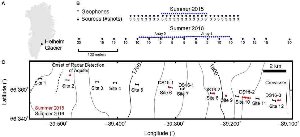
Figure 1. Location of the firn aquifer field site in southeastern Greenland. (A) Geographic context of the field site, Helheim Glacier (black circle). (B) Geometry of seismic deployments; geophones (blue triangles) and source locations (black circle) for summers of 2015 and 2016. Note that in 2016 there were two overlapping arrays (inverted and regular triangles) and the source locations were occupied twice. Values beneath each source indicate the number of shots stacked at the location. (C) Locations of seismic refraction lines; hatches indicate location of first and last geophone in the station geometry shown in (B). Drill sites (DS) from each year are also indicated. Surface topography is obtained from a WorldView-1 (DigitalGlobe©) digital elevation model generated by the Polar Geospatial Center; elevation contour interval is 25 m.

Seismic Refraction Experiment

To assess the structure of the firn aquifer and measure the depth of the aquifer-ice transition, we used a series of active source seismic refraction experiments situated every 1–2 km over a profile 15 km in length (Figure 1C). Each experiment was positioned parallel to the local east-west ice flow line defined by past radar investigations. We used two linear array geometries with geophones spaced every 5 m; (i) a 115 m long array in 2015 (24 stations) and (ii) two 115 m arrays that overlapped at the first station in 2016 (47 unique stations, 1 duplicated location) (Figure 1B). The seismic line was instrumented with Sercel 40 Hz vertical-component geophones. We buried the geophones 5–25 cm into the firn to improve the signal quality and isolate them from noise sources. The burial depth introduced 0.10–0.25 ms of uncertainty into seismic wave travel times, but this uncertainty is similar to or less than the error in picking the P-wave onsets (0.5–1.0 ms) and surface roughness, and is not considered further. In general, the sources of noise at each site were minimal, consisting of blowing wind or snow, distant generator noise, small disturbances in the firn from daily melt, or human movement. Noise conditions were typically better in the morning when the firn was still frozen, and deteriorated in the afternoon as the surface became softer and underwent melt. Seismograms were recorded on a Geometrics Geode multichannel data recorder using a record length of 1 s with a sampling rate of 62.5 μs.

For the active source, we manually struck a 30 × 30 cm, 1.5 cm thick steel plate with a 8-kg sledgehammer, producing seismic waves with a dominant frequency of 150–200 Hz. Where appropriate, multiple hammer strikes (or “shots”) were stacked to enhance the signal-to-noise ratio of waves recorded from the shot location. The initial hammer strike would typically settle the plate into the surface, and subsequent shots would compact the underlying snow by 1–2 cm. Any uncertainties in travel time introduced by the settling of the plate between shots is expected to be minimal, and similar to the uncertainty introduced by the burial of the geophones (0.10–0.25 ms). The attenuation in this environment is quite high (Q = 5–10) so more shots were needed as we moved the source further from the geophone array to produce high signal-to-noise arrivals for analysis.

Two separate source configurations were used in the field experiment. In 2015, sources were spaced regularly with a separation of 10 m and with each consisting of a stack of 3 shots. The number of shots was determined experimentally in the field by determining the minimum number of hammer strikes needed to confidently identify the P-wave onset arriving at the most distant station. The first source was collected 80 m off the line from the first geophone, while the last source was positioned 80 m off the line from the last geophone (Figure 1B). This produced a maximum source-station offset of 195 m in the 2015 array geometry.

In 2016, we modified the source geometry to allow us to sample deeper into the ice sheet, with sources spaced 30 m apart and up to 270 m from the first station in our double array geometry, for a maximum source-station offset of 385 m. Each source location was occupied twice; the line was reshot after repositioning the 24 geophones into the second 115 m array configuration (array 1 and 2 in Figure 1B). The initial source was positioned 270 m from the first geophone, with multiple shots stacked to produce an acceptable signal-to-noise in the recordings. The numbers beneath each source location in Figure 1B indicates the number of shots stacked at each source. The number of shots was determined by experimentation in the field and designed to equalize data quality across different hammer operator abilities and endurance, and to optimize the unfiltered signal-to-noise quality of the seismograms (e.g., Figure 2).

FIGURE 2

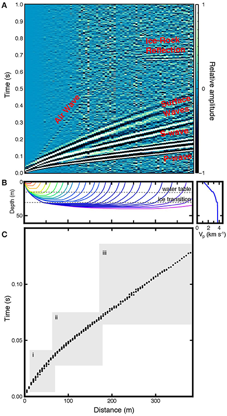
Figure 2. Example active source seismograms, raypaths, and P-wave travel times measured at Site 3 of the study area. (A) Vertical component seismograms with the maximum amplitude of each trace normalized to unity. Interpreted seismic arrivals are labeled in the plot. (B) Theoretical raypaths for P-waves traveling in the hypothetical velocity model on the right. (C) Travel time picks for first arrivals of P-waves at Site 3. The gray regions indicate the distances where P-waves turn and refract: (i) at the water table, (ii) within the firn aquifer and at the ice transition, (iii) within the underlying glacial ice.

The final dataset consisted of operators stacking over 7000 shots, 18 separate seismic lines, and 21,312 individual seismogram recordings from the geophone stations.

Data Processing

Continuous refractions of P-waves are produced by a gradational increase in seismic velocity that bends downward diving waves gradually back upwards toward the surface (e.g., Shearer, 2009). The travel time of the wave is dependent upon the velocities encountered along the raypath of the seismic wave. If any seismic discontinuities are present at depth, a head wave forms along the interface with a travel time slope proportional to the underlying layer seismic velocity. A simple model of a water saturated layer within a gradually increasing firn velocity is shown in Figure 2B, and illustrates how the raypaths of continuous refractions are sensitive to velocity changes in such a medium. Therefore, using travel times of the first arriving P-wave, it is possible to recover the underlying seismic velocities.

Seismograms were visually examined to select the onset travel times of the refracted P-waves arrivals and determine the underlying seismic velocities. Each seismogram was Butterworth band-pass filtered between 40 and 200 Hz. This filtering range was chosen to remove high and low frequency environmental noise and isolate the seismic arrivals. Each P-wave arrival was selected manually according to the first coherent swing deviating from zero amplitude. Consistency between picks was achieved by examining all data for a shot simultaneously and picking on the same polarity across all seismograms (Figure 2). The picking error was defined by pixel accuracy of our picking tool (2–3 pixels), and was less than 0.5 ms.

Inversion for Ice Seismic Velocity Models

To determine the seismic structure of the firn and aquifer, we invert the travel time picks of the continuously refracted waves for one-dimensional (1D) velocity models. Past active source surveys of glacial ice have fit refraction data with an exponential function (e.g., Kirchner and Bentley, 1979). In this study, sharp increases in velocity from the top and bottom of the firn aquifer were anticipated, so we chose to represent the glacier with constant velocity layers in depth (e.g., Shearer, 2009). A further assumption is that the first arriving refracted waves are insensitive to decreases in velocity. In effect, the data could be equally well fit by models with an arbitrary number of low velocity layers. We therefore look for models with velocity increasing with depth. In order to constrain decreasing velocities, other parts of the seismic wavefield—particularly reflected waves and surface waves—could be incorporated in future efforts.

The inversion of first arrivals for layered structure is non-unique in that many velocity models could adequately explain the observations. Instead of inverting for the singular best fitting velocity model, our approach is to instead generate a large number of 1D models that fit the data to within the variance in the travel time picks.

We generate this chain of models using a reversible-jump Markov chain Monte Carlo algorithm (Green, 1995). New models in the chain are proposed by changing the properties of one layer in the current model. In addition to the varying the depth and velocity a layer, we also allow layers to be added or removed (i.e., the transdimensional approach, Bodin and Sambridge, 2009). Proposed changes in velocity and layer depth are randomly drawn from a normal distributions around their current values with standard deviations of 50 m s⁻¹ and 2 m respectively. The depth of proposed new layers is chosen at random, and the velocity drawn at random from between the layers above and below. The velocities are constrained to be between 0 and 4500 m s⁻¹ and the layer depths between 0 and 75 m.

For each proposed new model, the misfit between the observed and modeled travel times is calculated. The model is accepted or rejected based on the change to the misfit and the number of layers (Metropolis et al., 1953). The preferred models explain the data with the fewest number of layers. At regular intervals, the current model is added to an ensemble solution, and in the long term, the frequency with which a model appears in the ensemble is proportional to the probability that it explains the data.

We interpret these the model ensembles to estimate the base of the aquifer and the velocity of the solid ice underlying it. There are two main properties that we can derive from the ensemble of 1D models. First, we find the distribution of possible velocities at each depth (Figure 3A), which allows us to compute a mean velocity and standard deviation. Second, by finding the number of models that place a layer boundary within a certain depth range, we find the probability that there is an increase in velocity at each depth (Figure 3B). From this, we can estimate the confidence intervals on the depths of different interfaces.

FIGURE 3

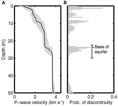
Figure 3. Example model output from Site 11 from the transdimensional reversible-jump Markov chain Monte Carlo inversion. (A) Velocity profile. The mean velocity of models in the ensemble solution is shown as a black line, and the gray region shows the 95% confidence interval. (B) Histogram showing the proportion of models in the ensemble with an increase in velocity at each depth. We interpret this to find the likelihood that a boundary between layers occurs in a given depth range.

Results

Overview of Results

The velocity profiles and discontinuity histograms derived from the inversion are interpreted to estimate aquifer bottom depth (Figure 4). We define the base of the aquifer as the transition from liquid saturated pore space to where the liquid is frozen into ice, which manifests as a transition from increasing to a higher, nearly constant seismic velocity with depth. This definition is derived from ice cores in our study area that showed the base of the aquifer is associated with the onset of clear ice layers resulting from the freezing of aquifer water. We manually select the deepest, most probable discontinuity associated with this boundary (e.g., Figure 3B) and use the surrounding shape of the discontinuity histogram to select the minimum and maximum depths defining the uncertainty in the pick (Table 1). We also derive the local seismic velocity of the ice by selecting the velocity 3–4 m beneath the aquifer layer. As our experimental design was not optimized for imaging the top of the aquifer, we independently obtained depth to the water table from ground penetrating radar reflections that were collected in the field in tandem with the seismic data (Miège et al., 2016). The GPR depths to the water table are estimated from the two-way-travel time of the radar electromagnetic wave between the snow surface and the water-table surface, with a calculated error of ±0.5 m. The aquifer thickness is then the difference between the GPR-derived water table depth and the seismically derived base of the aquifer. A summary of these measurements for each site in our study region is presented in Table 1.

FIGURE 4

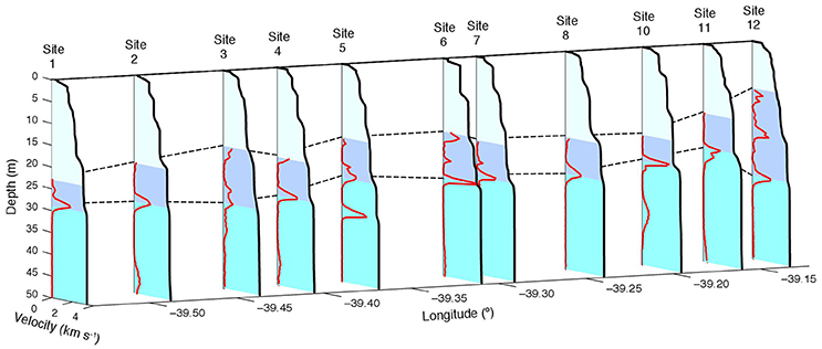
Figure 4. Mean 1D velocity profiles derived from the inversion of travel times measured in the 2016 seismic experiments (solid black lines). The sites locations are as indicated in Figure 1. Light blue is the unsaturated firn, dark blue bands indicate the aquifer layer, and cyan the underlying ice. The water table depth (top dashed line) is derived from radar data, while the aquifer base (lower dashed line) is inferred from the probability of a seismic velocity increase (from 0 to 0.4) associated with the base of the aquifer (Figure 3B).

TABLE 1

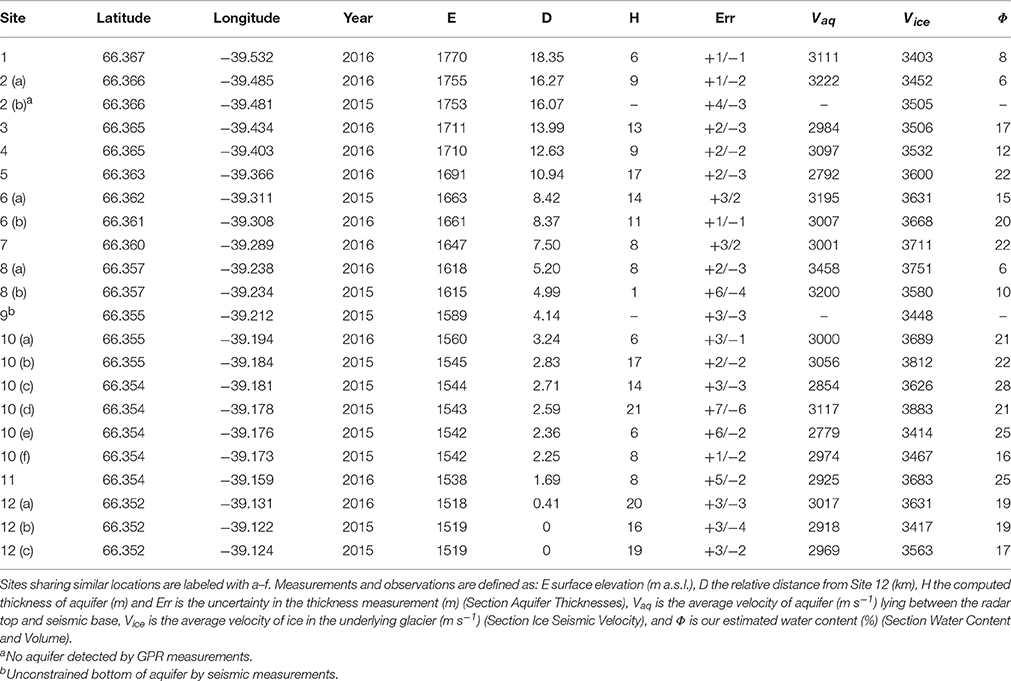
Table 1. Aquifer and ice properties of our seismic survey sites upstream of Helheim glacier.

Aquifer Thicknesses

The depth from both the radar-obtained measurements of the top and seismic-derived measurement of the bottom of the aquifer are summarized in Figure 5. On average, the base of the aquifer lies at 27.7 ± 2.9 m, with an average aquifer thickness of 11.5 ± 5.5 m. While there is temporal and spatial variations in the depth of the water table (Miège et al., 2016), the base of the aquifer appears stable between the 2015 and 2016 field seasons. We note that there is greater uncertainty in the 2015 measurements; this owes to the different array design, as the shorter effective apertures used in 2015 (Figure 1B) had less sensitivity to the base of the aquifer than the 2016 design. This is illustrated for 2015 by the two coincident seismic and GPR depths of the aquifer bottom and top in Figure 5. In this case, the inversion produced results with the largest velocity change near the depth of the water table, but seismic sampling was apparently not deep enough to capture the base, an issue rectified by the larger aperture of the 2016 measurements.

FIGURE 5

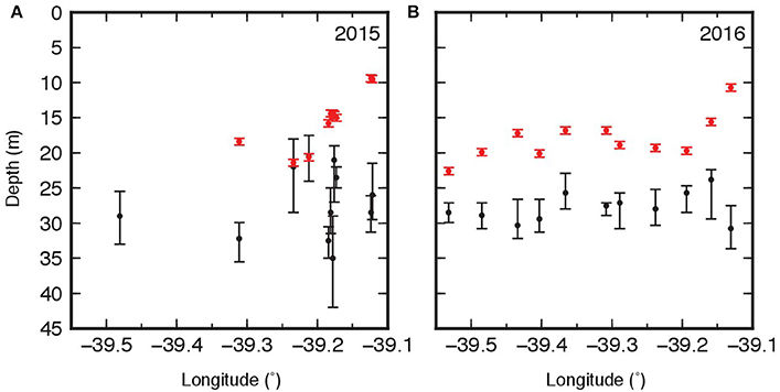
Figure 5. Summary of measurements of the top of aquifer from GPR (red, error ± 50 cm) and seismic determined bottom of aquifer (black; errors from Table 1) along the (A) Summer 2015 and (B) Summer 2016 field sites.

Ice Seismic Velocity

At each site, the seismic velocity of the glacial ice and its standard deviation were derived from the 1D inversion at a depth 3–4 m below the inferred base of the aquifer (Figure 6). We find significant variation between the ice velocities as a function of location along the profile (Figure 1B). On average, the ice in our study region has a velocity of 3590 ± 133 m s⁻¹, however we note that in 2015 we observed more variability in ice seismic velocities (3400–3900 m s⁻¹) than in 2016 (3700–3800 m s⁻¹) for the downslope regions. We attribute this difference to the larger array aperture in 2016 that provided improved sensitivity to the deeper ice structure compared to the 2015 array. We calculate that the deepest continuously refracted waves for the 2015 array reached a depth of 30–35 m, while the continuously refracted wave in the 2016 survey reached a depth of 50–55 m. We also observed a systematic increase in ice velocity moving downslope to Site 9; this may represent the addition of ice lenses, compaction processes, increased ice flow or frozen aquifers (Harper et al., 2012). We explore this further in the discussion.

FIGURE 6

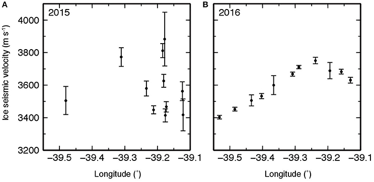
Figure 6. Velocity of the ice underlying the firn aquifer, as measured in the summer of (A) 2015 and (B) 2016. Error bars are derived from the 1D inversion (Figure 3B).

Water Content and Volume

Seismic velocities are sensitive to the relative fraction of liquid and solid in a two-phase interconnected mixture (Biot, 1956; Hajra and Mukhopadhyay, 1982). We can relate these two quantities using (Equation 1) (Wyllie et al., 1956), which describes the contribution of water content (ϕ) to the P-wave velocity (v_aq) observed in the aquifer layer of each seismic site.

$\varphi =\frac{v_{H_{2}O}\left(\raisebox{1ex}{$v_{ice}$}\!\left/ \!\raisebox{-1ex}{$v_{aq}$}\right.-1\right)}{\left(v_{ice}-v_{H_{2}O}\right)}\times 100\%(1)$

The value of ϕ is proportional to the relative seismic velocity of the water in the saturated pore space, (v_H2O = 1450 m s⁻¹; Shearer, 2009), the seismic velocity of ice (v_ice) that we derive from our inversion results (Table 1), and the average seismic velocity of the aquifer V_aq, also in Table 1. Our porosity estimate from this method is an upper bound as we exclude the effects of air bubbles trapped within the saturated pore space (~6% on average, Koenig et al., 2014), which would further reduce seismic velocity.

We observe spatial and temporal changes in water content within the aquifer (Figure 7). We omit locations where we could not determine the aquifer base or water table, and sampling of the aquifer at higher altitudes further to the west was limited to one site in 2015 (Site 2b). At this location, no reflection in the GPR data corresponding to the water table was identified, so we interpret this region as having minimal water content in 2015. In 2016, Site 1 was dry, while Site 2a situated near Site 2b indicated the presence of water in both the seismic and radar investigations (Figure 7). These observations confirm that the aquifer is expanding inland to the west and at higher elevations, which is in agreement with airborne radar and remote sensing observations (Jeffries et al., 2015; Miège et al., 2016). In both years, we calculate that the average water content of the aquifer saturated zone ranges from 8 to 24%.

FIGURE 7

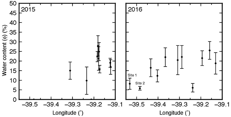
Figure 7. Seismic velocity-derived water content (Φ) of the saturated pore space within the firn aquifer for years 2015 and 2016. Error bars are derived from the uncertainty in the thickness measurements.

We then use aquifer water content to calculate firn storage capacity M_H2O (in kg m⁻²) for each site by estimating the total mass of water stored per 1 m² of aquifer:

$\begin{array}{rc}{M}_{H_{2}O}=\varphi H\rho .& (2)\end{array}$

where H is aquifer thickness (m), ϕ is the water content (%), and ρ is the density of water (1000 kg m⁻³). Figure 8 shows the result of this calculation for firn water storage capacity at each site. We calculate that the aquifer in our study region has an average storage capacity of 2070 ± 1360 kg m⁻². There is a general increase in water storage capacity within the aquifer, moving from a minimum at the highest elevations to the west, and increasing downslope to the east.

FIGURE 8

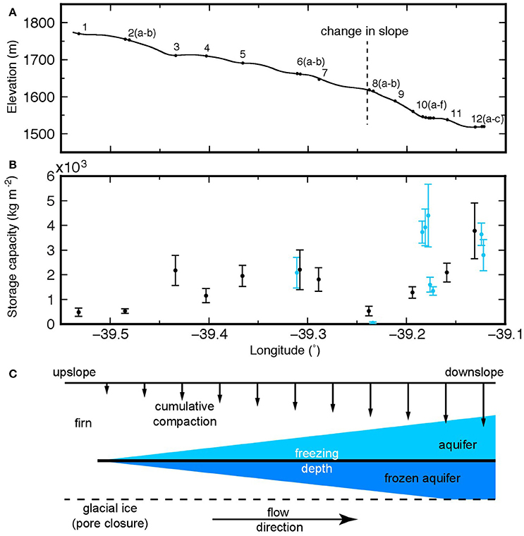
Figure 8. Aquifer water storage capacity across our study region. (A) Elevation profile along flow line and location of the major change in slope across our study region. Surface topography is obtained from a WorldView-1 (DigitalGlobe©) digital elevation model generated by the Polar Geospatial Center. (B) 2015 measurements shown in cyan, 2016 measurements shown in black. Error bars are determined from the uncertainty in the water content measurements. (C) Inferred structure of the Greenland ice sheet aquifer.

Discussion

Effective media estimations require knowledge of the matrix and fluid velocities to determine the bulk velocity of a fluid-filled medium (e.g., Biot, 1956; Wyllie et al., 1956). Here we assign a value of 1450 m s⁻¹ for liquid water and 343 m s⁻¹ for air (Shearer, 2009). An assembled dataset of laboratory and in situ measurements of firn and ice velocity presented in Kohnen (1974) show that polycrystalline ice at 0°C should have a seismic velocity of 3795 m s⁻¹. This is comparable, given the uncertainties, to the highest velocities observed in our study region in 2015, 3883 ± 165 m s⁻¹ at site 10 days; in 2016, 3751 ± 20 m s⁻¹ at site 8a. However, the majority of sites across our study region are systematically slower than this expected value for ice, up to 10% less at Site 1. In the 2015 active source experiments, this discrepancy can be attributed to the 195 m effective array aperture and incomplete sampling of the region beneath the aquifer. The continuously refracted seismic waves in these experiments refracted very near the base of the aquifer (25–30 m) and may not have sampled deep enough to resolve ice velocity. This is supported by the comparably higher errors derived from the inversions of the ice seismic velocity in 2015 vs. 2016 (Figure 6). In the 2016 experiments, there is a systematic increase in seismic velocity derived from Site 1 (3403 ± 11 m s⁻¹) eastward and downslope to Site 8a (3751 ± 20 m s⁻¹), and then a small decrease moving eastward and downslope to Site 12a (3631 ± 18 m s⁻¹). For these experiments the effective array aperture is 385 m, with the deepest diving rays sampling near 50–55 m depth, well below the base of the aquifer. Given this deeper sampling, we interpret the pattern of ice velocities in 2016 as a well-resolved feature of the study region. Furthermore, since these ice velocities are up to 10% less than that of polycrystalline ice, we suggest that the base of the firn aquifer in these locations cannot correspond to the pore closure depth within the firn, and is associated with a different mechanism.

In situ measurements of firn and ice velocity from Kohnen and Bentley (1973) show that dry firn velocities increase exponentially with depth and are related to the mechanisms driving compaction within the firn. Densification in the upper 11–14 m of firn is driven by mechanical rearrangement of grain boundaries, and then switches to recrystallization of grains down to 56–64 m depth. Below these depths, any further densification results from the compression of air bubbles in the ice. Liquid water percolating into and through the firn would descend to a depth where it either reaches an impermeable boundary (e.g., pore closure at the firn-ice transition) or falls below 0°C and freezes into the pore space. The freezing depth in our study region occurs near 30–35 m depth (Koenig et al., 2014) and is shallower than the expected depth of pore closure (56–64 m) reported by Kohnen and Bentley (1973). The base of the aquifer in our study (27.7 ± 2.9 m) is therefore closer to the freezing depth than the pore closure depth, so we infer that the seismic velocity jump at the base of the aquifer corresponds to freezing of liquid water into the pore space. Since the firn at this depth has not completely recrystallized into ice, the effective velocity is dependent upon the amount of frozen water added at the base of the aquifer. We also observe multiple 0.2–0.5 m layers of clear ice in cores drilled in the summers of 2015 and 2016 down to depths of 55 m (Koenig et al., 2014). The clear ice layers are more abundant in cores drilled further eastward and downslope (Figure 1C). Clear ice forms by freezing of a layer of older aquifer water; addition of material to the ice sheet will compact and drive the aquifer layer below the freezing isotherm. It is expected that regions with older aquifer would therefore be underlain by a series of frozen clear ice layers. Subsequent addition of these layers each year would increase seismic velocity as the number of frozen-in clear ice layers increases with the velocity of the ice beneath the aquifer and is expected to increase as the ice moves the aquifer to lower elevation (Figure 8).

Our estimate of water content in the aquifer is dependent upon several assumptions about the relationship between seismic velocity, porosity, and fluid content. First, we use the velocity of the ice directly below the aquifer layer rather than the expected velocity of polycrystalline ice at 0°C (3795 m s⁻¹). The Wyllie average assumes prior knowledge about the velocity of the fluid and matrix; using the velocity of polycrystalline ice would overestimate water content as it assumes the unsaturated firn matrix would behave as fully recrystallized ice (Kohnen and Bentley, 1973). The firn is still undergoing compaction and thus will have a lower effective velocity than pure ice. We therefore choose to use the velocity of the ice directly beneath the aquifer to derive a porosity estimate to minimize any offset expected from the incomplete compaction of the firn matrix. Second, we use the average of the velocity across the aquifer layer to compare to the underlying ice. This is obtained by finding the mean velocity lying between the GPR-defined top of the aquifer, and seismically defined base. This does not take into account vertical variations of water content that could be present within the aquifer. Integrating the porosity across the layer would provide a more appropriate estimate; however the resolution of our inversion typically places a singular layer at aquifer range of depths, so any attempt to refine the stratification in the aquifer layer would be better served by allowing the inversion to fit gradients rather than layers. This will be incorporated into future work. Third, we neglect the effect of air bubbles on the seismic velocity, making our estimate of porosity an upper bound on the water content within the aquifer layer. The addition of air bubbles will reduce the amount of water required to explain the inversion-derived seismic velocity within the aquifer layer. For example, adding 6% air to the pore space in the aquifer at site 12a will reduce the derived porosity from 18.8 to 10.5% and our storage capacity down from 3780 to 1946 kg m⁻². Since we do not have a way to independently evaluate air content within the aquifer layer, we choose to report the upper bound estimate of water content assuming no contribution from the air.

Past estimates of water content in the aquifer obtained by Koenig et al. (2014) via ice cores found a firn capacity (in kg m⁻²) of 2150 kg m⁻² assuming a 14-m thick aquifer with an aerial extent of 70 ± 10 × 10³ km² or 980 ± 140 km³. Using radar mapping of the lateral extent of the firn aquifer, they estimated the total mass of Greenland aquifer to contain 140 ± 20 gigatons (Gt) of liquid water. With our seismic methodology, we are able to examine the lateral variability in aquifer thickness and water content along an elevation 2-D transect and refine this volume estimate (Figure 8). With these improved estimates of aquifer thickness (11.5 ± 5.5 m) and seismically-derived water content (8–24%), we find that water volume ranges from 0 to 4400 kg m⁻²; with an average value of 2070 ± 1360 kg m⁻², similar to the Koenig et al. (2014) value. Furthermore, in 2016, the spatial extent of the Helheim Glacier aquifer is estimated at 2286 km² (Miège et al., 2016). With these values, we estimate that the total volume of water in the Helheim aquifer is 4.7 ± 3.1 Gt, similar to the ice core estimates of Koenig et al. (2014).

The values reported above represent bulk averages; we also detect spatial variability in the water content of the aquifer layer. This value evolves from 530 kg m⁻² at Site 2 up to 3800 kg m⁻² at Site 12 (Figure 8). Site 12 is 250 m lower in elevation than Site 2, with undulations in the surface topography (and underlying water table) with wavelengths of 1–2 km. The increase in water content generally mirrors the topography and is expected to increase due to more melt percolating into the system at lower and presumably warmer elevations. The water table approaches the surface (10.7 m) at Site 12 (Figure 5) where we seismically estimate the highest water storage capacities for the aquifer. There is also a large decrease in water content near Sites 8 and 9 (530 and 50 kg m⁻², respectively) where there is a noticeable change in surface slope (marked in Figure 8). Cores drilled at Site 8a in 2016 revealed a very thin (<1 m) aquifer at this location. The lack of water at this location could reflect a 3-dimensional change in the aquifer, including increased flow rates at the higher slope, drainage into a buried crevasse, diversion around a local geographic feature, or a locally shallow firn-ice transition and lack of permeability within the ice. We cannot distinguish between these possibilities without further investigation of this feature in the field.

At most sites with seismic measurements in both years (e.g., Sites 6, 8, 12), there is agreement between the estimated water storage capacities. However, at Site 10, we observed a discrepancy in the estimated storage capacities from 2015 to 2016 (Figure 8). Sites 9 and 10 were our noisiest sites, with both data collected during active drill site and team operations in 2015 (individuals walking, generators, etc.). In the resulting inversions, we were unable to uniquely derive aquifer properties at Site 9 owing to coincidence of the radar selected water table and seismological discontinuities. This discrepancy was also observed in the seismic velocity measurements of the ice; in general the sites expressed much lower ice seismic velocity than their 2016 counterparts (Figure 6). These uncertainties were not identified until after the 2015 field season, to which we responded by the expansion of the effective array aperture length of the seismic array from 195 m to 385 m. To offset any potential site noise, we also increased the number of stacked shots in 2015 (3 shots) to >5 in 2016 (Figure 1B). These measures improved the overall quality of the deepest diving seismic waves that sample the base of the aquifer. The combined effects of higher signal-to-noise and deeper sampling thus make us more confident in the 2016 results.

To summarize, in 2015 and 2016, we used refraction seismology to temporally and spatially sample the structure of a firn aquifer on the southeastern GrIS, and determined that the base of this aquifer lies on average 27.7 ± 2.9 m beneath the surface, with an average thickness of 11.5 ± 5.5 m. We relate the change in seismic wave speed across the aquifer to pore saturation of water, finding the aquifer has an average pore space of 16 ± 8%, with considerable variation in storage capacity of water along the studied east-west regional flow line. We also find that the seismic base of the aquifer corresponds to the freezing point of liquid water within the pore space. Subsequent addition of these frozen layers beneath the aquifer from year-to-year produces a high velocity seismic layer directly beneath the aquifer. From 2015 to 2016, we observed a 1–2 km uphill expansion of the aquifer system, with a dry site seismically investigated in 2015 now having a 530 kg m⁻² water content in 2016 (Site 2). We estimate that the volume of water stored in the aquifer across the entire region upstream of Helheim glacier to be 4.7 ± 3.1 gigatons, a value comparable to prior estimates by Koenig et al. (2014) from ice core sampling of the aquifer. Using seismics, we reveal the relationship between the percolation of meltwater through the aquifer system, the addition of frozen surface melt at depth beneath the aquifer layer, and ultimately constrain the impact of ice sheet aquifers on sea level rise.

Author Contributions

The manuscript was written by LM and NS and edited by all the authors. Data analysis was performed by LM and NS; and SB wrote the THB inversion. CM provided the radar depth of the aquifer and estimates of aquifer extent. Seismic data were collected by LM, NS, RF, CM, SL, OM, AL, and DS. All authors agree to be accountable for the content of this work.

Funding

Support for this research was provided by the National Science Foundation; LM and NS were supported by PLR-1417993. SB was supported by EAR-1349771; and DS, RF, OM, and CM were supported by PLR-1417987. LK was supported by NASA Cryospheric Sciences program NASA Award NNX15AC62G. SL was supported by an NWO ALW Veni grant number 865.15.023.

Conflict of Interest Statement

The authors declare that the research was conducted in the absence of any commercial or financial relationships that could be construed as a potential conflict of interest.

Acknowledgments

We thank Kyli Cosper and the entire CH2MHILL PFS Team for excellent field logistics and support. We thank our two review editors for providing thorough and insight commentary that helped to greatly improve the quality of the manuscript. Seismic instruments were provided by the Incorporated Research Institutions for Seismology (IRIS) through the PASSCAL Instrument Center at New Mexico Tech. Seismic data collected will be made available through the IRIS Data Management Center as an assembled data set. GPR data will be made available through the Arctic Data Center. The facilities of the IRIS Consortium are supported by the National Science Foundation under Cooperative Agreement EAR-1261681 and the DOE National Nuclear Security Administration. Figures in this manuscript were constructed using the Generic Mapping Toolkit (Wessel et al., 2013).

References

Albert, D. (1998). Theoretical modeling of seismic noise propagation in firn at the south pole, Antarctica. Geophys. Res. Lett. 25, 4257–4260. doi: 10.1029/1998gl900155

CrossRef Full Text | Google Scholar

Biot, M. A. (1956). The theory of propagation of elastic waves in a fluid-saturated porous solid. I. Low frequency range. II. Higher frequency range. J. Acoust. Soc. Am. 28, 168–178, 179–191. doi: 10.1121/1.1908239

CrossRef Full Text | Google Scholar

Blankenship, D. D., Bentley, C. R., Rooney, S. T., and Alley, R. B. (1986). Seismic measurements reveal a saturated porous layer beneath an active Antarctic ice stream. Nature 322, 54–57. doi: 10.1038/322054a0

CrossRef Full Text | Google Scholar

Bodin, T., and Sambridge, M. (2009). Seismic tomography with the reversible jump algorithm. Geophys. J. Int. 178, 1411–1436. doi: 10.1111/j.1365-246X.2009.04226.x

CrossRef Full Text | Google Scholar

Christianson, K., Kohler, J., Alley, R. B., Nuth, C., and Pelt, W. J. J. (2015). Dynamic perennial firn aquifer on an Arctic glacier. Geophys. Res. Lett. 42, 1418–1426. doi: 10.1002/2014GL062806

CrossRef Full Text | Google Scholar

Enderlin, E. M., Howat, I. M., Jeong, S., Noh, M. J., van Angelen, J. H., and van den Broeke, M. R. (2014). An improved mass budget for the Greenland ice sheet. Geophys. Res. Lett. 41, 866–872. doi: 10.1002/2013GL059010

CrossRef Full Text | Google Scholar

Ettema, J., van den Broeke, M. R., van Meijgaard, E., van de Berg, W. J., Bamber, J. L., Box, J. E., et al. (2009). Higher surface mass balance of the Greenland ice sheet revealed by high-resolution climate modeling. Geophys. Res. Lett. 36:L12501. doi: 10.1029/2009GL038110

CrossRef Full Text | Google Scholar

Fettweis, X., Franco, B., Tedesco, M., van Angelen, J. H., Lenaerts, J. T. M., van den Broeke, M. R., et al. (2013). Estimating the Greenland ice sheet surface mass balance contribution to future sea level rise using the regional atmospheric climate model MAR. Cryosphere 7, 469–489. doi: 10.5194/tc-7-469-2013

CrossRef Full Text | Google Scholar

Forster, R. R., Box, J. E., van den Broeke, M. R., Miège, C., Burgess, E. W., van Angelen, J. H., et al. (2014). Extensive liquid meltwater storage in firn within the Greenland ice sheet. Nat. Geosci. 7, 95–98. doi: 10.1038/ngeo2043

CrossRef Full Text | Google Scholar

Gogineni, S. P. (2012). CReSIS RDSData with Digital Data. Lawrence. Available online at: http://data.cresis.ku.edu/

Green, P. J. (1995). Reversible jump Markov chain Monte Carlo computation and Bayesian model determination. Biometrika 82, 711–732. doi: 10.1093/biomet/82.4.711

CrossRef Full Text | Google Scholar

Hajra, S., and Mukhopadhyay, A. (1982). Reflection and refraction of seismic waves incident obliquely at the boundary of a liquid-saturated porous solid. Bull. Seismol. Soc. Am. 72, 1509–1533.

Google Scholar

Harper, J., Humphrey, N., Pfeffer, W. T., Brown, J., and Fettweis, X. (2012). Greenland ice-sheet contribution to sea-level rise buffered by meltwater storage in firn. Nature 491, 240–243. doi: 10.1038/nature11566

PubMed Abstract | CrossRef Full Text | Google Scholar

Horgan, H. J., Anandakrishnan, S., Jacobel, R. W., Christianson, K., Alley, R. B., Heeszel, D. S., et al. (2012). Subglacial Lake Whillans—Seismic observations of a shallow active reservoir beneath a West Antarctic ice stream. Earth Planet. Sci. Lett. 331–332, 201–209. doi: 10.1016/j.epsl.2012.02.023

CrossRef Full Text | Google Scholar

Humphrey, N. F., Harper, J. T., and Pfeffer, W. T. (2012). Thermal tracking of meltwater retention in Greenland's accumulation area. J. Geophys. Res. 117:F01010. doi: 10.1029/2011JF002083

CrossRef Full Text | Google Scholar

Jarvis, E. P., and King, E. C. (1995). Seismic investigation of the Larsen Ice Shelf, Antarctica: in search of the Larsen Basin. Antarct. Sci. 7, 181–190. doi: 10.1017/S0954102095000241

CrossRef Full Text | Google Scholar

Jeffries, M. O., Richter-Menge, J., and Overland, J. E. (Eds.). (2015). Arctic Report Card 2015. Available online at: http://www.arctic.noaa.gov/Report-Card

Johnson, M. R., and Smith, A. M. (1997). Seabed topography under the southern and western Ronne Ice Shelf, derived from seismic surveys. Antarct. Sci. 9, 201–208. doi: 10.1017/S0954102097000254

CrossRef Full Text | Google Scholar

Kirchner, J. F., and Bentley, C. R. (1979). Seismic short-refraction studies on the Ross Ice Shelf, Antarctica. J. Glaciol. 24, 313–319.

Google Scholar

Koenig, L. S., Miège, C., Forster, R. R., and Brucker, L. (2014). Initial in situ measurements of perennial meltwater storage in the Greenland firn aquifer. Geophys. Res. Lett. 41, 81–85. doi: 10.1002/2013GL058083

CrossRef Full Text | Google Scholar

Kohnen, H. (1974). Temperature dependence of seismic waves in ice. J. Glaciol. 13, 144–147.

Google Scholar

Kohnen, H., and Bentley, C. (1973). Seismic refraction and reflection measurements at “byrd” station, Antarctica. J. Glaciol. 12, 101–111.

Google Scholar

McMahon, K. L., and Lackie, M. A. (2006). Seismic reflection studies of the Amery Ice Shelf, East Antarctica: delineating meteoric and marine ice. Geophys. J. Int. 166, 757–766. doi: 10.1111/j.1365-246X.2006.03043.x

CrossRef Full Text | Google Scholar

Metropolis, N., Rosenbluth, A. W., Rosenbluth, M. N., Teller, A. H., and Teller, E. (1953). Equation of state calculations by fast computing machines. J. Chem. Phys. 21, 1087–1092. doi: 10.1063/1.1699114

CrossRef Full Text | Google Scholar

Miège, C., Forster, R. R., Brucker, L., Koenig, L. S., Solomon, D. K., Paden, J. D., et al. (2016). Spatial extent and temporal variability of Greenland firn aquifers detected by ground and airborne radars, J. Geophys. Res. Earth Surf. 121, 2381–2398. doi: 10.1002/2016JF003869

CrossRef Full Text

Munneke, P. K., Ligtenberg, S. R. M., van den Broeke, M. R., van Angelen, J. H., and Forster, R. R. (2014). Explaining the presence of perennial liquid water bodies in the firn of the Greenland Ice Sheet. Geophys. Res. Lett. 41, 476–483. doi: 10.1002/2013GL058389

CrossRef Full Text | Google Scholar

Neff, P. D., Steig, E. J., Clark, D. H., McConnell, J. R., Pettit, E. C., and Menounos, B. (2012). Ice-core net snow accumulation and seasonal snow chemistry at a temperate-glacier site: Mount Waddington, southwest British Columbia, Canada. J. Glaciol. 58, 1165–1175. doi: 10.3189/2012JoG12J078

CrossRef Full Text | Google Scholar

Rennermalm, A. K., Moustafa, S. E. Mioduszewski, J., Chu, V. W., Forster, R. R., Hagedorn, B., et al. (2013). Understanding Greenland ice sheet hydrology using an integrated multi-scale approach. Environ. Res. Lett. 8:015017. doi: 10.7916/D88K7916

CrossRef Full Text | Google Scholar

Rignot, E., Velicogna, I., van den Broeke, M. R., Monaghan, A., and Lenaerts, J. T. (2011). Acceleration of the contribution of the Greenland and Antarctic ice sheets to sea level rise. Geophys. Res. Lett. 38:L05503. doi: 10.1029/2011GL046583

CrossRef Full Text | Google Scholar

Shearer, P. M. (2009). Introduction to Seismology. Cambridge: Cambridge University Press.

Google Scholar

Smith, A. M., Jordan, T. A., Ferraccioli, F., and Bingham, R. G. (2013). Influence of subglacial conditions on ice stream dynamics: seismic and potential field data from Pine Island Glacier, West Antarctica. J. Geophys. Res. Solid Earth 118, 1471–1482. doi: 10.1029/2012JB009582

CrossRef Full Text | Google Scholar

van Angelen, J. H., Lenaerts, J. T. M., van den Broeke, M. R., Fettweis, X., and van Meijgaard, E. (2013). Rapid loss of firn pore space accelerates 21st century Greenland mass loss. Geophys. Res. Lett. 40, 2109–2113. doi: 10.1002/grl.50490

CrossRef Full Text | Google Scholar

van den Broeke, M., Bamber, J., Ettema, J., Rignot, E., Schrama, E., van de Berg, W. J., et al. (2009). Partitioning recent greenland mass loss. Science 326, 984–986. doi: 10.1126/science.1178176

PubMed Abstract | CrossRef Full Text | Google Scholar

Vernon, C. L., Bamber, J. L., Box, J. E., van den Broeke, M. R., Fettweis, X., Hanna, E., et al. (2013). Surface mass balance model intercomparison for the Greenland ice sheet. Cryosphere 7, 599–614. doi: 10.5194/tc-7-599-2013

CrossRef Full Text | Google Scholar

Wessel, P., Smith, W. H. F., Scharroo, R., Luis, J. F., and Wobbe, F. (2013). Generic Mapping Tools: improved version released, EOS Trans. AGU 94, 409–410. doi: 10.1002/2013EO450001

CrossRef Full Text | Google Scholar

Winberry, J. P., Anandakrishnan, S., and Alley, R. B. (2009). Seismic observations of transient subglacial water-flow beneath MacAyeal Ice Stream, West Antarctica. Geophys. Res. Lett. 36:L11502. doi: 10.1029/2009GL037730

CrossRef Full Text | Google Scholar

Wyllie, M. R. J., Gregory, A. R., and Gardner, L. W. (1956). Elastic wave velocities in heterogeneous and porous media. Geophysics 21, 41–70. doi: 10.1190/1.1438217

CrossRef Full Text | Google Scholar